Chapter 10. Electricity and Magnetism
Hall sensors detect a magnetic field. They come in different varieties: some just detect the presence of a magnet, while others can tell you the strength of the magnetic field in teslas.
Voltage and current sensors work like a multimeter, measuring electricity passing through them. They can easily measure power that would otherwise break a microcontroller’s analog input pin.
An electronic compass can tell you where magnetic north is. Better ones combine an accelerometer, so that they can point to north even when tilted.
The sun’s north and south poles change places about every 11 years. As of this writing, we’re waiting for the flip to happen at any week now. However, you don’t have to worry about the Earth’s poles flipping on you. The last time that happened was 780,000 years ago.
Experiment: Voltage and Current
In this experiment, you’ll use the AttoPilot to measure voltage of a battery pack.
Are the batteries running out, and how much power is your robot’s motor draining? AttoPilot Compact DC Voltage and Current Sense measures voltage and current. It measures big voltage and current, and then reports it with analog output.
AttoPilot can measure a lot of power. The most powerful model is rated for 50 V and 180 A. Power (P) is a function of voltage (U) and current (I):
P = UI = 50 V * 180 A = 9000 VA = 9000 W = 9 kW
You are likely to also see this expressed with watts (W) as a function of voltage (V) and current (A):
W = VA = 50 V * 180 A = 9000 W = 9 kW
The 50 V/ 180 A model of the AttoPilot sensor can handle 9 kilowatts. You can’t. Stay safe and use only sensible voltages, like batteries and USB power.
| Model | Voltage U, output/measured | Current I, output/measured | Comment |
13.6 V / 45 A | 242.3 mV / V | 73.20 mV / A | Used in this experiment |
50 V / 90 A | 63.69 mV / V | 36.60 mV / A | |
50 V / 180 A | 63.69 mV / V | 18.30 mV / A | 9 kW |
Because such power can’t be safely handled in most projects, we used the 13 V / 45 A model for this test.
P = UI = 13 V * 45 A = 585 W # model used here
The AttoPilot has two analog outputs. One reports current; the other reports voltage. The maximum output is 3.3 V—considerably less than the maximum 50 V measured. The conversion factors for the 13.6 V / 45 A model used here are calculated from the component’s maximum specs. Using 13.6 V / 45 A model as an example, here’s the formula for current:
3.3 V output / 45 A measured = 73.3 mV output / A measured
But in your code, you’ll switch things around:
45 A measured/ 3.3 V output = 13.6363 A measured / V output
So when you want to calculate the measured current, you can multiply the voltage you read from the current sense output by 13.6363:
0.05 V output * 13.6363 ≈ .6818 A = 681.8 mA
And here’s the formula for voltage:
3.3 V output / 13.6 V measured = 242.6 mV output / V measured
To express this in a way that’s useful for calculating measured voltage in your code, look at it this way:
13.6 V measured / 3.3 V output = 4.1212 V measured / V output
When you want to calculate the measured voltage, you can multiply the voltage you read on the voltage sense output by 4.1212:
1.213 V output * 4.1212 ≈ 5 V
AttoPilot Code and Connection for Arduino
Figure 10-1 shows the connections for Arduino. Wire it up as shown, and then run the sketch shown in Example 10-1.

// attopilot_voltage.ino - measure current and voltage with Attopilot 13.6V/45A// (c) BotBook.com - Karvinen, Karvinen, ValtokariintcurrentPin=A0;intvoltagePin=A1;voidsetup(){Serial.begin(115200);pinMode(currentPin,INPUT);pinMode(voltagePin,INPUT);}floatcurrent(){floatraw=analogRead(currentPin);Serial.println(raw);floatpercent=raw/1023.0;//floatvolts=percent*5.0;//floatsensedCurrent=volts*45/3.3;// A/V //returnsensedCurrent;// A //}floatvoltage(){floatraw=analogRead(voltagePin);floatpercent=raw/1023.0;floatvolts=percent*5.0;floatsensedVolts=volts*13.6/3.3;// V/V //returnsensedVolts;// V}voidloop(){Serial.("Current:");Serial.(current(),4);Serial.println("A");Serial.("Voltage:");Serial.(voltage());Serial.println("V");delay(200);// ms}

The maximum reading of
analogRead()is 1023, so we calculate the reading as a percentage of that maximum.
Five volts is the maximum voltage of Arduino’s
analogRead(). Five volts corresponds to a raw value of 1023.
The conversion factor is 45 A measured / 3.3 V output ≈ 13.7 A/V. See also Table 10-1.

Return current in amperes. It’s always a good idea to include the unit in your comments.

The voltage conversion factor is
V measured max / V output max.
AttoPilot Code and Connection for Raspberry Pi
Figure 10-2 shows the connections for the Raspberry Pi and AttoPilot. Hook everything up as shown, and then run the program in Example 10-2.

# attopilot_voltage.py - measure current and voltage with Attopilot 13.6V/45A# (c) BotBook.com - Karvinen, Karvinen, Valtokariimporttimeimportbotbook_mcp3002asmcp#defreadVoltage():raw=mcp.readAnalog(0,1)#percent=raw/1023.0#volts=percent*3.3#sensedVolts=volts*13.6/3.3# V/V #returnsensedVolts# VdefreadCurrent():raw=mcp.readAnalog(0,0)percent=raw/1023.0volts=percent*3.3sensedCurrent=volts*45.0/3.3# A/V #returnsensedCurrent# Adefmain():whileTrue:voltage=readVoltage()current=readCurrent()("Current%.2fA"%current)("Voltage%.2fV"%voltage)time.sleep(0.5)# sif__name__=="__main__":main()
-
Import the library for the MCP3002 analog-to-digital converter chip. The library botbook_mcp3002.py must be in the same directory as this program (attopilot_voltage.py).
-
Read the second channel. The AttoPilot voltage and current sensing outputs are connected to different channels.
-
1023 is the maximum value of
readAnalog(). It corresponds to 3.3 V.-
The maximum GPIO voltage for the Raspberry Pi 3.3 V.
-
Conversion factors are calculated just like with Arduino. The voltage conversion factor is
V measured max / V output max.
The conversion factor is 45 A measured / 3.3 V output ≈ 13.7 A/V. See also Table 10-1.
Experiment: Is It Magnetic?
A Hall effect sensor measures a magnetic field. Hall effect sensors are used in bike speedometers, where a magnet on the wheel helps the sensor count revolutions.
A magnetic field causes electrons to divert from their straight path, causing a voltage change in a conductor. This is the Hall effect.
The sensor reports a magnetic field as a voltage. This voltage can be read just like an analog resistance sensor, using analogRead() or botbook_mcp3002.readAnalog().
This effect is implemented in sensors from a variety of manufacturers. We used the KY-024 Magnetic Detecting Sensor Module (part number 232563) from http://dx.com, shown in Figure 10-3.

Hall Effect Sensor Code and Connection for Arduino
Figure 10-4 shows the connections for Arduino. Wire it up as shown, and then run the sketch shown in Example 10-3.
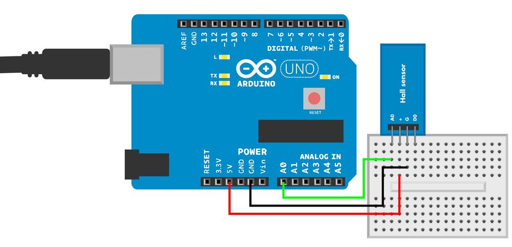
// hall_sensor.ino - print raw value and magnets pole// (c) BotBook.com - Karvinen, Karvinen, ValtokariconstinthallPin=A0;intrawMagneticStrength=-1;//intzeroLevel=527;//voidsetup(){Serial.begin(115200);pinMode(hallPin,INPUT);}voidloop(){rawMagneticStrength=analogRead(hallPin);//Serial.("Raw strength:");Serial.println(rawMagneticStrength);intzeroedStrength=rawMagneticStrength-zeroLevel;// If you know your Hall sensor's conversion from// voltage to gauss then you can do it here// zeroedStrength * conversionSerial.("Zeroed strength:");Serial.println(zeroedStrength);if(zeroedStrength>0){Serial.println("South pole");}elseif(zeroedStrength<0){Serial.println("North pole");}delay(600);// ms}
-
Initialize to a value that wouldn’t come up as a result from reading the sensor. That way, you know that if you see this value in your running code, there’s a problem you need to debug.
-
This is the raw
analogRead()value when there is no magnetic field. Our sensor reports 527 when there is no magnetic field. The manufacturer’s specification gives 500 (raw), presumably for 5 V logic level. If you see different values in the Arduino Serial Monitor when you have no magnetic field, you may need to adjust thezeroLevelvariable.-
The Hall sensor works just like an analog resistance sensor, even though it’s not a resistor.
Hall Effect Sensor Code and Connection for Raspberry Pi
Figure 10-5 shows the connections for Raspberry Pi. Hook them up as shown, and then run the code shown in Example 10-4.

# hall_sensor.py - print raw value and magnets pole# (c) BotBook.com - Karvinen, Karvinen, Valtokariimporttimeimportbotbook_mcp3002asmcp#zeroLevel=388#defmain():whileTrue:rawMagneticStrength=mcp.readAnalog()("Raw strength:%i"%rawMagneticStrength)zeroedStrength=rawMagneticStrength-zeroLevel("Zeroed strength:%i"%zeroedStrength)if(zeroedStrength>0):("South pole")elif(zeroedStrength<0):("North pole")time.sleep(0.5)if__name__=="__main__":main()
-
The library (botbook_mcp3002.py) must be in the same directory as this program. You must also install the spidev library, which is imported by botbook_mcp3002. See the comments in the beginning of botbook_mcp3002/botbook_mcp3002.py or Installing SpiDev.
-
zeroLevelis the raw output ofreadAnalog()when no magnetic field affects the sensor. Our test gave us 388 for our sensor. The manufacturer’s specifications give a raw value of 500 under a 5 V logic level, which would give a raw value of 330 forzeroLevelat 3.3 V:500 * (3.3/5) = 330. If you’re seeing a different raw value in the program output when no magnet is present, you may need to change the value of thezeroLevelvariable.
Experiment: Magnetic North with LSM303 Compass-Accelerometer
The LSM303 compass-accelerometer (Figure 10-6) gives you the direction of magnetic north. With the accelerometer, it can correct this reading for its orientation.
If you have experience orienteering, you know to hold your compass horizontally when setting the map or taking a bearing. But with this sensor, your device can find north even sideways.
Compass sensors, such as LSM303, are sensitive to external interference. Keep the compass away from power cables and big pieces of metal.
The LSM303 board we used doesn’t have any markings for north. To mark it yourself, turn the board so that the text “SA0” is oriented so you can read it left to right. North is to the right edge of the board when the text SA0 is properly oriented.
In the output values, a heading of 0 is north.

Don’t have a compass handy? In the Northern Hemisphere, satellite dishes point south. Most satellite dishes, like the ones for TV, are statically mounted. That means that they point to geostationary satellites that orbit the earth at exactly the same speed the earth is turning. So the satellites are orbiting east above the equator, and satellite dishes point toward the equator.
Calibrate Your Module
The compass must be calibrated to get correct values. You can try it out without calibrating, and you should see values. However, you’ll get correct values only after calibration.
Here are the calibration steps:
- Build the circuit for your chosen platform (Arduino or Raspberry Pi).
- Run the program to see that you get some values.
-
Change
runningMode = 0in the code to put the device into calibration mode. In calibration mode, the program will show only minimum and maximum values for each axis. -
Set maximum values initially to zero. For Raspberry Pi, change
magMax[]andmagMin[]. For Arduino, change each of the sixmagMax_x,magMax_y…magMin_z. - Wave and turn the device around, maybe drawing a figure-eight shape in the air. Continue until the values stop changing. If you can’t get any higher or lower value, you have found min and max.
-
Hard-code the values into your code. These are the same maximum values you zeroed earlier,
magMax[]andmagMin[]ormagMax_x…
Once the calibration is done, change runningMode = 1 to use the sensor normally and see headings.
Try running the code and calibrating the device. Once you have played with the compass, you can read about implementation details (if you want) in LSM303 Protocol.
LSM303 Code and Connection for Arduino
Figure 10-7 shows the circuit for Arduino. Hook everything up as shown in the figure, and then run the sketch shown in Example 10-5.

Remember to calibrate the module (see Calibrate Your Module).
// lsm303.ino - normal use and calibration of LSM303DLH compass-accelerometer// (c) BotBook.com - Karvinen, Karvinen, Valtokari#include <Wire.h>constcharaccelerometer_address=0x30>>1;//constcharmagnetometer_address=0x3C>>1;constintrunningMode=0;//floatmagMax_x=0.1;floatmagMax_y=0.1;floatmagMax_z=0.1;//floatmagMin_x=-0.1;floatmagMin_y=-0.1;floatmagMin_z=-0.1;floatacc_x=0;floatacc_y=0;floatacc_z=0;//floatmag_x=0;floatmag_y=0;floatmag_z=0;intheading=0;voidsetup(){Serial.begin(115200);Wire.begin();//Serial.println("Initialize compass");initializelsm();//delay(100);Serial.println("Start reading heading");}voidloop(){updateHeading();//if(runningMode==0){//magMax_x=max(magMax_x,mag_x);magMax_y=max(magMax_y,mag_y);magMax_z=max(magMax_z,mag_z);magMin_x=min(magMin_x,mag_x);magMin_y=min(magMin_y,mag_y);magMin_z=min(magMin_z,mag_z);Serial.("Max x y z:");Serial.(magMax_x);Serial.("");Serial.(magMax_y);Serial.("");Serial.(magMax_z);Serial.("");Serial.("Min x y z:");Serial.(magMin_x);Serial.("");Serial.(magMin_y);Serial.("");Serial.(magMin_z);Serial.println("");}else{calculateHeading();Serial.println(heading);//}delay(100);// ms}voidinitializelsm(){write_i2c(accelerometer_address,0x20,0x27);//write_i2c(magnetometer_address,0x02,0x00);//}voidupdateHeading(){updateAccelerometer();updateMagnetometer();}voidupdateAccelerometer(){//Wire.beginTransmission(accelerometer_address);Wire.write(0x28|0x80);//Wire.endTransmission(false);Wire.requestFrom(accelerometer_address,6,true);//inti=0;while(Wire.available()<6){i++;if(i>1000){Serial.println("Error reading from accelerometer i2c");return;}}uint8_taxel_x_l=Wire.read();//uint8_taxel_x_h=Wire.read();uint8_taxel_y_l=Wire.read();uint8_taxel_y_h=Wire.read();uint8_taxel_z_l=Wire.read();uint8_taxel_z_h=Wire.read();acc_x=(axel_x_l|axel_x_h<<8)>>4;//acc_y=(axel_y_l|axel_y_h<<8)>>4;acc_z=(axel_z_l|axel_z_h<<8)>>4;}voidupdateMagnetometer(){//Wire.beginTransmission(magnetometer_address);Wire.write(0x03);Wire.endTransmission(false);Wire.requestFrom(magnetometer_address,6,true);inti=0;while(Wire.available()<6){i++;if(i>1000){Serial.println("Error reading from magnetometer i2c");return;}}uint8_taxel_x_h=Wire.read();uint8_taxel_x_l=Wire.read();uint8_taxel_y_h=Wire.read();uint8_taxel_y_l=Wire.read();uint8_taxel_z_h=Wire.read();uint8_taxel_z_l=Wire.read();mag_x=(int16_t)(axel_x_l|axel_x_h<<8);mag_y=(int16_t)(axel_y_l|axel_y_h<<8);mag_z=(int16_t)(axel_z_l|axel_z_h<<8);}//Heading to northvoidcalculateHeading(){// Up unit vectorfloatdot=acc_x*acc_x+acc_y*acc_y+acc_z*acc_z;//floatmagnitude=sqrt(dot);//floatnacc_x=acc_x/magnitude;//floatnacc_y=acc_y/magnitude;floatnacc_z=acc_z/magnitude;// Apply calibrationmag_x=(mag_x-magMin_x)/(magMax_x-magMin_x)*2-1.0;//mag_y=(mag_y-magMin_y)/(magMax_y-magMin_y)*2-1.0;mag_z=(mag_z-magMin_z)/(magMax_z-magMin_z)*2-1.0;// Eastfloatex=mag_y*nacc_z-mag_z*nacc_y;//floatey=mag_z*nacc_x-mag_x*nacc_z;floatez=mag_x*nacc_y-mag_y*nacc_x;dot=ex*ex+ey*ey+ez*ez;//magnitude=sqrt(dot);ex/=magnitude;ey/=magnitude;ez/=magnitude;//// Projectfloatny=nacc_z*ex-nacc_x*ez;//floatdotE=-1*ey;//floatdotN=-1*ny;// Angleheading=atan2(dotE,dotN)*180/M_PI;//heading=round(heading);if(heading<0)heading+=360;//}voidwrite_i2c(charaddress,unsignedcharreg,constuint8_tdata){Wire.beginTransmission(address);Wire.write(reg);Wire.write(data);Wire.endTransmission();}
-
The addresses of the accelerometer and magnetometer need to be bit shifted (see Bitwise Operations).
-
The normal operation of this sketch (printing compass headings) is
runningMode=1. To calibrate the compass, see Calibrate Your Module.-
Initial calibration data helps you to get some readings even before you find the exact values for your device (with
runningMode=0).-
Variables for the current heading are initialized to zero.
-
Wire.h is the standard I2C library for Arduino.
-
Call the initialization function.

This function updates global variables, so there is no return value needed.

Calibration mode prints only max and min.

Normal operation prints the acceleration- (tilt-) corrected heading.

Enable the accelerometer with default values. The values are taken from the data sheet for this module.

Enable the magnetometer and set it to continuous conversion.

Read the sensor according to the protocol described in the data sheet, and then update the global variables.

0x80 is 0b10000000: the most significant bit (MSB) is 1, and the other seven bits are zero. A bitwise XOR of 0x80 and any other number results in the MSB being changed to 1. 0x28 is the
OUT_X_L_Aregister, from the component’s data sheet.
Read in six bytes.

Each raw value is split over two bytes, the low part (
axel_x_l) and the high, more significant part (axel_x_h).
Each raw value is 8 + 4 = 12 bits. The high byte contains the most significant 8 bits. The low part contains the last 4 bits. The last 4 bits of the low byte (axel_x_l) are ignored. See also Bitwise Operations.

The magnetometer (compass) raw values are read similarly to
updateAccelerometer().
Take a dot product of the vector…

…to calculate its magnitude (length).

Divide each dimension by length to get a vector whose length is one. So you have an up-pointing vector (
nacc_x,nacc_y,nacc_z).
Apply calibration data.

East is 90 degrees from north. It’s also 90 degrees from up. A cross product vector calculation gives you the vector that’s perpendicular to these two other vectors.

East is normalized, just as you normalized up.

After normalization, the vector (
ex,ey,ez) has a length of one and points east. The meaning of the/=symbol is similar to+=. Sayingfoo /= 2is the same asfoo = foo/2.
Use a cross product to find the north vector in the gravity horizontal plane.

Project the north vector N from the NE plane to the XY plane.

Find the angle between the y-axis and projected N vector. Convert radians to degrees (
deg=rad/(2*pi)*360).
Wrap around, so that the compass heading is between 0 and 360 degrees.
LSM303 Code and Connection for Raspberry Pi
Figure 10-8 shows the circuit for Raspberry Pi. Hook everything up as shown, and then run the code listed in Example 10-6.

Remember to calibrate the module (see Calibrate Your Module).
# lsm303.py - normal use and calibration of LSM303DLH compass-accelerometer# (c) BotBook.com - Karvinen, Karvinen, Valtokariimporttimeimportsmbus# sudo apt-get -y install python-smbusimportstructimportmathaccelerometer_address=0x30>>1magnetometer_address=0x3C>>1calibrationMode=True#magMax=[0.1,0.1,0.1]#magMin=[0.1,0.1,0.1]acc=[0.0,0.0,0.0]#mag=[0.0,0.0,0.0]heading=0definitlsm():globalbusbus=smbus.SMBus(1)bus.write_byte_data(accelerometer_address,0x20,0x27)#bus.write_byte_data(magnetometer_address,0x02,0x00)#defupdateAccelerometer():globalacc#bus.write_byte(accelerometer_address,0x28|0x80)#rawData=""foriinrange(6):rawData+=chr(bus.read_byte_data(accelerometer_address,0x28+i))#data=struct.unpack('<hhh',rawData)#acc[0]=data[0]>>4#acc[1]=data[1]>>4acc[2]=data[2]>>4defupdateMagnetometer():#globalmagbus.write_byte(magnetometer_address,0x03)rawData=""foriinrange(6):rawData+=chr(bus.read_byte_data(magnetometer_address,0x03+i))data=struct.unpack('>hhh',rawData)mag[0]=data[0]mag[1]=data[1]mag[2]=data[2]defcalculateHeading():globalheading,acc,mag#normalizenormalize(acc)##use calibration datamag[0]=(mag[0]-magMin[0])/(magMax[0]-magMin[0])*2.0-1.0#mag[1]=(mag[1]-magMin[1])/(magMax[1]-magMin[1])*2.0-1.0mag[2]=(mag[2]-magMin[2])/(magMax[2]-magMin[2])*2.0-1.0e=cross(mag,acc)#normalize(e)#n=cross(acc,e)#dotE=dot(e,[0.0,-1.0,0.0])#dotN=dot(n,[0.0,-1.0,0.0])heading=round(math.atan2(dotE,dotN)*180.0/math.pi)#ifheading<0:#heading+=360#defnormalize(v):#magnitude=math.sqrt(dot(v,v))v[0]/=magnitudev[1]/=magnitudev[2]/=magnitudedefdot(v1,v2):#returnv1[0]*v2[0]+v1[1]*v2[1]+v1[2]*v2[2]defcross(v1,v2):#vr=[0.0,0.0,0.0]vr[0]=v1[1]*v2[2]-v1[2]*v2[1]vr[1]=v1[2]*v2[0]-v1[0]*v2[2]vr[2]=v1[0]*v2[1]-v1[1]*v2[0]returnvrdefmain():initlsm()whileTrue:updateAccelerometer()#updateMagnetometer()ifcalibrationMode:#magMax[0]=max(magMax[0],mag[0])magMax[1]=max(magMax[1],mag[1])magMax[2]=max(magMax[2],mag[2])magMin[0]=min(magMin[0],mag[0])magMin[1]=min(magMin[1],mag[1])magMin[2]=min(magMin[2],mag[2])("magMax = [%.1f,%.1f,%.1f]"%(magMax[0],magMax[1],magMax[2]))("magMin = [%.1f,%.1f,%.1f]"%(magMin[0],magMin[1],magMin[2]))else:calculateHeading()#(heading)time.sleep(0.5)if__name__=="__main__":main()
-
When you set
calibrationModeto True, it runs through the calibration process instead of its normal operation. See Calibrate Your Module for more information.-
We provide you with sample calibration values, so you can try your compass without calibration (but you should still calibrate it).
-
The most recently read and the calculated sensor values are stored in the global variables
acc,mag, andheading.-
Enable the accelerometer using the control codes we learned from the data sheet.
-
Enable the magnetometer.
-
To update a global variable, it must be explicitly declared as global in the beginning of a function.
-
Send a message where first bit is 1 (0x80 == 0b1000000) and the ending is
OUT_X_L_Aregister address (0x28 == 0b 10 1000). An exclusive OR (XOR) operation combines these to 0b10101000. See Bitwise Operations for more information on bitwise operations.-
Read six bytes, starting from the accelerometer address 0x28.
-
Unpack integer values from the bytes you read from the sensor (
rawData). Unpack parameters are the following: little endian (<), short (2 byte, 16 bit) integer (h).Struct.unpack()is needed so that you can define the exact length of the integers you read in.-
data[0]is 16 bits, where the value is the first 12 bits. The last 4 bits should be ignored. Bit shifting to the right achieves this. See also Bitwise Operations.-
updateMagnetometer()reads values similarly toupdateAccelerometer().-
Normalize the acceleration vector; that is, convert it to a unit vector. It points up, but after normalization its length is one.
-
Apply calibration data.
-
East
eis 90 degrees from north (mag) and 90 degrees from up (acc).-
After normalization,
eis a unit vector (length one), pointing East.-
The new
nvector is now perpendicular to both gravity up and east. At this point, NE plane is aligned (exactly at level) with gravity horizontally. It’s not yet aligned with the device’s horizontal XY plane.-
Use a dot product to project the north vector to the device’s horizontal XY plane. East vector is needed because the whole NE plane controls the projection.
-
The angle between Y and north is the heading. It’s converted from radian (where a whole circle is 2*pi) to degrees (where a whole circle is 360 degrees) by simple division.
-
If the heading is below zero…
-
…wrap around, so that compass headings are always between 0 and 360 degrees.
-
Vector normalization creates a unit vector. The unit vector has length (magnitude) one, and points to the same direction as the original vector.
-
The vector dot product formula is from a math textbook. This program uses dot product to calculate the magnitude (
length) of a vector. Magnitudemagof vectorvissqrt(dot(v)).-
Vector cross product formula is also from a math textbook. In this program, you use it to find a vector perpendicular to two other vectors. That is, for
c=cross(a,b),cis perpendicular (90 degrees) from bothaandb.-
updateAccelerometer()andupdateMagnetometer()work by modifying global values, so they don’t return a value.-
Setting
calibrationModetotruecauses the program to run through its calibration process.-
This is the normal operating mode, printing tilt corrected compass headings in degrees.
LSM303 Protocol
Before you get tempted to read this section, build the project first and run the code! You can use the code without bothering with how it works. An elaborate way to say this is “without spending time on the implementation details.” But when you’re curious, come on back to this section.
To report measured values, LSM303 uses the industry standard I2C protocol. As I2C is quite strictly defined, it’s usually easier than other similar protocols like SPI.
LSM303 is an I2C slave, so the microcontroller (Arduino or Raspberry Pi) is the master. The master initiates communication by asking for values. I2C communication consists of simply sending and reading values that are specified in the component’s data sheet. You can find the data sheet for this component by searching the Web for “LSM303DLH data sheet.”
If you want to understand the protocol, I2C communication was explained in more detail in Figure 8-3. Just like many I2C codes, the code for the compass uses hex codes (0xA == 10) and bit shifting (0b01 << 1 == 0b10). These concepts are explained in the Hexadecimal, Binary, and Other Numbering Systems and Bitwise Operations.
Compass Heading Calculation
The sensor already knows where north is. It gives this value as a three-dimensional vector n = [nx, ny, nz]. The compass sensor is really three-dimensional, and this north-pointing vector is already correct. So why do you need to do this math?
Vector mathematics ahead. The sensor will work even if you don’t learn vectors, but following the explanation requires some vector knowledge.
Humans usually want a compass heading, a number between 0 deg and 360 deg. A compass heading is two dimensional. The compass heading tells how much we have turned right from north. The turn is measured by degrees, growing clockwise, as you turn right.
To convert the three-dimensional north vector to degrees, you use the up vector from the accelerometer.
All vectors are relative to the device, so that Y points in the device-forward direction. Thus, the vector [0, 1, 0] would point directly device forward.
| Arduino | Raspberry Pi | Values | Explanation |
heading | heading | int, 0 deg .. 360 deg | The angle between north and forward (y). How much have we turned right? |
mag_x, mag_y… | mag[] | signed integer, list of signed integer | Three-dimensional vector pointing north |
acc_x, acc_y… | acc[] | signed integer, list of signed integer | Three-dimensional vector pointing up (gravity up) |
[0, 0, 1] | A vector pointing device up (Z up) | ||
[0, 1, 0] | A vector pointing forward (Y forward) | ||
[1, 0, 0] | A vector pointing to the right (X right) |
Both Arduino and Raspberry Pi codes use the same kind of logic. For clarity, we’ll use Python here, but the Arduino code works in the same way and uses similar variable names.
First, read up and north from the sensor. Get these vectors:
-
acc(up gravitywise, 3d) -
mag(north, 3d)
The angle between these vectors can be anything.
Calibration is then applied to mag, the north-pointing vector.
Next you need to calculate the east vector. This vector is perpendicular to both of the vectors mag and acc. So there is a 90-degree angle between acc (gravity up) and east, and there is a 90-degree angle between mag and east. Thus, you can calculate the east vector with a vector cross product.
e = cross(mag, acc)
e = normalize(e)
After normalization, e is a unit vector (length 1) pointing east. This east is perpendicular to gravity up.
Now the north (n) vector and east (e) vector form an NE plane. This NE plane is likely still in an angle to the device-horizontal XY plane.
To get the n and e planes aligned to gravity horizontal,
n = cross(acc, e)
Now you have north n and east e in the gravity-horizontal plane.
The compass heading must be calculated for the user. The heading tells how many degrees to the right the device has turned from the north. From the device, a vector is projected to the NE plane. Then you can calculate the angle between the projected vector and north:
dotE = dot(e,[0.0, -1.0, 0.0])
dotN = dot(n,[0.0, -1.0, 0.0])
headingRad = math.atan2(dotE, dotN)
headingDeg = headingRad / (2*math.pi) * 360
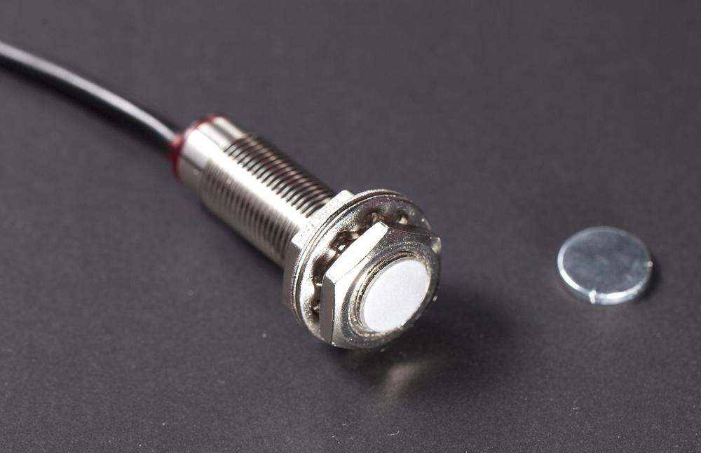
Experiment: Hall Switch
A Hall switch (Figure 10-9) detects if a magnet is nearby. They are often used in measuring how fast a wheel spins. Before GPS, many bike speedometers used Hall switches.
As you bring a magnet near the Hall switch, the code in this experiment prints “switch triggered.”
There are many Hall switches available from different manufactures. We used an affordable and robust Hall Magnetic Sensor (part number 141363) from http://dx.com. That sensor has a nice built-in LED that lights up when a magnet is near. It has weird wire colors: black is data (yes, black goes to D2 rather than the usual GND), blue is ground, and brown is +5 V.
Hall Switch Code and Connection for Arduino
Figure 10-10 shows the wiring diagram for Arduino. Wire it up as shown, and then run the code shown in Example 10-7.

// hall_switch.ino - write to serial if magnet triggers the switch// (c) BotBook.com - Karvinen, Karvinen, ValtokariintswitchPin=2;voidsetup(){Serial.begin(115200);pinMode(switchPin,INPUT);digitalWrite(switchPin,HIGH);}voidloop(){intswitchState=digitalRead(switchPin);//if(switchState==LOW){Serial.println("YES, magnet is near");}else{Serial.println("no");}delay(50);}
-
It’s a simple digital switch, like a button.
Hall Switch Code and Connection for Raspberry Pi
Figure 10-11 shows the circuit for Raspberry Pi. Hook everything up as shown, and then run the code shown in Example 10-8.

# hall_switch.py - write to screen if magnet triggers the switch# (c) BotBook.com - Karvinen, Karvinen, Valtokariimporttimeimportbotbook_gpioasgpio#defmain():switchPin=3# has internal pull-up #gpio.mode(switchPin,"in")while(True):switchState=gpio.read(switchPin)#if(switchState==gpio.LOW):"switch triggered"time.sleep(0.3)if__name__=="__main__":main()
-
Make sure there’s a copy of the botbook_gpio.py library in the same directory as this program. You can download this library along with all the example code from http://botbook.com. See GPIO Without Root for information on configuring your Raspberry Pi for GPIO access.
-
To avoid a floating pin, you need a pull-up resistor. Fortunately, pull-ups are included on the Raspberry Pi’s GPIO pins 2 and 3.
-
A Hall switch is a simple digital switch sensor, so it works like a button.
Test Project: Solar Cell Web Monitor
Turn your Raspberry Pi into a web server and monitor the voltage of your solar cells remotely (Figure 10-12).

What You’ll Learn
In the Solar Cell Web Monitor project, you’ll learn how to:
- Measure voltage of your solar cells, and then report it on your own web server.
- Turn the Raspberry Pi into a web server—using the most popular web server in the world!
- Create timed tasks using the cron scheduler that keep running even if Raspberry is rebooted.
- Draw graphs with Python matplotlib.
Big, public web servers use many of the same techniques you learn here. We teach Apache and cron to Linux students who work on servers, so these techniques aren’t specific to embedded systems or robots.
Connecting Solar Cells
Do you still remember IKEA’s Solvinden lamp, which we used to build Chameleon Dome? In this project we’re going to use the leftover solar panels from it. If you didn’t use Solvinden in the first place, just adjust these instructions to suit the solar cells you are using. First, desolder the red wire marked in Figure 10-13.

You don’t need IKEA’s Solvinden lamp to build this. Just connect a solar cell according to the circuit diagram Figure 10-17. Because you’re using a current sensor with a maximum measured voltage of 13.6 V, make sure the solar cell or panel doesn’t put out more than 13.6 V. If you’re using a different solar cell, it probably has power leads, so you won’t need to follow the Solvinden disassembly steps.
Cut the jumper wires as shown in Figure 10-14 and solder them to the current sensor and to the solar cells as shown in Figure 10-15. The final product is shown in Figure 10-16.


Use the AttoPilot Compact DC Voltage and Current Sense code you tried earlier to test that your connection works. Use a flashlight to see how much current your solar panels collect. We got from 1-3 V from ours.
Hook up the Raspberry Pi to the current sensor as shown in Figure 10-17.

Turn Raspberry Pi into Web Server
Apache is one of the most popular web servers on the planet. According to the Netcraft web server survey, at many times in its lifetime, it has been more popular than all competing web servers together.
These web server instructions have a lot of explanations. If you are well-versed in Linux, you can just read the commands to get the job done in a couple of minutes.
To turn Raspberry Pi into a web server, you must install Apache. The steps to install Apache on Raspberry Pi are exactly the same as you would use when installing Apache on a physical server, virtual server, or a development laptop. If you are using Debian or Ubuntu on your laptop, you can try the same steps there.
On your Raspbian desktop, open the command-line interface (LXTerminal; you’ll find the icon on the left side of the desktop).
Update the list of available packages, and then install Apache:
$ sudo apt-get update
$ sudo apt-get -y install apache2
The web server is now installed and running. Try it out with a web browser, such as Midori. The Midori icon is on the left side of the desktop. Browse to
http://localhost/
Do you see a web page? “It works”? Congratulations, you now run a web server:
Finding Your IP Address
To access your web server from other computers, check your IP address:
$ ifconfig
Look for inet addr in the output. It’s usually under the eth0 or wlan0 interface.
Your public IP address is not 127.0.0.1. That’s localhost address, and every computer refers to itself as localhost.
You can try browsing to this address, too. Just open Midori, and type “http://” and the IP address as the URL. For example, http://10.0.0.1. Obviously, you must use your own address.
This address can also work on your local network. You can try browsing to the address with other computers on your network. Can you see your web server from your laptop or desktop?
Making Your Home Page on Raspberry Pi
It’s easy to set up and maintain a web page if you create it as a user home page. There are two steps: enabling users to make home pages and making the home pages.
Allow users to make home pages. As this changes system-wide settings, you need to use sudo. The following commands enable the Apache user directory module, and then restart Apache:
$ sudo a2enmod userdir
$ sudo service apache2 restart
Now it’s time to create your (pi) home page directory. This doesn’t require sudo privileges. The name of your home page directory, public_html, consists of the word “public”, underscore (“_”), and the word “html”. It must be written correctly.
$ cd /home/pi/
$ mkdir public_html
If you want, you can make a test page:
$ echo "botbook">/home/pi/public_html/hello.txt
Try it with the Midori web browser:
http://localhost/~pi/hello.txt
If you feel adventurous, try your IP address instead of localhost. You could even try visiting your page from your desktop computer on the same network.
Well done—you have now turned Raspberry Pi into a web server! And you’ve already got a home page there. Let’s look at the program, and then we’ll set it up to run periodically.
Solar Panel Monitor Code and Connection for Raspberry Pi
This code requires matplotlib, a great free Python library for mathematical graphing. Install it with these commands:
$ sudo apt-get update
$ sudo apt-get -y install python-matplotlib
Another useful tool for data visualization is Plotly. You can see an example project at Instructables.
Running voltage_record.py once records a new data point and creates one graph, and then exits. No loop is needed, because you’ll see how to use cron to run the program every five minutes.
The measurement history is kept in /home/pi/record.csv.
The generated plot file is put into /home/pi/public_html/history.png. Because you’ve already installed Apache, this file is published at the URL http://localhost/~pi/history.png. To visit that page from another device, you need to replace localhost with your Raspberry Pi’s IP address.
# voltage_record.py - record voltage from solar cell and print history to png# (c) BotBook.com - Karvinen, Karvinen, Valtokariimporttimeimportosimportmatplotlib#matplotlib.use("AGG")#importmatplotlib.pyplotaspltimportnumpyfromdatetimeimportdatetimefromdatetimeimportdatefromdatetimeimporttimedeltaimportattopilot_voltage#importshelvehistoryFile="/home/pi/record"#plotFile="/home/pi/public_html/history.png"#defmeasureNewDatapoint():returnattopilot_voltage.readVoltage()#defmain():history=shelve.open(historyFile)#ifnothistory.has_key("x"):#history["x"]=[]#history["y"]=[]history["x"]+=[datetime.now()]#history["y"]+=[measureNewDatapoint()]#now=datetime.now()#sampleCount=24*60/5history['x']=history["x"][-sampleCount:]history['y']=history["y"][-sampleCount:]plot=plt.figure()#plt.title('Solar cell voltage over last 24h')plt.ylabel('Voltage V')plt.xlabel('Time')plt.setp(plt.gca().get_xticklabels(),rotation=35)plt.plot(history["x"],history["y"],color='#4884ff')#plt.savefig(plotFile)#history.close()#if__name__=='__main__':main()
-
This library must be installed as directed earlier in this section.
-
AGG (Anti-Grain Geometry) is a good matplotlib backend for saving pixel graphics (PNG).
-
The example you created earlier must be in an attopilot_voltage/ directory that’s stored in the same directory as this program (voltage_record.py). See Experiment: Voltage and Current.
-
This is the “shelve” file, where numerical data is stored. Python’s
shelvefunction (which you’ll see in a moment) makes it very easy to store values.-
The plot (a PNG image) to be created. To publish it as a web page, we put it in a folder that’s served up by the Apache web server.
-
This is the actual measurement command. To measure anything else, just change this command.
-
Open the history file. The file is created automatically if needed.
-
If our variables aren’t in the shelve yet…
-
…create them. The shelve history is a dictionary. The keys x and y store one list each.
-
Append timestamp to x. Notice how we don’t have to care about date formatting or parsing.
-
Append measured value to y. The x and y dictionaries are completely different, but values with the same index are related. For example, the data point stored in y[12] is from the time stored in x[12].
-
This stanza drops records older than 24 hours. A simpler, alternative way would be to just store 100 data points and cut after that.
-
Create a new matplotlib plot to draw on.
-
Draw the actual graph.
-
Save the whole plot as a PNG image.
-
Close the shelve to write our values to disk.
Timed Tasks with Cron
Cron is our favorite way of performing timed tasks. Even if your Raspberry Pi shuts down, cron tasks are resumed after reboot.
First make sure that you can run the Python program on the command line, with full path. Use the path to wherever you have downloaded or saved voltage_record.py (see Example 10-9).
$ python /home/pi/voltage_record/voltage_record.py
Don’t you remember where you put voltage_record.py? Run this: cd /home/pi; find -iname voltage_record.py.
If it executes normally, it’s time to add it as a timed task to cron. Edit your user cron file with this:
$ crontab -e
Add the following as the last lines of the file:
*/5 * * * * /home/pi/voltage_record/voltage_record.py
*/1 * * * * touch /tmp/botbook-cron
Save the file. If you edited it with nano, press Control-X, y, then Enter to save.
The first line tells cron to run the program whenever minutes are divisible by 5 (:00, :05…), ignoring hour, day of month, month, and day of week.
The second line just creates an empty file /tmp/botbook-cron every minute. It’s for checking up on cron, and you can delete this line later if you want. Wait for a minute, and then check if the file is there:
$ ls /tmp/botbook*
/tmp/botbook-cron
Did ls show your file? Well done! You successfully added a timed task to cron.
Whenever you want Raspberry Pi to automatically do something, use cron. Even if the power is cut, the timed tasks are run again when you boot up the Raspberry Pi.
What’s Next?
You have now played with electricity. Your gadgets can measure voltage and current, even at levels that would break your microcontroller board if connected directly. Magnetic fields can be detected simply, as a Hall switch detects a magnet, or in an advanced way as you did with the three-dimensional, tilt-corrected compass.
The solar cell web monitor you built can be adapted to any sensor project. Simply by changing the measurement function, you can store data from any sensor. In your project, you published the graph to the Web. Try adding password protection or even use ssh to view the graph for projects requiring more secrecy.
In the next chapter, you move from electromagnetism to sound waves. It’s time to give ears to your gadgets!