Chapter 10

mental ray Shading Techniques

A shader is a rendering node that defines the material qualities of a surface. When you apply a shading node to your modeled geometry, you use the shader’s settings to determine how the surface will look when it’s rendered. Will it appear as shiny plastic? Rusted metal? Human skin? The shader is the starting point for answering these questions. Shading networks are created when one or more nodes are connected to the channels of the shader node. These networks can range from simple to extremely complex. The nodes that are connected to shaders are referred to as textures. They can be image files created in other software packages or procedural (computer-generated) patterns, or they can be special nodes designed to create a particular effect.

The Autodesk® Maya® software comes with a number of shader nodes that act as starting points for creating various material qualities. The mental ray® plug-in also comes with its own special shader nodes that expand the library of available materials. Since the mental ray rendering plug-in is most often used to create professional images and animations, this book emphasizes mental ray techniques. You’ll learn how to use mental ray shaders to create realistic images.

In this chapter, you will learn to:

  • Understand shading concepts
  • Apply reflection and refraction blur
  • Use basic mental ray shaders
  • Apply the car paint shader
  • Use the mia materials
  • Render contours

Shading Concepts

Shaders are sets of specified properties that define how a surface reacts to lighting in a scene. A mental ray material is a text file that contains a description of those properties organized in a way that the software understands. In Maya, the Hypershade provides you with a graphical user interface so that you can edit and connect shaders without writing or editing the text files themselves.

The terms shader and material are synonymous; you’ll see them used interchangeably throughout this book and the Maya interface. mental ray also uses shaders to determine properties for lights, cameras, and other types of render nodes. For example, special lens shaders are applied to cameras to create effects such as depth of field.


The mental ray Plug-in
mental ray is a rendering plug-in that is included with Maya. It is a professional-quality photorealistic renderer used throughout the industry in film, television, architectural visualization, and anywhere photorealism is required.
Learning mental ray takes time and practice. Even though it’s a plug-in, you’ll find that it is as deep and extensive as Maya itself. mental ray includes a library of custom shading nodes that work together to extend the capabilities of mental ray. There are a lot of these nodes—many more than can be covered in this book.
When approaching mental ray as a rendering option, you can quickly become overwhelmed by the number of shading nodes in the mental ray section of the Hypershade. When these shading nodes are coupled with the mental ray–specific attributes found on standard Maya nodes, it can be difficult to know what to use in a particular situation. Think of mental ray as a large toolkit filled with a variety of tools that can be used in any number of ways. Some tools you’ll use all the time, some you’ll need only for specific situations, and some you may almost never use. You’ll also find that, over time, as your understanding of and experience with mental ray grows, you may change your working style and use particular nodes more often. As you work with mental ray, expand your knowledge and experience through study and experimentation.
In this chapter, you’ll be introduced to the most commonly used nodes, which will make you more comfortable using them in professional situations. There should be enough information in this chapter to give the everyday Maya user a variety of options for shading and rendering using mental ray. If you decide that you’d like to delve deeper into more advanced techniques, we recommend reading the mental ray shading guide that is part of the Maya documentation, as well as Boaz Livny’s excellent book mental ray for Maya, 3ds Max, and XSI (Sybex, 2008).
Before starting this chapter, make sure that you are familiar with using and applying standard Maya shaders, such as the Lambert, Blinn, Phong, Ramp, Surface, and Anisotropic shaders. You should be comfortable making basic connections in the Hypershade and creating renders in the Render View window. You should understand how to use Maya 2D and 3D textures, such as Fractal, Ramp, and Checker. Review Chapter 9, “Lighting with mental ray,” for background on lighting with mental ray. Many of the issues discussed in this chapter are directly related to lighting and mental ray lighting nodes.

This section focuses on shaders applied to geometry to determine surface quality. Three key concepts that determine how a shader makes a surface react to light are diffusion, reflection, and refraction. Generally speaking, light rays are reflected or absorbed or pass through a surface. Diffusion and reflection are two ways in which light rays bounce off a surface and back into the environment. Refraction refers to how a light ray is bent as it passes through a transparent surface. This section reviews these three concepts as well as other fundamentals that are important to understand before you start working with the shaders in a scene.

certobjective.eps

Maya Standard Shaders and mental ray Materials
The Maya standard shaders are found in the left list in the Hypershade window when you click the Surface heading under Maya (as shown here). The most often used standard shaders are Blinn, Lambert, Phong, Phong E, and Anisotropic. You can use any of these shaders when rendering with mental ray.
c10uf001.tif
The mental ray materials (also referred to as shaders) are found in the left list in the Hypershade window when you click Materials under mental ray (as shown here). The shaders will work only when rendering with mental ray.
c10uf002.tif
This chapter will discuss some aspects of working with the standard Maya shaders, but for the most part it will focus on the most often-used mental ray shaders. If you are unfamiliar with the standard shaders, we recommend you review the Maya documentation.

Diffusion

Diffusion describes how a light ray is reflected off a rough surface. Think of light rays striking concrete. Concrete is a rough surface covered in tiny bumps and crevices. As a light ray hits the bumpy surface, it is reflected back into the environment at different angles, which diffuse the reflection of light across the surface (see Figure 10-1).

Figure 10-1 Light rays that hit a rough surface are reflected back into the environment at different angles, diffusing light across the surface.

c10f001.tif

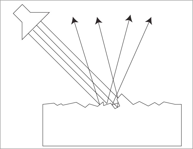
You see the surface color of the concrete mixed with the color of the lighting, but you generally don’t see the reflected image of nearby objects. A sheet of paper, a painted wall, and clothing are examples of diffuse surfaces.

In standard Maya shaders, the amount of diffusion is controlled using the Diffuse slider. As the value of the Diffuse slider is increased, the surface appears brighter because it is reflecting more light back into the environment.

Reflection

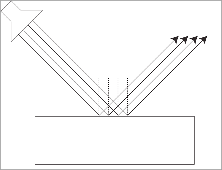
When a surface is perfectly smooth, light rays bounce off the surface and back into the environment. The angle at which they bounce off the surface is equivalent to the angle at which they strike the surface—this is the incidence angle. This type of reflection is known as a specular reflection. You can see the reflected image of surrounding objects on the surface of smooth, reflective objects. Mirrors, polished wood, and opaque liquids are examples of reflective surfaces. A specular highlight is a reflection of the light source on the surface of the object (see Figure 10-2).

Logically, smoother surfaces, or surfaces that have a specular reflectivity, are less diffuse. However, many surfaces are composed of layers (think of glossy paper) that have both diffuse and specular reflectivity.

Figure 10-2 Light rays that hit a smooth surface are reflected back into the environment at an angle equivalent to the incidence of the light angle.

c10f002.tif

A glossy reflection occurs when the surface is not perfectly smooth but not so rough as to diffuse the light rays completely. The reflected image on a surface is blurry and bumpy and otherwise imperfect. Glossy surfaces can represent those surfaces that fit between diffuse reflectivity and specular reflectivity.

Refraction

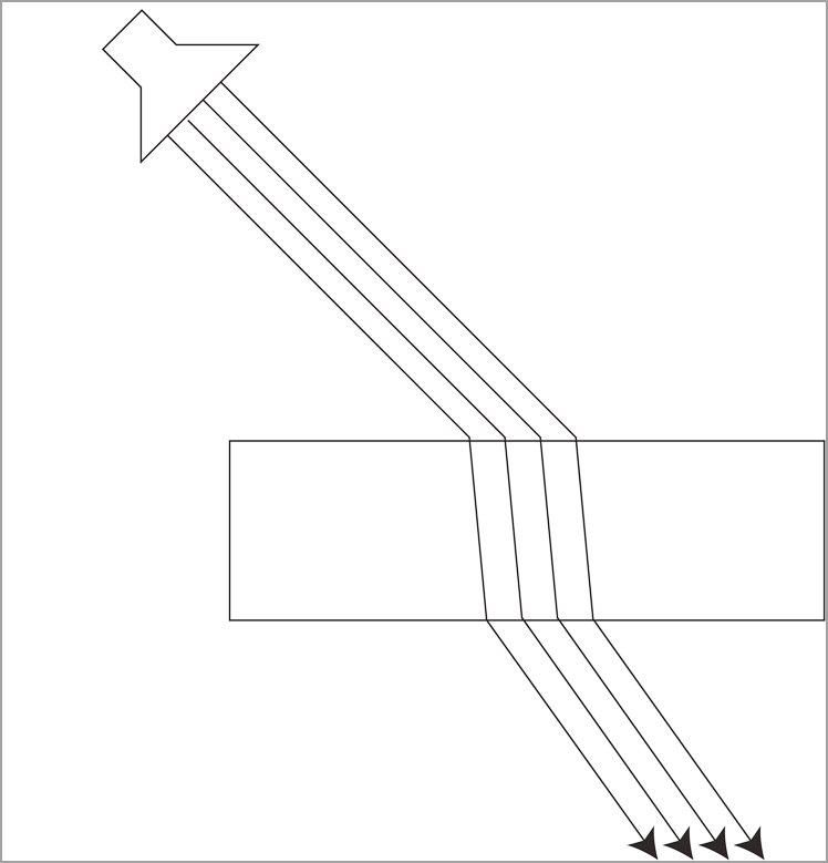
A transparent surface can change the direction of the light rays as they pass through the surface (see Figure 10-3). The bending of light rays can distort the image of objects on the other side of the surface. Think of an object placed behind a glass of water. The image of the object as you look through the glass of water is distorted relative to an unobstructed view of the object. Both the glass and the water in the glass bend the light rays as they pass through.

Shaders use a refractive index value to determine how refractions will be calculated. The refraction index is a value that describes the amount by which the speed of the light rays is reduced as it travels through a transparent medium, as compared to the speed of light as it travels through a vacuum. The reduction in speed is related to the angle in which the light rays are bent as they move through the material. A refraction index of 1 means the light rays are not bent. Glass typically has a refractive index between 1.5 and 1.6; water has a refractive index of 1.33.

If the refracting surface has imperfections, this can further scatter the light rays as they pass through the surface. This creates a blurry refraction.

Refraction in Maya is available only when ray tracing is enabled (mental ray uses ray tracing by default). The controls for refraction are found in the Raytrace section of the Attribute Editor of standard Maya shaders. A shader must have some amount of transparency before refraction has any visible effect.

Figure 10-3 Refraction changes the direction of light rays as they pass through a transparent surface.

c10f003.tif

The Fresnel Effect

The Fresnel effect is named for the nineteenth-century French physicist Augustin-Jean Fresnel (pronounced with a silent s). This effect describes the amount of reflection and refraction that occurs on a surface as the viewing angle changes. The glancing angle is the angle at which you view a surface. If you are standing in front of a wall, the wall is perpendicular, and thus the glancing angle is 0. If you are on the beach looking out across the ocean, the glancing angle of the surface of the water is very high. The Fresnel effect states that as the glancing angle increases, the surface becomes more reflective than refractive. It’s easy to see objects in water as you stare straight down into water (low glancing angle); however, as you stare across the surface of water, the reflectivity increases, and the reflection of the sky and the environment makes it increasingly difficult to see objects in the water.

Opaque, reflective objects also demonstrate this effect. As you look at a billiard ball, the environment is more easily seen reflected on the edges of the ball as they turn away from you than on the parts of the ball that are perpendicular to your view (see Figure 10-4).

Figure 10-4 A demonstration of the Fresnel effect on reflective surfaces: the reflectivity increases on the parts of the sphere that turn away from the camera.

c10f004.tif

Anisotropy

Anisotropic reflections appear on surfaces that have directionality to their roughness, which causes the reflection of light to spread in one direction more than another. When you look at the surface of a compact disc, you see the tiny grooves that are created when data is written to the disc to create the satin-like anisotropic reflections. Brushed metal, hair, and satin are all examples of materials that have anisotropic specular reflections.

The resulting stretch or compression of an anisotropic reflection is defined in U and V directions. Anisotropy works in conjunction with the UV coordinates defined on a piece of geometry. (UV texture layout will be covered in Chapter 11, “Texture Mapping”).

Creating Blurred Reflections and Refractions Using Standard Maya Shaders

Standard Maya shaders, such as the Blinn and Phong shaders, take advantage of mental ray reflection and refraction blurring to simulate realistic material behaviors. These options are available in the mental ray section of the shader’s Attribute Editor. As you may have guessed, since these attributes appear in the mental ray rollout of the shader’s Attribute Editor, the effect created by these settings will appear only when rendering with mental ray. They do not work when using other rendering options, such as Maya Software.

Reflection Blur

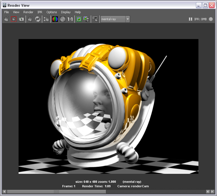
Reflection blur is easy to use, and it is available for any of the standard Maya shaders that have reflective properties, such as Blinn, Phong, Anisotropic, and Ramp. This exercise demonstrates how to add reflection blur to a Blinn shader. This scene contains a space helmet model above a checkered ground plane.

1. Open the reflectionBlur.ma file from the chapter10scenes folder at the book’s web page (www.sybex.com/go/masteringmaya2014).
2. In the Outliner, select the shield surface. This is the glass face shield at the front of the helmet. Assign a Blinn shader to the shield, and name the shader shieldShader.

Quickly Assign a Shader to a Surface
There are several ways to assign a shader to a surface quickly:
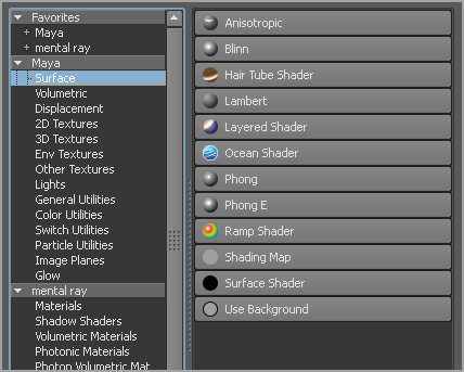
  • Many standard Maya shaders are available in the Rendering shelf. You can select an object in a scene and click one of the shader icons on the shelf. This creates a new shader and applies it to the selected object at the same time. The names of the shaders appear on the help line in the lower left of the Maya interface.
  • Another way to apply a shader is to select the object in the viewport window, right-click it, and choose Assign New Material from the bottom end of the marking menu. This will open a window with a list of material bases.
  • You can select the object, switch to the Rendering menu set, and choose Lighting/Shading ⇒ Assign New Material.

3. In the Common Material attributes rollout of the shieldShader, set Diffuse to 0, and set Transparency to white so that you can see inside the helmet.
4. In the Specular Shading rollout, set Specular Color to white and set Reflectivity to 1.
certobjective.eps
5. Change Eccentricity to 0.2 and Specular Roll Off to 0.8. The Eccentricity setting controls the intensity of the “hot spot” of the specular highlight. The Specular Roll Off setting controls the surface’s ability to reflect its surroundings; however, when raytracing this has no effect on the reflection. In this raytraced scene, Specular Roll Off has been raised to decrease the softness of the specular highlight, giving a more glasslike appearance to the shield.
6. The mental ray renderer has already been selected in this scene. Render the scene in the Render View window from the renderCam camera (see the left side of Figure 10-5).
7. Store the image in the Render View window.
8. Scroll down in the Attribute Editor for shieldShader, expand the mental ray rollout, and increase Mi Reflection Blur to 8 (see Figure 10-6).
9. Create another test render, and compare this to the render in the previous step (see the right side of Figure 10-5).

Figure 10-5 The reflection on the face shield is blurred in the right image.

c10f005.tif

Figure 10-6 The Reflection Blur settings are in the mental ray rollout of the shader’s Attribute Editor.

c10f006.tif

You can see how the reflection of the checkered pattern on the face shield now appears blurred.

Reflection Blur Limit sets the number of times the reflection blur itself is seen in other reflective surfaces. Increasing the Reflection Rays value increases the quality of the blurring, making it appear finer. Notice that the reflection becomes increasingly blurry as the distance between the reflective surface and the reflected object increases.

Many surfaces are more reflective than you may realize. An unpolished wooden tabletop or even asphalt can have a small amount of reflection. Adding a low reflectivity value plus reflection blurring to many surfaces increases the realism of the scene.

Refraction Blur

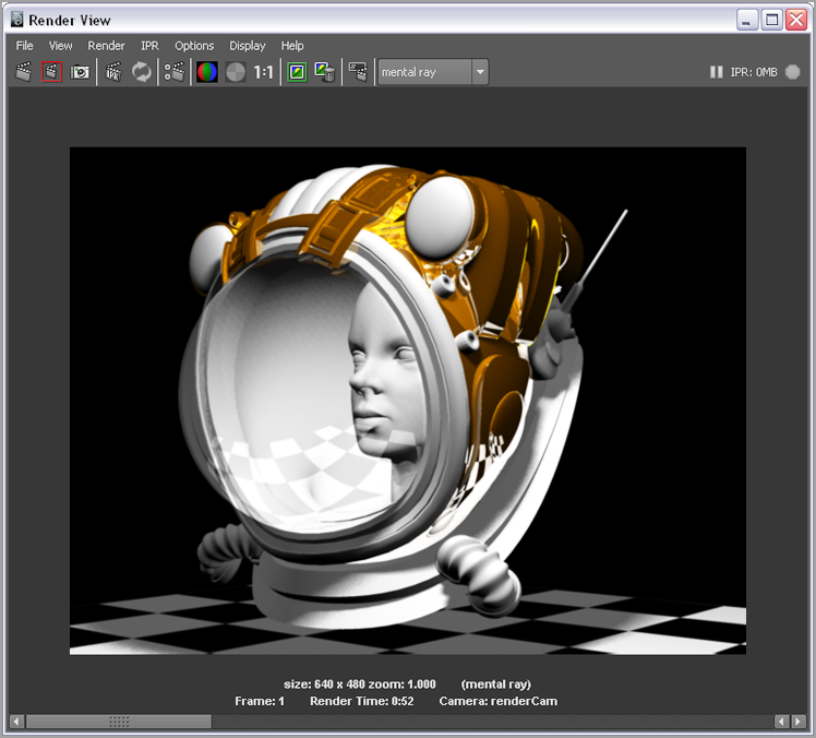
Refraction blur is similar to reflection blur. It blurs the objects that appear behind a transparent surface that uses refraction. This gives a translucent quality to the object.

1. Continue with the scene from the previous section.
2. Set the Mi Reflection Blur value of the shieldShader back to 0. Set Reflectivity to 0 as well. This way, you’ll clearly be able to see how refraction blur affects the shader.
3. In the Attribute Editor for the shieldShader, expand the Raytrace Options rollout, and activate the Refractions option. Set Refractive Index to 1.2.
4. Render the scene from the renderCam camera, and store the image in the Render View window (see the left image in Figure 10-7). The image of the face appears distorted behind the shield object because of the refraction of light as it passes through the glass.

Figure 10-7 The image of the face is refracted by the surface of the face shield (left image). The refracted image is then blurred (right image).

c10f007.tif
5. Expand the mental ray section in the shieldShader’s Attribute Editor. Set Mi Refraction Blur to 2, and create another test render (see the right image in Figure 10-7).
6. Save the scene as reflectionBlur_v02.ma.

To see a version of the scene, open the reflectionBlur_v02.ma file from the chapter10scenes folder at the book’s web page.

Refraction Blur Limit sets the number of times the refraction blur itself will be seen in refractive surfaces. Increasing the value of Refraction Rays increases the quality of the blurring, making it appear finer.

certobjective.eps

Interactive Photorealistic Render Preview
Interactive Photorealistic Render (IPR) preview is a mode that can be used in the Render View window. When you create a render preview using the special IPR mode, any changes you make to a shader or the lighting, or even some modeling changes in the scene, automatically update the Render View window, allowing you to see a preview of how the changes will look interactively. IPR works very well with mental ray; in fact, it supports more rendering features for mental ray than for Maya Software.
In addition, Maya 2014 offers a progressive rendering mode for IPR. This mode begins rendering with a low sampling rate and progressively increases the rate until the render reaches its final result. This rendering mode allows for fast previews without having to commit to a lengthy render time.
The workflow for creating an IPR render in mental ray is slightly different from the one for creating a Maya Software IPR. To create an IPR render, follow these steps:
1. Select the viewport you wish to render by clicking an empty portion of the viewport menu bar. Open the Render View by using the IPR button (labeled IPR at the right side of the status line).
2. Select a region by drawing a region box over the parts of the image you want to tune. The region renders. To avoid demanding too much memory for IPR, keep the region box as small as possible. To enable Progressive Mode, you must use Unified Sampling and set the Progressive Mode option to IPR Only in the Sampling drop-down under the Quality tab.
3. Make changes to the materials and the lighting; you’ll see the image in the selected region box update as you make the changes.
4. When you are done with your tuning, stop IPR from constantly updating by clicking the IPR stop sign icon in the upper right of the Render View.
Most, but not all, mental ray features are supported by IPR. Occasionally you’ll need to click the IPR button to update the render if IPR gets out of sync (or choose IPR ⇒ Refresh IPR Image from the menu in the Render View window). The IPR render is a close approximation of the final render; be aware that what you see in the IPR render may look slightly different in the final render.

Basic mental ray Shaders

mental ray has a number of shaders designed to maximize your options when creating reflections and refractions, as well as blurring these properties. Choosing a shader should be based on a balance between the type of the material you want to create and the amount of time and processing power you want to devote to rendering the scene.

This section looks at a few of the shaders available for creating various types of reflections and refractions. These shaders are by no means the only way to create reflections and refractions. As discussed in previous sections, standard Maya shaders also have a number of mental ray–specific options for controlling reflection and refraction.

Once again, remember to think of mental ray as a big toolbox with lots of options. The more you understand about how these shaders work, the easier it will be for you to decide which shaders and techniques you want to use for your renders.

DGS Shaders

Diffuse Glossy Specular (DGS) shaders have simple controls for creating different reflective qualities for a surface as well as additional controls for transparency and refraction. The reflections and refractions created by this shader are physically accurate, meaning that, at render time, mental ray simulates real-world light physics as much as possible to create the look seen in the render.

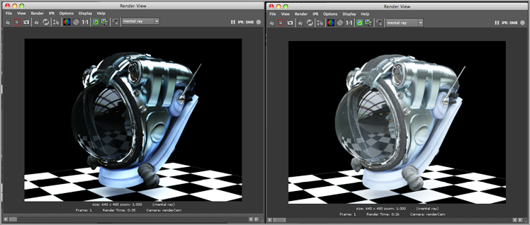
The scene has a simple light setup. The key lighting is provided by a mental ray area light, which can be seen as a specular highlight on the orange metal of the helmet and on the glass face shield. The fill lighting is supplied by two directional lights; these lights have their specularity turned off so that they are not seen as reflections on the surface of the helmet (see Figure 10-8).

Figure 10-8 The space helmet rendered with simple lighting and standard Maya shaders

c10f008.tif

The helmet uses standard Maya shaders. The metal of the helmet uses an orange Blinn, the face shield uses a transparent Blinn, and the helmet details and the woman’s head use Lambert shaders. The grainy quality of the shadows results from the low sampling level set for the area light. By keeping the samples low, the image renders in a fairly short amount of time. The reflection of the checkerboard plane beneath the helmet is clearly seen in the metal of the helmet and on the face shield.

1. Open the helmet_v01.ma scene from the chapter10scenes folder at the book’s web page.
2. Open the render view, and create a render using the renderCam camera.
3. Store the render in the Render View window.
4. Open the Hypershade editor. In the list on the left side of the Hypershade editor, select Legacy Materials under the mental ray heading.
5. Click the dgs_material button, about halfway down the material list, twice to create two DGS material nodes.
6. Name the first one helmet_dgs and the second shield_dgs.
7. In the Outliner, select the group labeled helmetSurfaces.
8. In Hypershade, right-click the helmet_dgs shader, and choose Assign Material To Selection from the marking menu. This assigns the material to all the objects in the group.
9. In the Outliner, select the shield surface. In the Hypershade, right-click the shield_dgs material, and choose Assign Material To Selection from the marking menu.
10. In the Hypershade, select the helmet_dgs material and open its Attribute Editor.
11. Set the Diffuse color to bright orange. Set Glossy to black and Specular to white.
12. In the Hypershade, select the shield_dgs material.
13. Set Transp (transparency) to 0.8. Set Glossy to black and Specular to white.
14. In the render view, render the scene from the renderCam camera. Compare this render to the previous render. Immediately, you’ll notice a lot of strange things going on with the materials you just applied (see Figure 10-9).

If you compare Figure 10-9 to Figure 10-8, you should notice a few details:

  • The surfaces are reflective; however, there is no specular highlight (reflection of the light source) on either the helmet surfaces or the glass shield in Figure 10-9.
  • The shadow of the face shield that falls on the checkered floor is not transparent in Figure 10-9, but it is transparent in Figure 10-8.

Figure 10-9 The helmet and face shield surfaces have DGS shaders applied.

c10f009.tif

Let’s look at how to solve these problems. The shader is meant to be physically accurate. The Specular attribute refers to the reflectivity of the shader. In standard Maya shaders, reflectivity and specularity are separated (however, increasing one affects the intensity of the other). But in the DGS shader attributes, the Specular channel controls the reflection of visible objects, so a light source must be visible to be seen in the specular reflections.

1. Select the area light in the Hypershade, and open its Attribute Editor.
2. In the areaLightShape1 tab, expand the mental ray attributes and activate the Visible option.
3. Render the scene again. This time you can see a reflection of the light in the surfaces. You can clearly see that the light is square-shaped.

Glossy reflections, on the other hand, automatically render the reflection of a light source regardless of whether the light source is set to Visible. The Glossy attribute on the DGS shader controls how reflections are scattered across the surface of an object. The term specular highlight with regard to shading models implies a certain amount of glossiness. Understandably, it’s confusing when talking about specular reflections and specular highlights as two different things. The bottom line is this: to make a specular highlight appear in a DGS shader, either the light has to be visible when the Specular attribute is greater than 0 and Glossy is set to 0 or the Glossy setting must be greater than 0 (that is, not black).

Glossy reflections can be blurry or sharp. To control the blurriness of a glossy reflection, you need to adjust the Shiny setting. Lower Shiny values create blurry reflections; higher Shiny values create sharp reflections.

1. Select the helmet_dgs shader, and open its Attribute Editor. Enter the following settings:
Glossy: A medium gray
Specular color: Black
Shiny: 10
2. Create another render. This time the surface of the helmet appears more like painted metal and less like a mirror (the upper-left image in Figure 10-10).

Figure 10-10 Rendering using different settings for the DGS materials applied to the helmet metal and face shield

c10f010.tif
The Shiny U and Shiny V settings control the blurriness of the glossy reflection when Shiny is set to 0. Using these settings, you can create an anisotropic type of reflection.
3. The U and V values control the direction of the anisotropic reflections across the surface. For best results, set one value higher than the other:
Shiny: 0
Shiny U value: 3
Shiny V value: 10
4. Create another render; the helmet now appears more like brushed metal (the upper-right image in Figure 10-10).

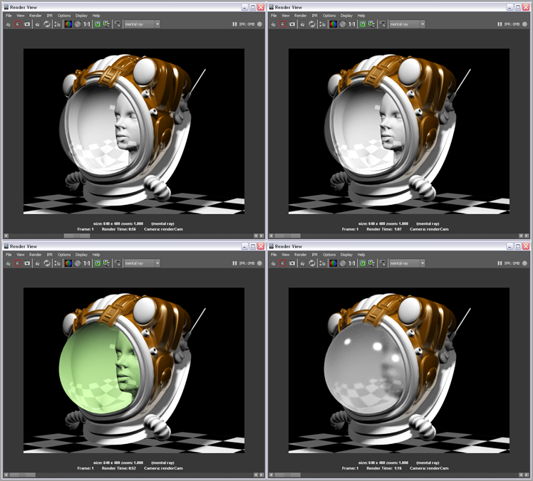
The Shiny U and Shiny V settings simulate the anisotropic reflections on the material by stretching the reflection along the U or V direction. In this case, this is not physically accurate and does not simulate how tiny grooves in the surface affect the reflection.


Isotropic and Anisotropic Specular Reflections
Isotropic and anisotropic both refer to a glossy specular highlight caused by microfacets on a surface. These tiny imperfections scatter reflected highlights, giving a glossy or blurry edge to highlights. Isotropic surfaces have a random order to the direction of the microfacets on the surface; anisotropic surfaces have microfacets that all run in a similar direction, which spread the specular highlights in a particular direction.

When rendering transparent surfaces using the DGS shader, the Specular, Glossy, Transparency, and Refraction settings all work together to create the effect. For transparency to work, the shader must have a Transparency setting higher than 0 and either a Specular or a Glossy setting greater than 0. If Transparency is set to 1, and both Specular and Glossy are set to black, the surface will render as opaque, the same as if Transparency were set to 0.

The Specular color can be used to color the transparent surface, and the Glossy setting can be used (along with the Shiny settings) to create the look of a translucent material, such as plastic, ice, or frosted glass:

1. Select the shield_dgs material. Set the Specular color to a light green, and the Glossy to black. Also remove the anisotropic shine by setting Shiny U and V to 0.
2. Set Transparency to 0.8.
3. Set Index Of Refraction to 1.1. This makes the glass appear thicker because the light rays are bent as they pass through the glass.
4. Create another test render. Notice that the green specular color tints both the objects behind the glass as well as the reflections on the surface (see the lower-left image in Figure 10-10; the image is in black and white, but you can clearly see the effect of the refraction setting).
5. To create the look of frosted glass, enter these settings:
Diffuse: Light gray
Specular: Black
Glossy: Light gray
Shiny: 20
Transparency: 0.8
Index Of Refraction: 1.2
6. Create another test render to see the result (the lower-right image in Figure 10-10).
7. Save the scene as helmet_v02.ma.

A few details are worth noting about using the Glossy settings:

  • Specular reflections of all the lights in the scene are visible on the surface when Glossy is greater than 0. Notice that the highlights of the two directional lights are visible in the glass even though the Specularity option for both lights is disabled. To avoid this, consider using Global Illumination or Final Gathering to create fill lighting in the scene. (See Chapter 9 for information on these techniques.)
  • Glossy reflections and refractions are physically accurate in that objects close to the refractive or reflective surface will appear less blurry than objects that are farther away.
  • To make an object look more metallic, tint the Glossy color similar to the Diffuse color.
  • Try using textures in the Glossy and Specular channels to create more interesting materials.
  • When using the shader on scenes that employ Global Illumination, you need to create a dgs_material_photon node (found in the Photonic Materials section of the mental ray render nodes of the Hypershade). Attach this shader to the shading group of the original DGS material in the Photon Shader slot, and then use the settings on the dgs_material_photon node to control the shader.
  • You can increase realism further by rendering a separate reflection occlusion pass to use in a composite (render passes are covered in Chapter 12, “Rendering for Compositing”) or plug occlusion textures into the specular and glossy attributes (enable Reflection on the occlusion textures).

To see a finished version of the scene, open the helmet_v02.ma scene from the chapter10scenes folder at the book’s web page.

Dielectric Material

The purpose of the Dielectric material is to simulate the refraction of light accurately as it passes through transparent materials such as glass, water, and other fluids. The term dielectric refers to a surface that transmits light through multiple layers, redirecting the light waves as they pass through each layer.

If you observe a fish in a glass bowl, you’ll see that the light rays that illuminate the fish in the bowl transition from air to glass, then from glass to water, then again from water back to glass, and finally from glass out into the air on the other side. Each time a light ray makes a transition from one surface to another, the direction of the light ray changes. The index of refraction describes the change in the light ray’s direction.

Most standard materials in Maya use a single index of refraction value to simulate the change of direction of the light ray as it is transmitted through the surface. This is not accurate, but it’s usually good enough to create a believable effect. However, if you need to create a more physically accurate refractive surface, the Dielectric material is your best choice. This is because it has two settings for the index of refraction that describes the change of the light ray’s direction as it makes a transition from one refractive surface to the next.

In this exercise, you’ll create a physically accurate rendering of a glass of blue liquid using the Dielectric material. Light will move from the air into glass and then from the glass into the water. The glass is open at the top, so you’ll also need to simulate the transition from air to water. This means you’ll need to use three Dielectric materials: one for air to glass, one for glass to water, and one for air to water. This tutorial is based on Boaz Livny’s discussion of the Dielectric material in mental ray for Maya, 3ds Max, and XSI (Sybex, 2008).

In this scene, a simple glass has been modeled and split into four surfaces, named air_glass1, air_glass2, liquid_glass1, and liquid_air1. Each surface represents one of the three transitions that will be simulated using the Dielectric material. To make this easier to visualize, we applied a colored Lambert shader to each surface. The scene is lit using a single spotlight that casts raytrace shadows.

1. Open glass_v01.ma from the chapter10scenes folder at the book’s web page.
2. Open the Hypershade window. Select the Legacy Materials heading under the mental ray section from the list on the left side of the Hypershade window.
3. In the Legacy Materials section, click the dielectric_material button.
4. Name the new dielectric_material1 node air2GlassShader.
5. Create two more dielectric materials, and name one glass2LiquidShader and the other liquid2AirShader.
6. Apply the air2GlassShader to both the airGlass1 and airGlass2 objects. Apply glass2LiquidShader to the liquid_glass1 object and liquid2AirShader to liquid_air1.
7. Select the air2glassShader, and open its Attribute Editor.
The index of refraction (IOR) for glass is typically 1.5, and the IOR for air is 1. Look at the settings for the air2Glass shader. The Index Of Refraction setting defines the IOR for the material; the Outside Index Of Refraction setting defines the IOR for the medium outside the material. The default settings for the Dielectric material are already set to the proper glass-to-air transition. Index Of Refraction should be set to 1.5, and Outside Index Of Refraction should be set to 1.
8. Set Phong Coefficient to 100, and turn on Ignore Normals.
The Phong Coefficient creates a specular reflection on the glass. The Dielectric material uses the surface normals of the object to create the refraction effect. If you activate the Ignore Normals option, the shader bases the normal direction on the camera view. For a basic glass model such as this one, you can safely use the Ignore Normals feature.
9. Select the glass2LiquidShader, open its Attribute Editor, and enter the following settings:
Index Of Refraction: 1.33 (the IOR of water is 1.33)
Outside Index Of Refraction: 1.5
Phong Coefficient: 100
Ignore Normals: On
10. Click the color swatch next to the Col attribute. This determines the color of the shader. (Why spell out Index Of Refraction in the interface but abbreviate Color? It’s one of the many mysteries of Maya.)
11. In the Color Chooser, use the menu below the color wheel to set the mode to HSV (Hue, Saturation, Value), as shown in Figure 10-11. This is just another way to determine color as opposed to setting RGB (red, green, blue) values. Set the following:

Figure 10-11 Use the menu in the Color Chooser to set the mode to HSV.

c10f011.tif
Hue (H): 180
Sat (S): 0.45
Value (V): 1
12. Select the liquid2AirShader. Set Index Of Refraction to 1.33, and leave Outside Index Of Refraction at 1. Set Phong Coefficient to 100, and turn on Ignore Normals.
13. Select the Col swatch, and use the same HSV values in the Color Chooser that you set in step 11.
14. Open the Render View window, and create a test render from the renderCam camera (see Figure 10-12).

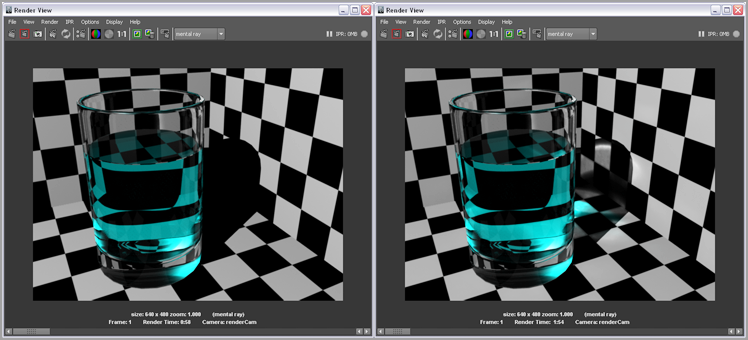
Figure 10-12 Render the glass using the Dielectric material (left image). Add transparent shadows by rendering with caustics (right image).

c10f012.tif
15. Save the scene as glass_v02.ma.

To see a version of the scene, open the glass_v02.ma scene from the chapter10scenes folder at the book’s web page.

You can see that there are differences between the refractions of the various surfaces that make up the glass and the water. Just like the DGS shader, the Dielectric material fails to cast transparent shadows (the left image of Figure 10-12). The best solution for this problem is to enable Caustics. When enabling Caustics with the Dielectric shader, you need to connect a dielectric_material_photon material to the Photon Shader slot of the Shading Group node and enable Caustics. The settings for the dielectric_material_photon material should be the same as the settings for the Dielectric material.

The image on the right of Figure 10-12 shows the glass rendered with Caustics enabled. Using Caustics is explained in Chapter 9. To see an example of this setup, open the dielectricCaustics.ma scene in the chapter10scenes folder at the book’s web page.

mental ray Base Shaders

A number of shaders available in the Hypershade are listed with the prefix mib (mental images base): mib_illum_cooktorr, mib_illum_blinn, and so on. These are the mental ray base shaders. You can think of these nodes as building blocks; you can combine them to create custom mental ray shaders to yield any number of looks for a surface. There are far too many to describe in this chapter, so it’s more important that you understand how to work with them. Descriptions of each node are available in the mental ray user guide that is part of the Maya documentation.

In this exercise, you’ll see how a few of these shaders can be combined to create a custom material for the helmet:

1. Open the helmet_v03.ma scene from the chapter10scenes folder at the book’s web page. This scene currently uses standard Maya shaders applied to the geometry.
2. Open the Hypershade window, and select the Legacy Materials heading under the mental ray section in the list on the left side. Scroll down the list, and you’ll see a number of mib materials toward the bottom (see Figure 10-13).

Figure 10-13 The mental ray base shaders are available in the Legacy Materials section of the Create mental ray Nodes menu.

c10f013.tif
3. Click the mib_illum_cooktorr button to create a Cook-Torrance material, and open its Attribute Editor.
The Cook-Torrance shader creates physically accurate isotropic specular highlighting, meaning that the specular highlights on surfaces are scattered as if the surface were covered with microfacets arranged randomly.
The look of the highlight is created by setting the Specular color to a value greater than 0. The Roughness slider determines the spread of the highlight. The shader has three separate controls to determine the index of refraction for each color channel (red, green, and blue). When light is reflected from the tiny bumps on an isotropic surface, the directionality of each light wave changes. The three IOR sliders allow you to specify this directional change for each color channel. This gives the specular highlight the appearance of color fringing—a slight tint on the edge of the highlight. (This appears as blue fringe in the shader’s preview.) The color fringing around the highlight makes this shader very useful for creating realistic-looking metals.
The Ward (mib_illum_ward) material is similar to the Cook-Torrance but offers more options for creating realistic anisotropic specularity. The Ward material works best on NURBS surfaces; the mib_illum_ward_deriv shader is a little easier to use, giving you two simple sliders to control the direction of the anisotropy along the U and V coordinates of the surface.
4. In the Outliner, select the helmetSurfaces group.
5. In the Hypershade, right-click the mib_illum_cooktorr1 shader, and choose Assign Material To Selection from the marking menu.
6. In the Attribute Editor, use the following settings:
Diffuse: Light orange
Specular: Light gray
Roughness: 0.19
7. To create an orange fringe around the highlight, set the following:
Index Of Refraction, Red: 80
Index Of Refraction, Green: 10
Index Of Refraction, Blue: 8
8. In the Render View window, create a test render using the renderCam camera (Figure 10-14).

If you have a hard time discerning the color in the highlight from the color of the diffuse component, set Diffuse to black and create another test render.

The helmet has a convincing metallic look, but you’ll notice that there are no reflections. To add reflections, you can combine the Cook-Torrance shader with a glossy reflection node:

1. From the list of Legacy Materials on the left side of the Hypershade editor, click the mib_glossy_reflection button.
2. Assign the new mib_glossy_reflection1 node to the helmet surfaces group. This overwrites the Cook-Torrance shader that has been applied.
3. Open the Attribute Editor for the mib_glossy_reflection1 node.
4. From the Hypershade window, MMB-drag the mib_cook_torr1 node from the Hypershade to the Base Material slot of the mib_glossy_reflection1 node (see Figure 10-15).

Figure 10-14 The Cook-Torrance shader creates fairly realistic metallic highlights.

c10f014.tif

Figure 10-15 Connect the Cook-Torrance shader to the Base Material slot of the mib_glossy_reflection1 node.

c10f015.tif
5. Set Reflection Color to white (white sets the shader to maximum reflectivity; darker shades create a less reflective material), and create another render in the Render View window (see Figure 10-16).

Figure 10-16 The combination of the two materials creates a reflective metal for the helmet.

c10f016.tif
6. The default settings create a blurry reflection in the helmet surfaces. To adjust the quality and blurriness of the reflections, increase the Samples value to 32.

The U Spread and V Spread sliders control the glossiness of the reflections, much like the Shiny U and Shiny V settings on the DGS shader. Higher values produce glossier reflections. Using a different value for U than V creates anisotropic specular highlights. Ideally, you want to match the glossiness of the reflections on the mib_glossy_reflection1 shader with the glossiness of the highlight on the mib_cooktorr shader.

You can blend between a reflection of the objects in the scene and an environment reflection. To do this, you first need to create an environment reflection node:

1. Select the Lenses heading under mental ray in the left side of the Hypershade window.
2. Click the mib_lookup_background button to create an mib_lookup_background node.
3. Open the Attribute Editor for the mib_glossy_reflection1 node.
4. From the work area of the Hypershade, MMB-drag the mib_lookup_background1 node to the Environment field in the Attribute Editor of the mib_glossy_reflection1 node (see Figure 10-17).

Figure 10-17 The mib_lookup_background1 node is connected to the Environment field of the mib_glossy_reflection1 node.

c10f017.tif
This connects an mib_lookup_background node to the Environment slot of the mib_glossy_reflection1 node. You can use any of the environment nodes to map an image to the reflection of the environment. The mib_lookup_background node works with standard rectangular images. The node sizes the background image to fit the resolution of the rendering camera.
5. Open the Attribute Editor for the mib_lookup_background1 node.
6. Click the checkered box next to the Texture tab to add a mental ray texture node. This allows you to map an image to the background.
7. In the Attribute Editor for the mentalRayTexture1 node, click the folder next to Image Name (see Figure 10-18).

Figure 10-18 Select the desert.jpg image to use in the mentalrayTexture1 node. This image will appear reflected in the metal of the helmet.

c10f018.tif
8. Load the desert.jpg image found in the sourceimages folder in the Chapter10 folder at the book’s web page.
9. Select the mib_glossy_reflection1 node and, in its Attribute Editor, set Environment Color to a medium gray. This sets the strength of the reflectivity of the environment.
The shader can create a smooth transition from the reflections of objects in the scene and the environment reflections. The Max Distance attribute sets a limit in the scene for tracing reflections. When reflection rays reach this limit, they stop sampling reflections of objects in the scene and start sampling the image mapped to the environment. The Falloff value determines the smoothness of the transition. The Falloff value is a rate of change. A setting of 1 creates a linear falloff; higher values create a sharper transition.
10. Set Max Distance to 5 and Falloff to 2.
11. Turn off Single Env Sample, and create another test render. You can see the blue sky of the desert image reflected in the metal of the helmet. (See Figure 10-19. You can find a color version of this image in the color insert of this book.)

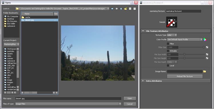
Figure 10-19 The blue sky of the desert image colors the reflections on the metal of the helmet.

c10f019.tif

To increase the realism of the reflections, you can add an ambient occlusion node to decrease the intensity of the reflections in the crevices of the model. Using ambient occlusion is discussed in Chapter 9. In this example, the mib_ambient_occlusion node is used as part of the helmet shader network:

1. Open the Attribute Editor of the mib_glossy_reflection node.
2. Click the checkered box next to Reflection Color. From the Create Render Node pop-up, select the Textures heading under mental ray in the list.
3. Click the mib_amb_occlusion node button on the right of the Create Render Nodes window.
4. Open the Attribute Editor for the mib_amb_occlusion node, and enter the following settings:
Samples: 32
Bright Color: Medium gray
Dark Color: Very dark gray (but not black)
Max Distance: 5
Turn on Reflective.
5. Create another test render of the scene. Now the reflections on the model look much more believable because the areas of the model within the crevices are not reflecting as much light as the areas that are fully exposed (see Figure 10-20). Again, if you are having trouble seeing these subtle changes in reflectivity, you can set the Diffuse attribute of the Cook-Torrance shader to black.

Figure 10-20 Adding an ambient occlusion node to control the reflectivity on the surface of the helmet helps to add realism to the render.

c10f020.tif
6. Save the scene as helmet_v04.ma.

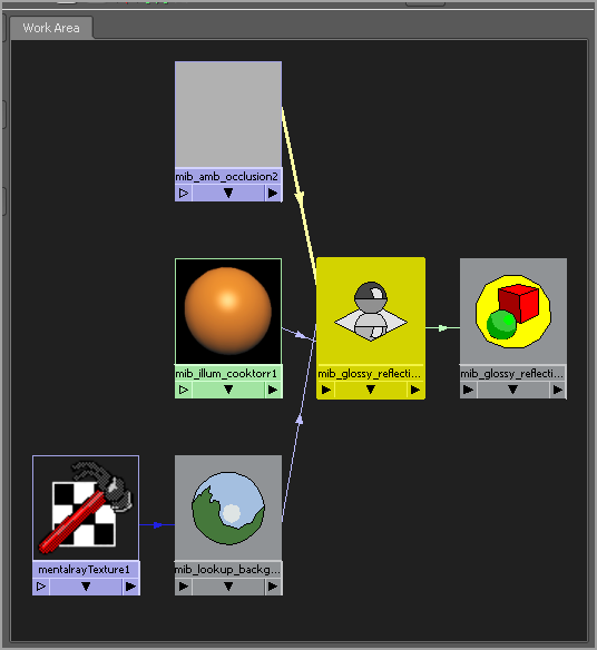
Figure 10-21 shows the shader network for this material.

Figure 10-21 The mental ray base shaders are connected to create a realistic painted-metal surface for the helmet.

c10f021.tif

This gives you an idea of how to work with the mental ray base materials. Of course, you can make many more complex connections between nodes to create even more realistic and interesting surface materials. Experimentation is a good way to learn which connections work best for any particular situation.

To see a version of the scene up to this point, open the helmet_v04.ma scene from the chapter10scenes folder at the book’s web page.

Car Paint Materials

Simulating the properties of car paint and colored metallic surfaces is made considerably easier thanks to the special car paint phenomenon and metallic paint mental ray materials.

In reality, car paint consists of several layers; together these layers combine to give the body of a car its special, sparkling quality. Car paint uses a base-color pigment, and the color of this pigment changes hue depending on the viewing angle. This color layer also has thousands of tiny flakes of metal suspended within it. When the sun reflects off these metallic flakes, you see a noticeable sparkling quality. Above these layers is a reflective clear coat, which is usually highly reflective (especially for new cars) and occasionally glossy. The clear coat itself is a perfect study in Fresnel reflections. As the surfaces of the car turn away from the viewing angle, the reflectivity of the surface increases.

The metallic paint material is similar to the car paint phenomenon material. In fact, you can re-create the car paint material by combining the mi_metallic_paint node with the mi_glossy_reflection node and the mi_bump_flakes node.

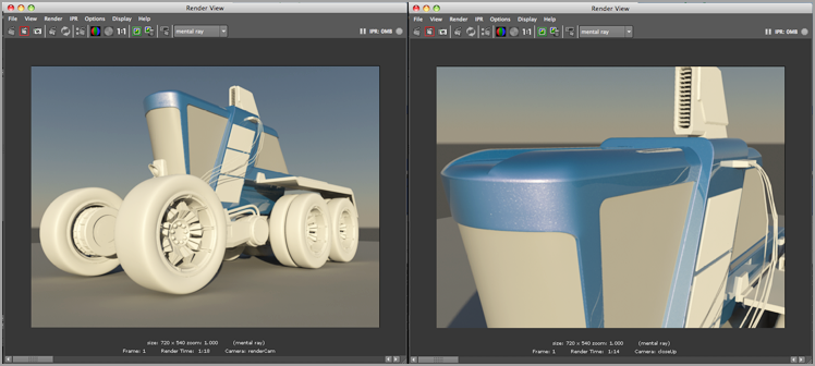
In this section, you’ll learn how to use the car paint material by applying it to the tractorDroid model created for this book by designer Anthony Honn.

1. Open the tractorDroid_v01.ma scene from the chapter10scenes folder at the book’s web page. This scene uses the Physical Sun and Sky network for lighting.

Physical Sun and Sky
When setting out to texture a model, sometimes we like to start by using the Physical Sun and Sky lighting model that was introduced in Chapter 9. As we develop the materials for the model, it’s helpful to see how they react to physically accurate lighting. This light setup uses Final Gathering, which can add a little extra time to the rendering because the image must go through two passes: one to calculate the Final Gathering and a second to render the image. All of this is explained in detail in Chapter 9.

2. Open the Hypershade window, and select the Materials heading in the mental ray section on the left side of the Hypershade window.
3. Click the mi_car_paint_phen_x shader button (see Figure 10-22).

Figure 10-22 The car paint materials are in the Materials section of the mental ray Nodes section in the Hypershade.

c10f022.tif

mental ray Extended Materials
The mental ray nodes that use the x suffix are more advanced (extended) versions of the original shader. Most of the advancements are in the back end; the interface and attributes of mi_car_paint_phen and mi_car_paint_phen_x are the same. It’s safe to use either version. You can upgrade the mi_car_paint_phen material by clicking the buttons in the Upgrade Shader section of the material’s Attribute Editor. The x_passes materials are meant to be used with render passes. For the most part, we use the materials with the x suffix and later upgrade the material if we decide we need to use render passes. Render passes are covered in Chapter 12.

4. The body of the tractor droid already has two shaders applied. In the Materials tab on the right side of Hypershade, right-click the body_shader icon, and choose Select Objects With Material; this will select all the polygons on the model that use this shader (see Figure 10-23).

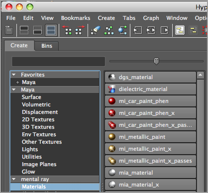
Figure 10-23 Use the Hypershade marking menu to select the parts of the model that use the body_shader material.

c10f023.tif
5. Right-click the mi_car_paint_phen_x shader created in step 3, and choose Assign Material To Selection (see Figure 10-24). Doing so applies the car paint material to the selected polygons. Parts of the tractor body should now appear red.

Figure 10-24 Use the Hypershade marking menu to assign the mi_car_paint_phen_x shader.

c10f024.tif
6. Open the Attribute Editor for the mi_car_paint_phen_x shader. Rename the shader carPaint (Figure 10-25).

Figure 10-25 The settings for the car paint shader
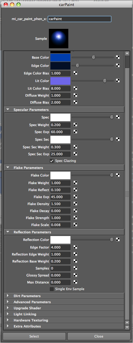
c10f025.tif

Diffuse Parameters

At the top of the attributes, you’ll find the Diffuse Parameters rollout. The settings here determine the color properties of the base pigment layer. As the color of this layer changes depending on the viewing angle, the various settings determine all the colors that contribute to this layer.

1. Set Base Color to dark navy blue; this is the main color of the base layer. If you wanted to add a texture map to apply decals to the car, you would use this channel.
2. Set Edge Color to a similar shade of blue, but lower the value so that it is almost black. The Edge Color is apparent on the edges that face away from the camera. Newer cars and sports cars benefit from a dark Edge Color.
Edge Color Bias sets the amount of spread seen in the Edge Color. Lower values (0.1 to 3) create a wider spread; higher values (4 to 10) create a narrower band of Edge Color.
3. Lit Color is the color seen in the surface areas that face the light source. Set this color to a bright purplish blue.
Lit Color Bias works on the same principle as Edge Color Bias. Lower values (above 0) create a wider spread in the Lit Color.
4. Diffuse Weight and Diffuse Bias set the overall strength of the Diffuse colors. Set Diffuse Bias to 2.
A lower Diffuse Bias value (0 to 1) flattens the color; higher values (1 to 2) increase intensity toward the lit areas.

Specular Parameters

The Specular Parameters settings define the look of the specular highlight on the surface. In this particular shader, these settings are separate from the Reflection Parameters settings. By adjusting the settings in Specular Parameters, you can make the car paint look brand-new or old and dull.

Here is how the settings work:

  • When rendered, the specular highlight has two components: a bright center highlight and a surrounding secondary highlight. Spec Weight and Spec Sec Weight are multipliers for the primary specular and secondary specular colors (respectively).
  • Spec Exp and Spec Sec Exp determine the tightness of the highlight; higher values (30 and greater) produce tighter highlights. Generally, Spec Sec Exp should be less than Spec Exp.
  • The Spec Glazing check box at the bottom of the Specular Parameters section adds a polished shiny quality to the highlight, which works well on new cars. Turn this feature off when you want to create the look of an older car with a duller finish.

For our next exercise, you can leave the specular parameters at their default settings.

Flake Parameters

The Flake Parameters settings are the most interesting components of the shader. These determine the look and intensity of the metallic flakes in the pigment layer of the car paint:

Flake Color Should usually be white for new cars.
Flake Weight A multiplier for Flake Color. Higher values intensify the look of the flakes; 1 is usually a good setting for most situations.
Flake Reflect Adds raytracing reflectivity to the flakes. This means that the flakes contribute to reflections of objects in the scene. For most situations, a value of 0.1 is sufficient.
Flake Exp The specular exponent for the flakes. Much like Spec Exp, higher values create a tighter highlight.
Flake Density Determines the number of flakes visible in the paint. The values range from 0.1 to 10. In many situations, a high value means that the individual flakes are harder to see.
Flake Decay Optimizes rendering times by setting a limit to the visibility of the flakes. Beyond the distance specified by this value, the flakes are no longer rendered, which can keep render times down and reduce render artifacts, especially if Flake Density is set to a high value.
Flake Strength Varies the orientation of the flakes in the paint. Setting this to 0 makes all the flakes parallel to the surface; a setting of 1 causes the flakes to be oriented randomly, making the flakes more reflective at different viewing angles.
Flake Scale Sets the size of the flakes. It’s important to understand that the size of the flakes is connected to the scale of the object. If you notice that the size of the flakes is different on one part of the car compared to the others, select the surface geometry and freeze the transformations so that the Scale X, Y, and Z values are all set to 1. This will correct the problem and ensure that the flakes are a consistent size across all the parts of the car.

For this exercise, use the following settings:

Flake Reflect: 0.1
Flake Density: 1.5
Flake Strength: 1
Flake Scale: 0.008

Reflection Parameters

The Reflection Parameters settings are similar to those for the reflection parameters on the glossy reflection material. The reflectivity of the surface is at its maximum when Reflection Color is set to white. When this option is set to black, reflections are turned off.

Edge Factor Determines the transition between the reflection strength at glancing angles and the reflection strength at facing angles.
Reflection Edge Weight and Reflection Base Weight Reflection Edge Weight sets the strength of reflectivity at glancing angles, and Reflection Base Weight sets the reflectivity at facing angles. Generally, the base weight should be lower than the edge weight to create a proper Fresnel reflection effect.
Samples Sets the sampling for glossy reflections. Unless you want to create blurry reflections, which are best used for older, duller cars, you can leave Samples at 0.
Glossy Spread Defines the glossiness of the reflections. Max Distance sets the point where reflection rays start sampling environment shaders and stop sampling the geometry in the scene.
Dirt Parameters The Dirt Parameters settings allow you to add a layer of dirt to the surface of the car. Dirt Weight specifies the visibility strength of the dirt. For best results, you can connect a painted texture map to Dirt Color if you want to add splashes of mud and grime.

Once you’ve familiarized yourself with the reflectivity settings, follow these steps:

1. Set Edge Factor to 4, and leave the other settings at their defaults (refer back to Figure 10-25).
2. In the Render View window, create a test render from the renderCam camera (see Figure 10-26).

Figure 10-26 The car paint material is applied to the body of the car and rendered with the Physical Sun and Sky lighting model.

c10f026.tif
3. Store the image in the render view, and create a second test render from the closeUp camera.
4. Save the scene as tractorDroid_v02.ma.

To see a finished version of the scene, open the tractorDroid_v02.ma file from the chapter10scenes folder at the book’s web page.

The mia Material

The mia material is the Swiss Army knife of mental ray shaders. It is a monolithic material, meaning that it has all the functionality needed for creating a variety of materials built into a single interface. You don’t need to connect additional shader nodes into a specific network to create glossy reflections, transparency, and the like.

mia stands for mental images architectural, and the shaders (mia_material, mia_material_x, mia_material_passes) and other lighting and lens shader nodes (mia_physicalsun, mia_portal, mia_exposure_simple, and so on) are all part of the mental images architectural library. The shaders in this library are primarily used for creating materials used in photorealistic architectural renderings; however, you can take advantage of the power of these materials to create almost anything you need.

The mia material has a large number of attributes that at first can be overwhelming. However, presets are available for the material. You can quickly define the look you need for any given surface by applying a preset. Then you can tune specific attributes of the material to get the look you need.

Using the mia Material Presets

The presets that come with the mia material are the easiest way to establish the initial look of a material. Presets can also be blended to create novel materials. Furthermore, once you create something you like, you can save your own presets for future use in other projects. You’ll work on defining materials for the space helmet. Just like the example in the previous section, this version of the scene uses the mia_physicalsunsky lighting network and Final Gathering to light the scene.

1. Open the helmet_v05.ma scene from the chapter10scenes folder at the book’s web page. The surfaces in the model have been grouped by material type to make it easier to apply shaders.
2. Open the Hypershade window, and select Materials under the mental ray section of the list on the left of the editor.
3. Click the mia_material_x button to create a material, and name it metalShader.
4. In the Outliner, select the helmetMetalSurfaces group, and apply the metalShader material to this group (right-click the material in the Hypershade, and choose Assign Material To Selection).
5. Open the Attribute Editor for the metalShader.
6. Click the Presets button in the upper right, and choose Copper ⇒ Replace.
7. Open the Render View window, and create a render from the renderCam camera. It really looks like copper. Save the render in the Render View.
8. The material could use a little tweaking to make it look less like a kitchen pot. Click the Presets button again, and choose SatinedMetal ⇒ Blend 50%. This will add some anisotropy to the highlights on the helmet.
9. In the Attribute Editor, scroll to the Diffuse rollout at the top.
10. Set Color to a medium grayish-blue (the color should be fairly unsaturated; otherwise, the helmet will look very disco!).
11. Just below the Diffuse rollout, in the Reflection section, set Color to a light blue, and turn on Metal Material—this adds a bluish tint to the reflections.
12. Create another test render, and compare it with the previous render (see Figure 10-27).

You can tweak many of the settings to create your own custom metal, and already it looks pretty good. Like with the other materials in this chapter, the Glossiness setting adds blur to the reflections. Turning on Highlights Only creates a more plastic-like material—with this option activated, the Reflection settings apply only to specular highlights.

Next you can add chrome to the helmet:

1. Create a new mia_material_x shader, and name it chromeShader.
2. Select the chromeParts group in the Outliner, and apply the chromeShader to the group.
3. Open the Attribute Editor for the chromeShader material.
4. Click the Presets button, and apply the Chrome preset to the shader.

Figure 10-27 The mia material comes with a number of presets that can be blended together to create novel materials. For example, blending the Copper and SatinedMetal presets creates a convincing metallic surface.

c10f027.tif
5. Create another mia_material_x shader, and name it rubberShader. Apply this shader to the rubberParts group. Use the Presets button to apply the Rubber preset.
6. Create another test render, and compare it to the previous renders.

Add Bumps to the Rubber Shader

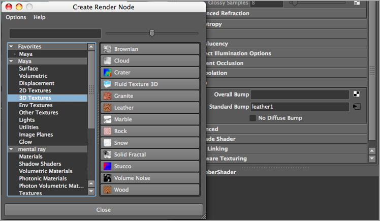
The rubber shader can use a little tweaking. A slight bumpiness can increase the realism. The mia_material has two slots for bump textures under the Bump rollout; they’re labeled Standard Bump and Overall Bump. Standard Bump works much like the bump channel on a standard Maya shader (Blinn, Lambert, Phong, and so on). Overall Bump is used primarily for the special mia_roundcorners texture node, which is explained in the next section.

When using a texture to create a bump effect, connect the texture to the Standard Bump slot, as demonstrated in this exercise:

1. Scroll down in the Attribute Editor for the rubber shader, and click the checkered box next to Standard Bump.
2. In the Create Render Nodes pop-up, select the 3D Textures heading under Maya in the list on the left, and click Leather to create a Leather texture node (see Figure 10-28).

Figure 10-28 The Leather texture is added as a bump to the rubber mia material.

c10f028.tif
3. Open the Attribute Editor for the leather1 node. (It should open automatically when you create the node.) Use the following settings:
Cell Color: Light gray
Crease Color: Dark gray
Cell Size: 0.074
4. In the Hypershade work area, select the rubber shader, and choose Graph ⇒ Input And Output Connections from the Hypershade menu.
5. Select the bump3d1 node, and open its Attribute Editor. Set the Bump Depth value to 0.1. This value makes the bump effect less prominent and creates a more realistic look for the rubber. Bump maps are covered in greater detail in Chapter 11.
6. Create a test render of the helmet using the closeUp camera (see Figure 10-29).

You’ll notice that in the Bump rollout there is a No Diffuse Bump check box. When a texture is connected to the Standard Bump field and No Diffuse Bump is activated, the bump appears only in the specular and reflective parts of the material, which can be useful for creating the look of a lacquered surface.

Figure 10-29 The bump adds realism to the rubber parts of the helmet.

c10f029.tif

Create Beveled Edges Using mia_roundcorners

A very slight edge bevel on the corners of the model can improve the realism of the model. (Sharp edges on a surface are often a telltale sign that the object is computer generated.) Usually, this bevel is created in the geometry, which can add a lot of extra vertices and polygons. The mia_roundcorners texture adds a slight bevel to the edges of a surface that appears only in the render, which means that you do not need to create beveled edges directly in the geometry.

The mia_roundcorners texture is attached to the Overall Bump channel of the mia_material. The reason the mia_material has two bump slots is so that you can apply the roundcorners texture to the Overall Bump shader and another texture to the Standard Bump shader to create a separate bumpy effect.

Let’s take a look at the roundcorners texture in action by applying it to the chrome material:

1. First create a render in the Render View window from the closeUp camera, and store the image so that you can compare it after the changes are made to the shader.
2. In the Hypershade, select the chromeShader and open its Attribute Editor.
3. Scroll down to the Bump section, and click the checkered box to the right of Overall Bump.
4. In the Create Render Nodes pop-up, select the Textures heading from the list of mental ray nodes on the left, and click the mia_roundcorners button on the right side to create this node.
5. In the Attribute Editor for the mia_roundcorners1 node, set Radius to 0.1.
6. Create another test render, and compare it to the previous renders. You’ll see that the chrome trim around the helmet has a slight roundness to it, making it look a little more believable.
7. Try adding a mia_roundcorners node to the metalShader, and see how it affects the render. Use a Radius value of 0.05 (see the right image of Figure 10-30).

Figure 10-30 Adding the mia_roundcorners texture to the chromeShader’s Overall Bump channel creates a slight beveled edge, as is demonstrated by the right render. Compare the edges to the left image, which does not have this beveled effect applied.

c10f030.eps

To see a version of the scene, open the helmet_v06.ma scene from the chapter10scenes folder at the book’s web page.

Creating Thick and Thin Glass and Plastic

Another feature of the mia_material shader is the ability to simulate thickness and thinness in the material itself without creating extra geometry. This can be very useful, especially for glass surfaces.

1. Continue with the scene from the previous section, or open the helmet_v06.ma file from the chapter10scenes folder at the book’s web page.
2. In the Hypershade, create two new mia_material_x nodes. Name one thinGlass and the other thickGlass.
3. Apply the thinGlass shader to the glassShield object in the Outliner.
4. Apply the thickGlass material to the lampShields group in the Outliner.
5. In the Attribute Editor for the thinGlass material, use the Preset button to apply the glassThin preset.
6. In the Attribute Editor for the thickGlass shader, apply the glassThick preset.
7. Create another test render from the renderCam camera.

The lamps at the top of the helmet have a chrome reflector behind the thick glass, which adds to the reflectivity of the material. The settings to control thickness are found under the Advanced Refractions controls. Along with the standard Index Of Refraction setting, there is an option for making the material either thin-walled or solid. You also have the option of choosing between a transparent shadow and a refractive caustic that is built into the material (the caustics render when caustic photons are enabled and the light source emits caustic photons; for more information on caustics, consult Chapter 9).

1. Open the Hypershade window, and create another mia_material_x node. Name this one plastic. Apply this shader to the plasticParts group in the Outliner.
2. Open the Attribute Editor for the plastic shader, and apply the translucentPlasticFilmLightBlur preset.
3. Create another test render.
This preset creates very translucent plastic using glossy refractions. In this situation, it seems a little too transparent. Use the following settings to make the plastic look more substantial:
a. In the Diffuse section, set Color to a dim pale blue.
b. In the Reflection section, set Color to a dark gray, and set Glossiness to 0.35.
c. In the Refraction section, set Color to a dark blue and Glossiness to 0.52.
d. Scroll down to the Ambient Occlusion section, and activate Ambient Occlusion.
e. Set Ambient Light Color to a light gray.
4. Create another test render (see Figure 10-31).

Figure 10-31 Apply the glass and plastic presets to parts of the helmet.

c10f031.tif
5. Save the scene as helmet_v07.ma.

To see a finished version of the scene, open the helmet_v07.ma scene from the chapter10scenes folder at the book’s web page.

Other mia Material Attributes

The mia_material has a lot of settings that can take some practice to master. It’s a good idea to take a look at the settings used for each preset and note how they affect the rendered image. Over time, you’ll pick up some good tricks using the presets as a starting point for creating your own shaders. The following sections give a little background on how some of the other settings work.

Built-in Ambient Occlusion

The Ambient Occlusion option on the material acts as a multiplier for existing ambient occlusion created by the indirect lighting (Final Gathering/Global Illumination). The Use Detail Distance option in the Ambient Occlusion section can be used to enhance fine detailing when set to On. When Use Detail Distance is set to With Color Bleed, the ambient occlusion built into the mia_material factors the reflected colors from surrounding objects into the calculation.
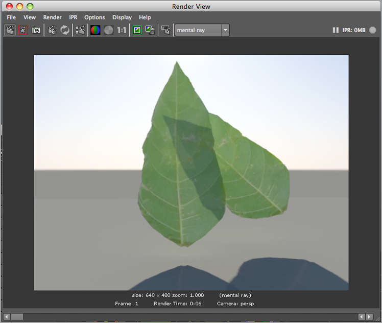
Translucency

The Translucency setting is useful for simulating thin objects, such as paper, that allow some amount of light to pass through them. This option works only when the material has some amount of transparency. The Translucency Weight setting determines how much of the Transparency setting is used for transparency and how much is used for translucency. So if Transparency is 1 (and the transparency color is white) and Translucency Weight is 0, the object is fully transparent (see Figure 10-32, left). When Translucency Weight is at 0.5, the material splits the Transparency value between transparency and translucency (Figure 10-32, center). When Translucency Weight is set to 1, the object is fully translucent (Figure 10-32, right).

Notice that you can also create translucent objects by experimenting with the glossiness in the Refraction settings. This can be used with or without activating the Use Translucency option. If you find that the translucency setting does not seem to work or make any difference in the shading, try reversing the normals on your geometry (in the Polygons menu set, choose Normals ⇒ Reverse). The mia materials have a wide variety of uses beyond metal and plastic. The materials offer an excellent opportunity for exploration. For more detailed descriptions of the settings, read the mental ray for Maya Architectural Guide in the Maya documentation.

Figure 10-32 Three planes with varying degrees of translucency applied

c10f032.tif

Using the mia_material to Shade Organic Objects
The many settings of the mia_material can be used to create material properties well beyond what is listed in the Presets menu. In fact, the mia_material is by far our favorite shader available in Maya because of its versatility. The Translucency attributes make it ideal for shading things like leaves in a close-up, insect wings, and clothing. We’ve even used the material to create the look of flakes of skin as seen on a microscopic scale.
You can create these effects by mapping file textures to various channels of the mia_material. Mapping file textures is covered in depth in Chapter 11, but this example should be simple enough to follow even if you have not worked with texture maps very much.
The mia_shader has an advanced attribute called Cutout Opacity. This is like a second transparency channel that is used to map a texture to define the silhouette of an object. Here’s how you can use this channel:
1. Open the leaves_v01.ma scene from the chapter10scenes folder at the book’s web page.
2. In the Hypershade editor, create a new mia_material_x shader.
3. Apply this shader to the leaf1 and leaf2 objects in the scene.
4. Create a new file texture node (select 2D Textures from under the Maya heading in the list on the left), and click the File button.
5. Open the Attribute Editor for the file1 node.
6. Click the Image Name field. Browse your computer, and find the leaf.tif file located in the chapter10sourceimages folder.
7. MMB-drag the file1 node from the Hypershade to the color swatch in the Diffuse rollout of the mia_material_x1 node’s Attribute Editor.
8. Repeat step 7, but this time connect the file1 node to the Color swatch in the Refraction node. This will use the file1 image, which is a picture of a leaf, to color the transparency of the leaf objects.
9. In the Reflection rollout, set Reflectivity to 0.18 and Glossiness to 0.2.
10. In the Refraction rollout, set Transparency to 0.15.
11. In the Translucency rollout, turn on Use Translucency. Set Color to a light gray and Weight to 0.8.
12. Create a test render.
These are some nice-looking translucent leaves, but there is an ugly black box appearing around the leaf image in the texture. This is where Cutout Opacity is useful. You can easily use this channel to create the edges of the leaves based on the alpha channel stored in the original leaf.tif file.
13. Expand the Advanced rollout toward the bottom of the mia_material_x1 shader’s Attribute Editor.
14. MMB-drag the file1 node from the Hypershade window onto the Cutout Opacity slider. This will automatically connect the alpha channel of the file1 texture to the Cutout Opacity setting.
15. Create another test render. Voilà! Translucent leaves!
c10uf003.tif
This technique is useful because the shader can be applied to very simple geometry. The planes used for the leaves can be turned into nCloth objects and have dynamic forces create their movement. (nCloth and Dynamics are covered in Chapter 14, “Dynamic Effects,” and Chapter 15, “Fur, Hair, and Clothing.”)
There are several things you may need to remember to determine whether this technique is working in your own scenes:
  • Make sure the normals of your polygon objects are facing in the correct direction.
  • Make sure the file texture you use for Cutout Opacity has an alpha channel.
  • Make sure that the Transparency setting is above 0 in order for the translucency to work.
You may notice that the texture was connected to the refraction color and not the translucency color. This is so that the shadows cast by the leaves are semitransparent. You can map a texture to the translucency color, but your shadows may appear black.
Another useful setting is the Additional Color channel in the Advanced rollout. This can be used to create incandescent effects similar to the incandescence channel on standard Maya shaders (Blinn, Phong, Lambert, and so on).

Controlling Exposure with Tone Mapping

Tone mapping refers to a process in which color values are remapped to fit within a given range. Computer monitors lack the ability to display the entire range of values created by physically accurate lights and shaders. This becomes apparent when using HDRI lighting, mia materials, and the physical light shader. Using tone mapping, you can correct the values to make the image look visually pleasing when displayed on a computer monitor.

Lens shaders are applied to rendering cameras in a scene. Most often, they are used for color and exposure correction. You’ve already been using the mia_physicalsky lens shader, which is created automatically when you create the Physical Sun and Sky network using the controls in the Indirect Lighting section of the Render Settings window.


Adding Cameras to the Physical Sun and Sky Network
When you add a new camera to a scene that already has the Physical Sun and Sky network, you may find that the images rendered with this camera look all wrong. To fix this, you need to add the camera to the Physical Sun and Sky network. To do this, follow these steps:
1. Select the sunDirection node in the Outliner.
2. Open its Attribute Editor, and switch to the mia_physicalsky tab.
3. Click Update Camera Connections at the bottom of the Attribute Editor. Doing so ensures that the correct lens shaders are applied to the camera.
The Physical Sun and Sky network is discussed in detail in Chapter 9.

The mia_exposure_photographic and mia_exposure_simple shaders are used to correct exposure levels when rendering with physically based lights and shaders. The mia_exposure_photographic lens shader has a lot of photography-based controls that can help you correct the exposure of an image. The mia_exposure_simple lens shader is meant to accomplish the same task; however, it has fewer controls and is easier to set up and use. In this exercise, you’ll use the mia_exposure_simple lens shader to fix problems in a render.

The scene you’ll use is the space helmet scene. This version of the scene uses the same mia_materials as the previous section. In the previous section, the problems with the exposure were not noticeable because lens shaders were already applied to all the cameras when the Physical Sun and Sky network was created. In this section, you’ll learn how to apply the lens shader manually:

1. Open the helmet_v08.ma scene from the chapter10scenes folder on the book’s web page. Currently this scene has no lighting. All the materials on the helmet are the same mia materials described in the previous section.
2. Open the Render Settings window, and switch to the Indirect Lighting tab.
3. Click the Create button next to Image Based Lighting. (Image Based Lighting is covered in detail in Chapter 9.)
4. In the Attribute Editor for the mentalrayIbl1 node, click the folder next to Image Name.
5. You’ll need a high-dynamic range (HDR) image to use for the mentalrayIbl node. You can download a number of these images free of charge from Paul Debevec’s website at http://ict.debevec.org/~debevec/Probes.
a. Follow the link in the text to download the all_probes.zip file.
b. Unzip these files, and place them in the sourceimages folder of your current project.
6. Choose the building_probe.hdr image from the all_probes folder.
7. Set Mapping to Angular.
8. In the Render Stats section, turn off Primary Visibility so that the IBL sphere is not visible in the render.
9. Enable Final Gathering on the Indirect Lighting tab of the Render View window, and set Accuracy to 200.
10. Create a test render in the Render View window using the renderCam camera, and store the image in the Render View window.
The rendered image looks underexposed; the dark parts are very dark (see the left image in Figure 10-33).
11. In the Outliner, select the renderCam camera and open its Attribute Editor.
12. Expand the mental ray section, and click the checkered box to the right of Lens Shader.
13. In the Create Render Nodes window, select the Lenses heading in the mental ray section.
14. Click the mia_exposure_simple button.
This applies the mia_exposure_simple lens shader to the rendering camera. You need to remember to apply this shader to any of the cameras you’ll use for rendering the scene.

Figure 10-33 The image on the left appears underexposed; adding a lens shader to control exposure fixes the problem, as shown in the image on the right.

c10f033.tif
15. Create another test render from the renderCam camera. You’ll see a big improvement in the image using the default settings of the mia_exposure_simple lens shader (see the right image in Figure 10-33).
16. Save the scene as helmet_v09.ma.

To see a finished version of the scene, open the helmet_v09.ma scene from the chapter10scenes folder at the book’s web page.

The following is a brief description of the mia_exposure_simple shader’s attributes:

Pedestal Adds lightness to the black areas of the image; a negative value will “crush the blacks” by adding contrast to the image.
Gain Increases the brightness of the lighter areas in the image.
Knee Value Sets the point where overly bright values (values that go beyond the 0–1 range) are brought down within the normal range.
Compression Setting Applies compression to the overly bright values as defined by the Knee setting.
Gamma Applies the overall color correction to the image so that it appears correct on the computer monitor. A typical value for Windows displays is 2.2. It’s important to make sure that, if you set the Gamma value in the lens shader, additional gamma correction does not take place in the rendering and compositing pipeline.

For a more in-depth discussion of tone mapping, consult the mental ray for Maya Architectural Guide included in the Maya documentation.

Rendering Contours

mental ray has a special contour-rendering mode that enables you to render outlines of 3D objects. This is a great feature for non-photorealistic rendering. You can use it to make your 3D animations appear like drawings or futuristic computer displays. The end title sequence of the film Iron Man is a great example of this style of rendering.

Rendering contours is easy, but it requires activating settings in several places. Furthermore, it is not supported by Unified Sampling. The Legacy Sampling mode must be used. The following steps take you through the process of rendering with contours:

1. Open the tractorDroidContour_v01.ma scene from the chapter10scenes folder at the book’s web page. This scene shows the vehicle modeled by Anthony Honn. A standard Maya Lambert material is applied to the tractor.
2. Open the Render Settings window, and under the Quality tab, change Sampling Mode to Legacy Sampling Mode.
3. Select the Features tab. Expand the Contours section, and click Enable Contour Rendering. This makes contour rendering possible, but you won’t see any results until you activate a few more options.
4. Expand the Draw By Property Difference section. These settings define how the contours will be drawn. One of these options must be activated, or contour rendering will not take place. Click Between Different Instances. This means that lines will be drawn around each piece of geometry in the scene (see Figure 10-34).

Figure 10-34 To render contour lines, you must select Enable Contour Rendering and choose a Draw By Property Difference option.

c10f034.tif
5. Open the Hypershade window, select the whiteLambert material, and graph its input and output connections.
6. In the work area of the Hypershade, select the whiteLambert4SG node that is attached to the whiteLambert shader and open its Attribute Editor. Switch to the whiteLambert4SG tab.
7. In the Contours section of the mental ray rollout in the Attribute Editor, select the Enable Contour Rendering option. Set Color to red (see Figure 10-35).

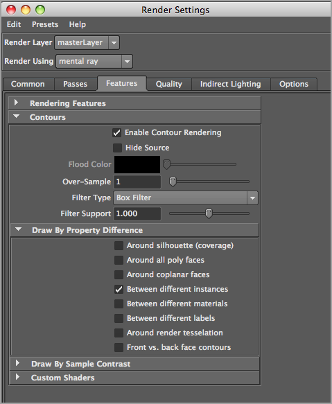
Figure 10-35 Contour Rendering also needs to be enabled in the shader’s shading group node settings.

c10f035.tif
8. Create a test render in the Render View window from the renderCam camera. The contours are added after the scene renders, on top of the shaded view of the geometry.
9. Open the Render Settings window.
10. In the Features tab, in the Contours section, activate Hide Source, and set Flood Color to a dark blue.
11. Create another test render (see Figure 10-36).

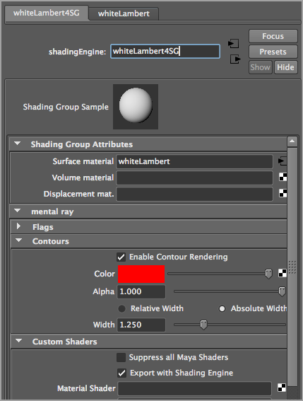
Figure 10-36 Contour rendering creates lines on top of the rendered surface. In the right image, the source has been hidden, so only the lines render.

c10f036.tif

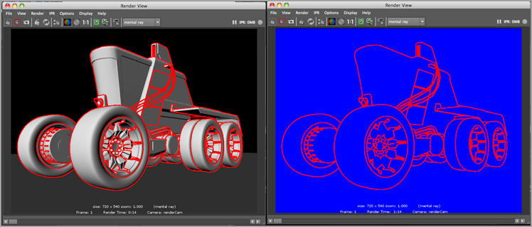
This time the original geometry is hidden, and only the contours are rendered. Flood Color determines the background color when Hide Source is activated. Oversampling sets the quality and antialiasing of the contour lines. To see a finished version of the scene, open the tractorDroidContour_v02.ma scene from the chapter10scenes folder at the book’s web page.

You can adjust the width of the contours using the controls in the Contours section of the shading group. Absolute Width ensures that the contours are the same width; Relative Width makes the width of the contours relative to the size of the rendered image.

Since each shading group node has its own contour settings, you can create lines of differing thickness and color for all the parts of an object. Just apply different materials to the different parts, and adjust the settings in each material’s shading group node accordingly.

Experiment using different settings in the Draw By Property Difference section of the Render Settings window. More complex contour effects can be created by plugging one of the contour shaders available in the Create mental ray Node section of the Hypershade into the Contour Shader slot under the Custom Shaders section of the shading group node.

The Bottom Line

Understand shading concepts Light rays are reflected, absorbed by, or transmitted through a surface. A rough surface diffuses the reflection of light by bouncing light rays in nearly random directions. Specular reflections occur on smooth surfaces; the angle at which rays bounce off a smooth surface is equivalent to the angle at which they strike the surface. Refraction occurs when light rays are bent as they are transmitted through the surface. A specular highlight is the reflection of a light source on a surface. In CG rendering, this effect is often controlled separately from reflection; in the real world, specular reflection and highlights are intrinsically related.
Master It Make a standard Blinn shader appear like glass refracting light in the jellybeans_v01.ma scene in the chapter10scenes folder on the book’s web page.
Apply reflection and refraction blur Reflection and Refraction Blur are special mental ray options available on many standard Maya shading nodes. You can use these settings to create glossy reflections when rendering standard Maya shading nodes with mental ray.
Master It Create the look of translucent plastic using a standard Maya Blinn shader.
Use basic mental ray shaders The DGS and Dielectric shaders offer numerous options for creating realistic reflections and transparency. The mib (mental images base) shader library has a number of shaders that can be combined to create realistic materials.
Master It Create a realistic CD surface using the mib shaders.
Apply the car paint shader Car paint consists of several layers, which creates the special quality seen in the reflections on car paint. The mi_carpaint_phen_x shader can realistically simulate the interaction of light on the surface of a car model. The diffuse, reflection, and metallic-flakes layers all work together to create a convincing render.
Master It Design a shader for a new and an old car finish.
Use the mia materials The mia materials and nodes can be used together to create realistic materials that are always physically accurate. The mia materials come with a number of presets that can be used as a starting point for your own materials.
Master It Create a realistic polished-wood material.
Render contours mental ray has the ability to render contours of your models to create a cartoon drawing look for your animations. Rendering contours requires that options in the Render Settings window and in the shading group for the object are activated.
Master It Render the spacesuit helmet using contours.
..................Content has been hidden....................

You can't read the all page of ebook, please click here login for view all page.
Reset