Chapter 14
Dynamic Effects
The nCloth system in the Autodesk® Maya® software was originally designed to make dynamic cloth simulation for characters easier to create and animate. The Nucleus dynamics solver, which you learned about in Chapter 13, “Introducing nParticles,” is at the heart of nCloth simulations. (The n in nCloth stands for “nucleus.”) nCloth has evolved into a dynamic system that goes well beyond simply simulating clothing. Creative use of nCloth in combination with nParticles yields nearly limitless possibilities for interesting effects, as you’ll see when you go through the exercises in this chapter.
In this chapter, you’ll delve deeper into Maya dynamics to understand how the various dynamic systems, such as nCloth, nParticles, and rigid bodies, can be used together to create spectacular effects. You’ll also use particle expressions to control the motion of particle instances.
In this chapter, you will learn to:
- Use nCloth
- Combine nCloth and nParticles
- Use Maya rigid body dynamics
- Use nParticles to drive instanced geometry
- Create nParticle expressions
Creating nCloth Objects
Typically, nCloth is used to make polygon geometry behave like clothing, but nCloth can be used to simulate the behavior of a wide variety of materials. Everything from concrete to water balloons can be achieved by adjusting the attributes of the nCloth object. nCloth uses the same dynamic system as nParticles and applies it to the vertices of a piece of geometry. An nCloth object is simply a polygon object that has had its vertices converted to nParticles. A system of virtual springs connects the nParticles and helps maintain the shape of nCloth objects. nCloth objects automatically collide with other nDynamic systems (such as nParticles and nRigids) that are connected to the same Nucleus solver, and an nCloth object collides with itself.
In this section, you’ll see how to get up and running fast with nCloth using the presets that ship with Maya as well as get some background on how the Nucleus solver works. The examples in this chapter illustrate a few of the ways nCloth and nParticles can be used together to create interesting effects. These examples are only the beginning; there are so many possible applications and uses for nCloth that a single chapter barely scratches the surface. The goal of this chapter is to give you a starting place so that you feel comfortable designing your own unique effects. Chapter 15, “Fur, Hair, and Clothing,” demonstrates techniques for using nCloth to make clothing for an animated character.
Making a Polygon Mesh Dynamic
Any polygon mesh you model in Maya can be converted into a dynamic nCloth object (also known as an nDynamic object); there’s nothing special about the way the polygon object needs to be prepared. The only restriction is that only polygon objects can be used. NURBS and subdivision surfaces can’t be converted to nCloth.
There are essentially two types of nCloth objects: active and passive. Active nCloth objects are the ones that behave like cloth. They are the soft, squishy, or bouncy objects. Passive nCloth objects are solid pieces of geometry that react with active objects. For example, to simulate a tablecloth sliding off a table, the tablecloth would be the active nCloth object, and the table would be the passive nCloth object. The table prevents the tablecloth from falling in space. You can animate a passive object, and the active object will react to the animation. Thus you can keyframe the table tilting, and the tablecloth will slide off the table based on its dynamic settings.
The first exercise in this chapter shows you how to create the effect of a dividing cell using two nCloth objects:
2. Switch to the nDynamics menu set. Select both objects, and choose nMesh ⇒ Create nCloth. In the Outliner, you’ll see that two nCloth nodes have been added.
3. Switch to the wireframe mode, and select nCloth1. One of the cell halves turns purple, indicating the nCloth node is an input connection to that particular piece of geometry.
4. Rename the nCloth1 and nCloth2 nodes
cellLeftCloth and
cellRightCloth according to which piece of geometry they are connected to (see
Figure 14-1).
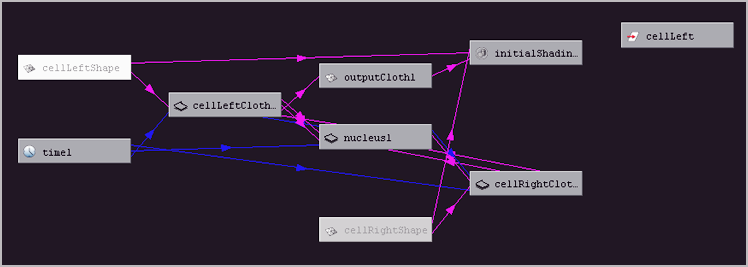
5. Set the timeline to 400 frames, and play the scene. You’ll see that both pieces of geometry fall in space. This is because Gravity is turned on by default in the Nucleus solver. When you create an nCloth object or any nCloth dynamic system (nParticles, nRigids), several additional nodes are created and connected. You can see this when you graph the cellLeftShape on the Hypergraph, as shown in
Figure 14-2.
Each nCloth object consists of the original geometry, the nCloth node, and the Nucleus solver. By default, any additional nDynamic objects you create are attached to the same Nucleus solver. Additional nodes include the original cellLeftShape node, which is connected as the inputMesh to the cellLeftClothShape node. This determines the original starting shape of the nCloth object.
6. Select the cellLeftCloth node, and open the Attribute Editor.
7. Switch to the cellLeftClothShape tab, as shown in
Figure 14-3. This node was originally named nCloth1. The tabs found in the Attribute Editor include the following:
cellLeftCloth This tab contains the settings for the nCloth1 transform node. Most of the time you won’t have a reason to change these settings.
cellLeftClothShape This tab contains the settings that control the dynamics of the nCloth object. There are a lot of settings on this tab, and this is where you will spend most of your time adjusting the settings for this particular nCloth object.
nucleus1 This tab contains all the global settings for the Nucleus solver. These include the overall solver quality settings but also the Gravity and Air Density settings. If you select the cellRightCloth node in the Outliner, you’ll notice that it also has a nucleus1 tab. In fact, this is the same node as attached to the cellLeftCloth object.
It’s possible to create different Nucleus solvers for different nDynamic objects, but unless the nDynamic objects are connected to the same Nucleus solver, they will not directly interact.
Name Your nCloth Nodes
Because the nCloth objects are connected to the same Nucleus solver, when you open the Attribute Editor for the nucleus node, you’ll see tabs for each node that are connected to the solver. To reduce confusion over which nCloth object is being edited, always give each nCloth node a descriptive name as soon as the node is created.
8. Choose the cellLeftClothShape tab. Under the Dynamic Properties section, change Input Motion Drag to 1.0.
Input Motion Drag controls how much the nCloth object follows its input mesh. Increasing it to 1.0 causes the simulated motion of the nCloth hemisphere to be blended with its stationary input mesh. By default, the input mesh or, in this case, the cellLeftShape node, is set to Intermediate Object under its Object Display settings. You can toggle its visibility by unchecking Intermediate Object or by choosing nMesh ⇒ Display Input Mesh.
9. Choose the cellRightClothShape tab. Change its Input Motion Drag to 1.0 as well.
When you rewind and play the scene, the cells slowly descend under the influence of gravity and their input meshes.
Applying nCloth Presets
The concept behind this particular example is that both halves of the cell together form a single circular spherical shape. To make the cells separate, you’ll adjust the nDynamic settings so that each half of the cell inflates and pushes against the other half, moving them in opposite directions. Creating the correct settings to achieve this action can be daunting simply because there is a bewildering array of available settings on each nCloth shape node. To help you get started, Maya includes a number of presets that can act templates. You can apply a preset to the nCloth objects and then adjust a few settings until you get the effect you want.
1. Continue with the scene from the previous section.
Maya Presets
You can create a preset and save it for any Maya node. For instance, you can change the settings on the nucleus1 node to simulate dynamic interactions on the moon and then save those settings as a preset named moonGravity. This preset will be available for any Maya session. Some nodes, such as nCloth and fur nodes, have presets already built in when you start Maya. These presets are created by Autodesk and other Maya users and can be shared between users. You’ll often find new presets available on the Autodesk Area website (
http://area.autodesk.com).
To apply a preset to more than one object, select all the objects, select the preset from the list, and choose Replace All Selected.
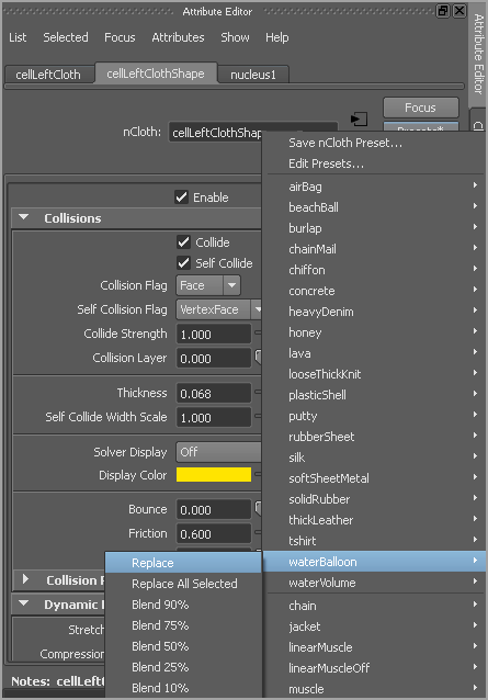
2. Select the cellLeftCloth node, and open the Attribute Editor to the cellLeftClothShape node.
3. At the top of the editor, click and hold the Presets button in the upper right. The asterisk by the button label means that there are saved presets available for use.
4. From the list of presets, scroll down to find the waterBalloon preset. A small pop-up appears; from this pop-up, choose Replace (see
Figure 14-4). You’ll see the settings in the Attribute Editor change, indicating the preset has been loaded.
5. Repeat steps 2 through 4 for the cellRightCloth node.
6. Rewind and play the animation. Immediately, you have a decent cell division.
Overlapping nCloth Objects
Initially it might seem like a good idea to have two overlapping nCloth objects that push out from the center. However, if the geometry of the two nCloth objects overlaps, it can confuse the Nucleus solver and make it harder to achieve a predictable result.
The next task is to create a more realistic behavior by adjusting the setting on the nCloth objects:
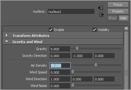
1. Switch to the nucleus1 tab, and set Air Density to
35 (see
Figure 14-5). This makes the cells look like they are in a thick medium, such as water.
2. You can blend settings from other presets together to create your own unique look. Select cellLeftCloth and, in its shape node tab, click and hold the Presets button in the upper right.
3. Choose Honey ⇒ Blend 10%. Do the same for the cellRightCloth.
4. Play the animation. The two cells separate more slowly.
5. You can save these settings as your own preset so that it will be available in other Maya sessions. From the Presets menu, choose Save nCloth Preset. In the dialog box, name the preset
cell (see
Figure 14-6).
6. Save the scene as cellDivide_v02.ma.
Saving Maya Presets
When you save a Maya preset, it is stored in a subfolder of maya2011presetsattrPresets. Your custom nCloth presets will appear in the nCloth subfolder as a MEL script file. You can save to this folder nCloth presets created by other users, and they will appear in the Presets list. If you save a preset using the same name as an existing preset, Maya will ask you if you want to overwrite the existing preset.
Making Surfaces Sticky
At this point, you can start to adjust some of the settings on the nCloth tabs to create a more interesting effect. To make the cells stick together as they divide, you can increase the Stickiness attribute:
1. Continue with the scene from the previous section, or open the cellDivide_v02.ma scene from the chapter14scenes folder at the book’s web page.
2. Select the cellLeftCloth node, and open the Attribute Editor to its shape node tab.
3. Expand the Collisions rollout, and set Stickiness to
1 (see
Figure 14-7). Do the same for the cellRight object.
Notice that many of the settings in the Collision rollout are the same as the nParticle Collision settings. For a more detailed discussion of how nucleus collisions work, consult Chapter 13.
4. Play the animation; the cells remain stuck as they inflate. By adjusting the strength of the Stickiness attribute, you can tune the effect so that the cells eventually come apart. Shift+click both the cellLeftCloth and cellRightCloth nodes in the Outliner. Open the Channel Box, and, with both nodes selected, set Stickiness to 0.4.
Edit Multiple Objects Using the Channel Box
By using the Channel Box, you can set the value for the same attribute on multiple objects at the same time. This can’t be done using the Attribute Editor.
5. We will manually move the right cell away from the left cell to get them to separate. To do so, it is best to turn off the Nucleus solver to prevent it from solving. Select nucleus1, and open its Attribute Editor.
6. Turn off Enable, effectively stopping the cells from being simulated.
7. Select cellRight, and keyframe its position at frame 10 for its translation and rotation.
8. Move to frame 100 on the timeline, and change the following attributes:
Translate Y: 7.0
Translate Z: -8.0
Rotate X: -50
You will not see the geometry move unless you display the cell’s input mesh.
9. Return to frame 1, and enable the Nucleus solver. Play the simulation to see the results (see
Figure 14-8).
10. Save the nCloth settings as stickyCell. Save the scene as cellDivide_v03.ma.
Create Playblasts Often
It’s difficult to gauge how the dynamics in the scene work using just the playback in Maya. You may want to create a playblast of the scene after you make adjustments to the dynamics so that you can see the effectiveness of your changes. For more information on creating playblasts, consult Chapter 5, “Animation Techniques.”
Creating nConstraints
nConstraints can be used to attach nCloth objects together. The constraints themselves can be broken depending on how much force is applied. In this example, nConstraints will be used as an alternative technique to the Stickiness attribute. There are some unique properties of nConstraints that can allow for more creativity in this effect.
1. Open the cellDivide_v03.ma scene from the chapter14scenes folder at the book’s web page.
2. Switch to the side view. In the Outliner, Shift+click the cellLeft and cellRight polygon nodes. Set the selection mode to Component. By default, the vertices on both objects should appear.
3. Drag a selection down the middle of the two objects so that the vertices along the centerline are selected (see
Figure 14-9).
4. In the nDynamics menu set, choose nConstraint ⇒ Component To Component. Doing so creates a series of springs that connect the two objects.
5. Rewind and play the scene. The two sides of the cell are stuck together.
6. In the Outliner, a new node named dynamicConstraint1 has been created. Select this node, and open the Attribute Editor.
Transform Constraints
A transform node can be created between nCloth objects and the transform node of a piece of geometry. You can create the constraint between the vertices and another object, such as a locator. Then you can animate the locator and have it drag the nCloth objects around in the scene by the nConstraint attached to the selected vertices.
A wide variety of settings is available in the Attribute Editor for the dynamicConstraint node; each one is described in detail in the Maya documentation. For the moment, your main concern is adjusting the constraint strength.
7. Strength determines the overall strength of the constraint. Tangent Strength creates a resistance to the tangential motion of the constraint. In this example, you can leave Strength at 20 and set Tangent Strength to 0.
8. Glue Strength is the setting that determines whether the constraint will break when force is applied. It is calculated in world space based on the size of the objects. A value of 1 means the constraint can’t be broken; a value of 0 turns the constraint off altogether. Set this attribute to 0.25.
9. Glue Strength Scale modifies the Glue Strength based on the world space distance between the constraints. Set this value to 0.6.
10. Rewind and play the animation. The two sides of the cell start to separate but fail to part completely.
The Force attribute determines the level of attraction between the constraints. Positive values cause the constraints to repel each other after they break; negative values cause the constraints to attract each other. In this scene, very small values can create a big difference.
11. Set the Force attribute on the dynamic constraint node to 0.01. Rewind and play the scene.
12. The cells now push each other apart and keep going. To halt their motion after separation, adjust the Dropoff Distance value. Set this to 3.
13. Adjust the Strength Dropoff curve so that there is a sharp decline to 0 on the left side of the curve. The strength of the force drops to 0 as the distance between the constraints approaches 3 units (see
Figure 14-10).
14. You can fine-tune the effect by adding a small amount of motion drag. Set Motion Drag to 0.01. If the cells can’t quite separate, try raising Force by small increments until you get a result you like.
The Constraint Force Attribute
Using the Force attribute, you can make constraints repel each other after they break. This would work well for a situation like a shirt splitting under pressure as buttons fly off. Setting the Force attribute to a small negative value causes the constraints to attract each other. This works well for gelatinous or gooey substances that reform after being sliced by a passive collision object.
Working with nDynamics becomes an experimental process much like cooking; you adjust the sliders and season to taste until the effect looks like what you want. Since many of the attributes are interconnected, it’s best to adjust one at a time and test as you go. You can move an nCloth object after it has been constrained. However, the results of the simulation might not behave the way you expect. It’s best to make sure your nCloth objects and their constraints are positioned where you want them. Avoid setting keyframes on the translation or rotation of the nCloth object.
Rest Length attributes significantly affect how the simulation behaves. Rest length refers to the length of each constraint when no tension is applied. (Imagine an unattached spring sitting on a table; its length at rest is its rest length.) If Rest Length Method is set to From Start Distance, then the rest length of each constraint is equal to its length at the first frame of the animation. If this is set to Constant, the rest length is determined using the Rest Length numeric input.
Rest Length Scale applies a scaling factor to the constraints. If this is set to 1 and Rest Length Method is set to From Start Distance, then the constraints have no initial tension. In other words, at frame 1 the scale is equal to the rest length. Lowering this value increases the tension on the constraint and makes it harder to break.
1. Rewind the animation, and set Rest Length Scale to 0.5.
2. Play the animation to frame 40, and set a keyframe on Rest Length Scale.
3. Play the animation to 50, and set Rest Length Scale to 1.
4. Set another keyframe. Rewind and play the animation. This is one way in which you can control the timing of the cell division. You can also control this attribute using an expression or Set Driven Key. The cells may not separate completely at this point—that’s okay, because in the next section you’ll add pressure to complete the division effect.
5. Save the scene as cellDivide_v04.ma.
Rest Length Scale
The nCloth nodes also have a Rest Length Scale attribute that you can adjust to alter the behavior of the cells. The stickyCell preset created by blending the waterBalloon and Honey presets has a Rest Length Scale of 0.73. Lowering this value causes the cells to push against each other with more force. Setting this value to 1 reduces the tension, making the cells more relaxed and less likely to divide.
To see a version of the scene up to this point, open the cellDivide_v04.ma scene from the chapter14scenes folder at the book’s web page.
Connecting nCloth Objects to Dynamic Curves
In a recent scientific animation that one of the authors of this book’s previous edition created for the Harvard Medical School, he attached a chromosome made of an nCloth object to a spindle fiber created from a dynamic curve. The technique he used involved these steps:
1. Create a standard CV curve. This will be used to drag the nCloth chromosome around the scene.
2. Select the curve, and switch to the Dynamics menu set.
3. Choose Hair ⇒ Make Selected Curves Dynamic. When you convert a curve to a dynamic curve, a duplicate of the original curve is created. This curve is contained within a group named hairSystem1OutputCurves. Dynamic curves are discussed in detail in Chapter 15.
4. Attach a locator to the output curve of the hair system using a motion path.
5. In the options for the motion path, set Time Range to Start.
6. Delete the keyframes on the motion path’s U Value, and set the U Value so that the locator is at one end of the curve. This way, the locator is attached to the curve.
7. Use a transform nConstraint to attach the vertices at the center of the nCloth chromosome (known in biology circles as the centromere of the chromosome) to the locator.
Once this setup is complete, you can use the hair curve to drag the nCloth object all over the scene.
Making nCloth Objects Expand Using Pressure
Using pressure, you can inflate a piece of geometry like a balloon or, in the case of this example, make it appear as though the geometry is filled with fluid.
There are two ways to calculate pressure:
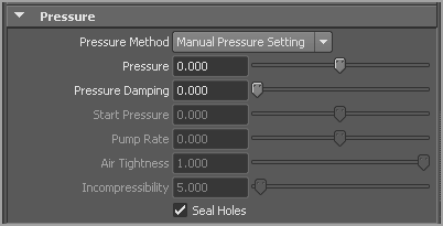
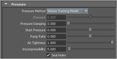
Manual Pressure Setting Manual Pressure Settingis simple—the Pressure slider and Pressure Damping slider are the only two controls (see
Figure 14-11). These can be keyframed to make it appear as though the nCloth object is being filled with air. If you set Pressure to 0 and create a keyframe, and then play the animation to frame 100, set Pressure to 1, and set another keyframe, the nCloth object will grow in size over those frames as if it were being inflated.
Volume Tracking Model Volume Tracking Model, which is used by the waterBalloon preset originally applied to the cell geometry, is a more accurate method for calculating volume and has more controls (see
Figure 14-12).
When Volume Tracking Model is selected as the pressure method, you have access to additional controls, such as Pump Rate, Air Tightness, and Incompressibility. The Pump Rate value determines the rate at which air is added within the volume. Positive values continue to pump air into the volume; negative values suck the air out. The Start Pressure value sets the initial pressure of the air inside the volume at the start of the animation.
The Air Tightness value determines the permeability of the nCloth object. Lower settings allow the air to escape the volume. The Incompressibility setting refers to the air within the volume. A lower value means the air is more compressible, which slows down the inflation effect of the cell. Activating Seal Holes causes the solver to ignore openings in the geometry.
As you may have noticed, after the cells divide in the example scene, they don’t quite return to the size of the original dividing cell. You can use the Pump Rate attribute to inflate the cells:
1. Continue with the scene from the previous section, or open the cellDivide_v04.ma scene from the chapter14scenes folder at the book’s web page.
2. Select the cellLeftCloth shape, and open its Attribute Editor.
3. Expand the Pressure settings. Note that Pressure Method is already set to Volume Tracking Model. These settings were determined by the waterBalloon preset originally used to create the effect.
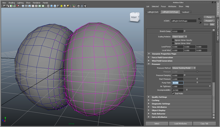
4. Set Pump Rate to
50 for each cell, and play the animation (see
Figure 14-13). Each cell starts to grow immediately and continues to grow after the cell divides.
5. Try setting keyframes on the start Pump Rate of both cells so that at frame 15 Pump Rate is 0, at frame 50 it’s 50, and at frame 100 it’s 0.
6. To give an additional kick at the start of the animation, set Start Pressure to 0.25.
Connect Attributes Using the Connection Editor
You can save some time by using the Connection Editor to connect the Pressure attributes of one of the cells to the same attributes of the other. This way, you only need to keyframe the attributes of the first cell. For more information on using the Connection Editor, consult Chapter 1, “Working in Autodesk Maya.”
Additional Techniques
To finish the animation, here are some additional techniques you can use to add some style to the behavior of the cells:
1. In the Collisions rollout, increase the Stickiness attribute of each cell to a value of 0.5. You can also try painting a Stickiness texture map. To do so, select the cells and choose nMesh ⇒ Paint Texture Properties ⇒ Stickiness. This activates the Artisan Brush, which allows you to paint specific areas of stickiness on the cell surface. (Refer to Chapter 13 to see how a similar technique is used to paint the strength of a force field on geometry.)
2. If you want the objects to start out solid and become soft at a certain point in time, set keyframes on each cell’s Input Mesh Attract attribute. The input mesh is the original geometry that was converted into the nCloth object. Setting the Input Mesh Attract attribute to 1 or higher causes the nCloth objects to assume the shape of the original geometry. As this value is lowered, the influence of the nucleus dynamics increases, causing the objects to become soft.
To see a finished version of the scene, open the cellDivide_v05.ma scene from the chapter14scenes folder at the book’s web page.
Combine Techniques
In practice, you’ll most likely find that the best solution when creating a complex effect is to combine techniques as much as possible. Use Dynamic Fields, Force, Wind, nConstraints, Air Density, Stickiness, and Pressure together to make a spectacular nCloth effect.
Creating an nCache
At this point, you’ll want to cache the dynamics so that playback speed is improved and the motion of the cells is the same every time you play the animation. Doing so also ensures that when you render the scene, the dynamics are consistent when using multiple processors.
Distributed Simulation
You can use the power of multiple computers to cache your simulations if you are using the Maya Entertainment Creation Suite. Backburner, which is part of the suite, must be installed and turned on. The distSim.py plug-in must also be loaded. You can then choose nCache ⇒ Send To Server Farm from the nDynamics menu set. Distributed simulation allows you to create variants of a single simulation and monitor its progress.
1. Shift+click the cellLeft and cellRight objects in the Outliner.
2. Choose nCache ⇒ Create New Cache ⇒ Options.
In the options, you can specify where the cache will be placed. By default, the cache is created in a subfolder of the current project’s Data folder. If the scene is going to be rendered on a network, make sure that the cache is in a subfolder that can be accessed by all the computers on the network.
In the options, you can specify whether you want to create a separate cache file for each frame or a single cache file. You can also create a separate cache for each geometry object; this is not always necessary when you have more than one nCloth object in a scene (see
Figure 14-14).
3. The default settings should work well for this scene. Click the Create button to create the cache. Maya will play through the scene.
After the nCache has been created, it is important that you disable the nCloth objects so that Maya does not calculate dynamics for objects that are cached. This is especially important for large scenes with complex nDynamics.
4. In the Attribute Editor for cellLeftClothShape, scroll to the top, and deselect the Enable button to disable the nCloth calculation. Do the same for cellRightClothShape.
Delete nCache Before Making Changes
When the cache is complete, the scene will play much faster. If you make changes to the nCloth settings, you won’t see the changes reflected in the animation until you delete or disable the nCache (nCache ⇒ Delete nCache). Even though the geometry is using a cache, you should not delete the nCloth nodes. This would disable the animation.
5. You can select the cellLeft and cellRight objects and move them so that they overlap at the center at the start of the scene. This removes the seam in the middle and makes it look as though there is a single object dividing into two copies.
6. You can also select the cellLeft and cellRight objects and smooth them using the Smooth operation in the Polygon ⇒ Mesh menu, or you can simply select the nCloth object and activate Smooth Mesh Preview by pressing the 3 key on the keyboard.
Cacheable Attributes
The specific attributes that are included in the nCache are set using the Cacheable Attributes menu in the Caching rollout found in the Attribute Editor for each nCloth object. You can use this menu to cache just the position or the position and velocity of each vertex from frame to frame. You also have the choice to cache the dynamic state of the nCloth object from frame to frame.
Caching the dynamic state means that the internal dynamic properties of the nCloth object are stored in the cache along with the position and velocity of each vertex. This means that if you decide to add more frames to the cache using the Append To Cache option in the nCache menu, you’re more likely to get an accurate simulation. This is because Maya will have more information about what’s going on inside the nCloth object (things such as pressure, collision settings, and so on) and will do a better job of picking up from where the original cache left off. This does mean that Maya will require more space on your hard drive to store this extra information.
Creating nCloth and nParticle Interactions
Creating dynamic interaction between nParticles and nCloth objects is quite easy because both systems can share the same Nucleus solver. Effects that were extremely difficult to create in previous versions of Maya are now simple to create, thanks to the collision properties of nDynamics. Before continuing with this section, review Chapter 13 so that you understand the basics of working with nParticles.
In this section, you’ll see how you can use nParticles to affect the behavior of nCloth objects. nCloth objects can be used to attract nParticles, nParticles can fill nCloth objects and cause them to tear open, and many interesting effects can be created by using nParticles and nCloth objects together.
Creating an nParticle Goal
Goal objects attract nParticles like a magnet. A goal can be a locator, a piece of geometry (including nCloth), or even another nParticle. In Chapter 13, you worked with force fields, which are similar to goals in some respects, in that they attract nParticles dynamically. Deciding whether you need to use a goal or a force field generated by an nDynamic object (or a combination of the two) depends on the effect you want to create and usually involves some experimentation. This section will demonstrate some uses of goal objects with some simple examples.
1. Create a new, empty scene in Maya.
2. Create a locator (Create ⇒ Locator).
3. Switch to the nDynamics menu set, and choose nParticles ⇒ Create nParticles ⇒ Balls to set the nParticle style to Balls.
4. Choose nParticles ⇒ Create nParticles ⇒ Create Emitter. By default, an omni emitter is created at the center of the scene.
5. Use the Move tool to position the emitter away from the locator (set Translate X, Y, and Z to 20).
6. Set the length of the timeline to 300.
7. Play the animation. Balls are emitted and fall through space because of the Gravity settings on the nucleus node.
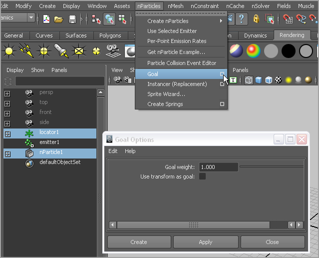
8. Select the nParticle object, and Ctrl/Command+click locator1. Choose nParticles ⇒ Goal ⇒ Options.
10. Rewind and play the scene.
The nParticles appear on the locator and bunch up over time. Since Goal Weight is set to 1, the goal is at maximum strength, and the nParticles move so quickly between the emitter and the goal object that they cannot be seen until they land on the goal. Since the Balls-style nParticles have Collision on by default, they stack up as they land on the goal.
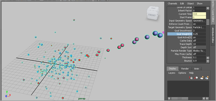
11. Select the nParticle object. In the Channel Box, set Goal Weight to
0.25. Play the animation. You can see the nParticles drawn toward the locator. They move past the goal and then move back toward it, where they bunch up and start to collide, creating a swarm (see
Figure 14-16).
12. Create a second locator. Position locator2 10 units above locator1.
13. Select the nParticle and Ctrl/Command+click locator2. Make it a goal with a weight of 0.25 as well.
14. Play the scene. The nParticles swarm between the two goals.
Multiple Goals
As goals are added to an nParticle, they are numbered according to the order in which they are added. The numbering starts at 0, so the first goal is referred to as Goal Weight[0], the second goal is referred to as Goal Weight[1], and so on. It’s a little confusing; sometimes it’s best to name the goal objects themselves using the same numbering convention. Name the first goal locator locatorGoal0, and name the second locatorGoal1. When adding expressions or when creating MEL scripts, this technique will help you keep everything clear.
15. Select one of the locators, and choose nSolver ⇒ Interactive Playback. You can move the locator in the scene while it’s playing and watch the nParticles follow. They are always drawn to the midpoint between the two goals (see
Figure 14-17).
16. Open the Attribute Editor for the nParticle, and switch to the nParticleShape1 tab. Try lowering the Conserve value on the nParticles. This causes the nParticles to lose energy as they fly through the scene.
17. Try these settings:
Conserve: 0.98
Drag: 0.05
Wind Speed on the Nucleus tab: 8
Wind Noise: 25
You can edit these settings in the Attribute Editor or in the Channel Box for the nParticleShape1 node. Suddenly a swarm of particles buzzes between the goal. By animating the position of the goals, you control where the swarm goes.
18. Enter the following settings:
Point Force Field on the nParticle node: World Space
Self Attract: -10
Point Field Distance: 10
Now the motion of the nParticles is controlled by the goals, gravity, wind, wind noise, and a force field generated by the nParticles themselves. You can quickly create complex behavior without the need for a single expression (see
Figure 14-18).
To see an example version of this scene, open the swarm.ma file from the chapter14scenes folder at the book’s web page. To see another example of the use of goals, open the nClothGoal.ma scene from the chapter14scenes folder.
Controlling Collision Events
Using the Collision Event Editor, you can specify what happens when a collision between an nParticle and a goal object occurs.
1. Open the nClothGoal.ma scene from the chapter14scenes folder.
2. Select the nParticle, and choose nParticles ⇒ Particle Collision Event Editor.
3. In the Editor window, select the nParticle. Leave the All Collisions check box enabled.
4. Set Event Type to Emit.
Split vs. Emit
The difference between Emit and Split is fairly subtle, but when Emit is selected, new particles are emitted from the point of collision, and you can specify that the original colliding nParticle dies. When you choose Split, the option for killing the original nParticle is unavailable.
5. Enter the following settings:
Num Particles: 5
Spread: 0.5
Inherit Velocity: 0.5
Check the Original Particle Dies option. Click Create Event to make the event (see
Figure 14-19).
Note that the collision event will create a new nParticle object.
6. Rewind and play the scene.
It may be difficult to distinguish the new nParticles that are created by the collision event from the original colliding nParticles. To fix this, continue with these steps:
7. Select nParticle2 in the Outliner, and open its Attribute Editor.
8. In the Particle Size rollout, set Radius to 0.05.
9. In the Shading rollout, set Color Ramp to a solid yellow.
10. Rewind and play the scene.
Each time an nParticle hits the nCloth object, it dies and emits three new nParticles. The nParticle2 node in the Outliner controls the behavior of and settings for the new nParticles. To see an example of this scene, open the collisionEvents.ma scene from the chapter14scenes folder at the book’s web page.
Bursting an Object Open Using Tearable nConstraints
This short example demonstrates how to create a bursting surface using nParticles and an nCloth surface.
1. In a new Maya scene, create a polygon cube at the center of the grid. The cube should have one subdivision in width, height, and depth.
2. Scale the cube up 8 units in each axis.
3. Select the cube, switch to the Polygon menu set, and choose Mesh ⇒ Smooth.
4. In the Channel Box, select the polySmoothFace1 node, and set Divisions to 3.
5. Select the cube, and switch to the nDynamics menu set.
6. Choose nMesh ⇒ Create nCloth to make the object an nCloth.
7. Open the Attribute Editor for the nCloth object, and use the Presets menu to apply the rubberSheet preset to the nCloth object.
8. Switch to the nucleus1 tab, and set Gravity to 0.
9. Choose nParticles ⇒ Create nParticles ⇒ Balls to set the nParticle style to Balls.
10. Choose nParticles ⇒ Create nParticles ⇒ Create Emitter to create a new emitter. By default, the emitter is placed at the origin inside the nCloth object.
11. Select the nParticles; in the Attribute Editor for the nParticleShape1 tab, expand the Particle Size rollout and set Radius to 0.5.
12. Set the length of the timeline to 800.
13. Rewind and play the animation. The nParticles start to fill up the surface, causing it to expand (see
Figure 14-20). If some nParticles are passing through the surface, switch to the Nucleus solver, and raise the Substeps value to
8.
14. Create a new shader, and apply it to the nCloth object.
15. Set the transparency of the shader to a light gray so that you can see the nParticles inside the nCloth object.
16. Select the pCube1 object in the Outliner.
17. Choose nConstraint ⇒ Tearable Surface. This applies a new nConstraint to the surface.
18. If you play the scene, you’ll see the surface burst open (see
Figure 14-21). Open the Attribute Editor for the nDynamic constraint. Set Glue Strength to
0.3 and Glue Strength Scale to
0.8; this will make the nConstraint more difficult to tear, so the bursting will not occur until around frame 500.
To see two examples of Tearable Surface nConstraints, open burst.ma and burst2.ma from the chapter14scenes folder at the book’s web page.
Designing Tearing Surfaces
You can specify exactly where you’d like the tearing to occur on a surface by selecting specific vertices before applying the Tearable Surface nConstraint.
Rigid Body Dynamics
Rigid body dynamics are the interactions of hard surfaces, such as the balls on a pool table, collapsing buildings, and links in a chain. The rigid body dynamic system in Maya has been part of the software since long before the introduction of nDynamics. In this section, you’ll learn how to set up a rigid body simulation and see how it can be used with nParticles to create the effect of a small tower exploding.
Creating an Exploding Tower
The example scene has a small tower of bricks on a hill. You’ll use a rigid body simulation to make the bricks of the tower explode outward on one side. Later, you’ll add nParticles to the simulation to create an explosion.
The scene is designed so that only one side of the tower will explode. Only a few stone bricks will be pushed out from the explosion; these bricks have been placed in the active group. The bricks in the passive group will be converted to passive colliders; they won’t move, but they will support the active brick. The bricks in the static group will be left alone. Since they won’t participate in the explosion, they won’t be active or passive, just plain geometry. This will increase the efficiency and the performance of the scene.
1. Open the tower_v01.ma scene in the chapter14scenes folder, expand the active group that’s inside the tower node, and select all the brick nodes in this group.
2. Switch to the Dynamics menu set (not the nDynamics menu set), and choose Soft/Rigid Bodies ⇒ Create Active Rigid Body.
3. Expand the passive group, Shift+click all the bricks in this group, and choose Soft/Rigid Bodies ⇒ Create Passive Rigid Body.
4. Select the ground, and choose Soft/Rigid Bodies ⇒ Create Passive Rigid Body.
By default, there is no gravity attached to the active rigid bodies; to add gravity, you need to create a gravity field.

5. Shift+click all the members of the active group, and choose Fields ⇒ Gravity.
If you play the scene, you’ll see the active bricks sag slightly. You actually don’t want them to move until the explosion occurs. To fix this, you can keyframe their dynamic state.
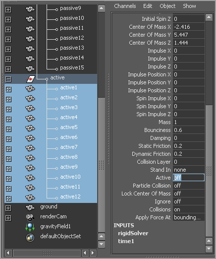
6. To animate their dynamic state, rewind the scene, Shift+click the members of the active group, and set the Active attribute in the Channel Box to Off (see
Figure 14-22).
7. Move the Time Slider to frame 19, right-click the Active channel, and choose Key Selected from the pop-up.
8. Move the timeline to frame 20, set Active to On, and set another keyframe.
9. To make the bricks explode, select the members of the active group, and add a radial field.
10. Position the radial field behind the active bricks, and enter the following settings:
Magnitude: 400
Attenuation: 0.5
Max Distance: 5
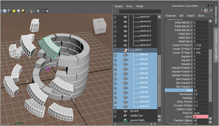
11. Select the active bricks, and set their Mass value to
20 (see
Figure 14-23).
When you play the scene, the bricks fly out at frame 20.
Interpenetration Errors
Interpenetration errors occur when two pieces of geometry pass through each other in such a way as to confuse Maya. Only one side of the surface is actually used in the calculation based on the direction of the surface normals—there are no double-sided rigid bodies. The surface of two colliding rigid bodies (active + active or active + passive) need to have their normals pointing at each other to calculate correctly.
To fix these errors, you can increase the Tessellation Factor value in the Performance Attributes rollout of each of the rigid body objects.
Also, you will notice that the bricks in the tower aren’t touching. When you model objects for a rigid body simulation, you’ll want to make sure that they all have some “breathing room” at the start so that the slightest movement won’t accidentally cause interpenetration.
Tuning the Rigid Body Simulation
You can tune the simulation by editing the settings on the active rigid bodies. The easiest way to do this for multiple objects is to select them all in the Outliner and then edit the settings in the Channel Box. For this example, you can decrease the amount of bouncing and sliding in the motion of the bricks by adjusting the bounciness and friction settings. There are two kinds of friction:
Static Friction Static Friction sets the level of resistance for a resting dynamic object against another dynamic object. In other words, if an object is stationary, this setting determines how much it resists starting to move once a force is applied.
Dynamic Friction Dynamic Friction sets how much a moving dynamic object resists another dynamic object, such as a book sliding across a table.
Other settings to note include Damping and Collision Layer. Damping slows down the movement of the dynamic objects. If the simulation takes place under water, you can raise this setting to make it look as though the objects are being slowed down by the density of the environment.
The Collision Layer specifies which objects collide with other objects. By default, all rigid bodies are on collision layer 0. However, if you set just the active bricks to collision layer 1, they react only with each other and not the ground or the passive bricks, which would still be on collision layer 0.
1. Select the ground plane, and set both the Static and Dynamic Friction attributes in the Channel Box to 1.
2. Shift+click the active bricks and, in the Channel Box, set Dynamic Friction to 0.5. Lower Bounciness to 0.1.
Rigid Body Solving Methods
Rigid bodies use the Rigid Solver node to calculate the dynamics. This node appears as a tab in the Attribute Editor when you select one of the rigid body objects, such as the bricks in the active group. The rigid solver uses one of three methods to calculate the dynamics: Mid-Point, Runge Kutta, and Runge Kutta Adaptive. Mid-Point is the fastest but least accurate, Runge Kutta is more accurate and slower, and Runge Kutta Adaptive is the most accurate and slowest method. In most cases, you can leave the setting on Runge Kutta Adaptive.
3. Save the scene as rigidBodyTower_v01.ma.
To see a version of the scene up to this point, open rigidBodyTower_v01.ma from the chapter14scenes folder.
Common Rigid Body Pitfalls
Moving objects with dynamics is very different than working with keyframed movement. For instance, you’ll notice that you can’t scrub through the timeline and see the motion properly update. This is because for the solver to function properly, it needs to calculate every frame and it can’t be rushed through the process. Because of this, you’ll want to make sure that you always have the playback speed of your scene set to Play Every Frame (right-click the timeline, and select Playback Speed ⇒ Play Every Frame, Max Real-Time).
In addition, you need to be careful when you group active rigid bodies. It makes sense at times to organize rigid bodies into groups, such as grouping the active body bricks in the tower. However, be careful not to transform these groups since the solver will become confused when it tries to move dynamic objects that have been scaled or moved around by a parent group.
Baking the Simulation
It’s common practice to bake the motion of traditional rigid bodies into keyframes once you’re satisfied that the simulation is working the way you want. This improves the performance of the scene and allows you to adjust parts of the animation by tweaking the keyframes on the Graph Editor.
1. In the Outliner, Shift+click the active bricks and choose Edit ⇒ Keys ⇒ Bake Simulation ⇒ Options.
2. In the Channel Box, Shift+click the Translate and Rotate channels.
3. In the Bake Simulation Options section, set Time Range to Time Slider.
4. Set the Channels option to From Channel Box. Keyframes are created for just the channels currently selected in the Channel Box. This eliminates the creation of extra, unnecessary keys.
5. Turn on Smart Bake. This setting tells Maya to create keyframes only where the animation requires it instead of creating a keyframe on every frame of the animation.
The Increase Fidelity option improves the accuracy of the smart bake. Fidelity Keys Tolerance specifies the baking tolerance in terms of a percentage. Higher percentages produce fewer keyframes but also allow for more deviation from the original simulation.
Other important options include the following:
Keep Unbaked Keys Keeps any key outside the baked range.
Sparse Curve Bake Keeps the shape of connected animation curves when baking. Since the bricks are using dynamics, this option does not apply.
Disable Implicit Control This option is useful when the object’s animation is being driven by Inverse Kinematic handles and other controls. This is not applicable when baking rigid body dynamics.
6. Activate Increase Fidelity, and set Fidelity Keys Tolerance to
1 percent (see
Figure 14-24).
7. Click the Bake button to bake the simulation into keyframes. The animation will play through as the keys are baked.
8. When the animation is finished, select Edit ⇒ Delete All By Type ⇒ Rigid Bodies to remove the rigid body nodes.
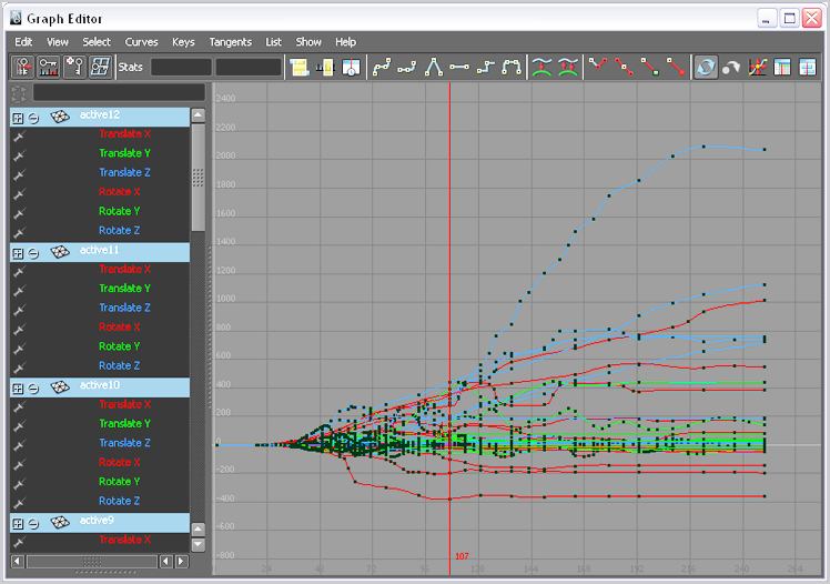
9. Select the active bricks, and open the Graph Editor (Window ⇒ Animation Editors ⇒ Graph Editor) to see the baked animation curves for the bricks (see
Figure 14-25).
10. If any of the bricks continue to wobble after landing on the ground, you can edit their motion on the Graph Editor by deleting the “wobbly” keyframes.
11. Save the scene as rigidBodyTower_v02.ma.
To see an example of the scene that uses traditional rigid bodies, open the rigidBodyTower_v02.ma scene from the chapter14scenes folder at the book’s web page.
Duplicating Traditional Rigid Bodies
When duplicating rigid bodies that have fields connected, do not use Duplicate Special ⇒ Duplicate Input Connections or Duplicate Input Graph. These options do not work well with rigid bodies. Instead, duplicate the object, convert it to an active rigid body, and then use the Relationship Editor to make the connection between the rigid bodies and the fields.
Crumbling Tower
nCloth objects can also be made into rigid objects. The advantage of doing this is that it allows you to make the nCloth objects semi-rigid. In addition, the setup can be easier. In Maya 2013, the ability to simulate polygon shells was added—combined geometry made into a single node—as if they were separate objects. The next project takes you through the steps.
1. Open the tower_v01.ma scene in the chapter14scenes folder.
2. Select a few well-chosen bricks from the tower and delete them (see
Figure 14-26).
3. Select the tower node, and choose Mesh ⇒ Combine from the Polygons menu set.
4. Delete the history, and rename the combined node back to tower.
5. Switch to the nDynamics menu set, and choose nMesh ⇒ Create nCloth.
6. Open nCloth1’s Attribute Editor.
7. Under Dynamic Properties, set Rigidity to
10.0 and check Use Polygon Shells (see
Figure 14-27).
8. Under the Collisions section, change Self Collision Flag to VertexEdge.
9. Select ground.
10. Choose nMesh Create Passive Collider.
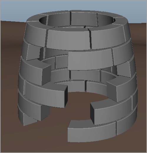
11. Play the simulation, and watch the tower crumble (see
Figure 14-28).
Try modifying the attributes to get the individual bricks to lose their shape as well. Hint: Use a low Deform Resistance value instead of Rigidity, and set Restitution Angle to 0.0.
Soft Body Dynamics
Soft body dynamics assign particles to each vertex of a polygon or NURBS object. The particles can be influenced by normal dynamic fields, such as air and gravity as well as rigid bodies. When influenced, the particles cause the vertices to follow, deforming the geometry.
There are two options for creating a soft body object. The first method is to make the geometry soft, which simply adds particles to every vertex. This allows the geometry to deform freely, never returning to its original shape. The second option is to make a duplicate, with one of the objects becoming a goal for the other. This method allows the geometry to return to its original shape. Using a goal is useful for creating objects that jiggle, like fat or Jell-O.
Use the following steps to create and adjust a soft body object:
1. Select a polygon or NURBS object.
2. Choose Soft/Rigid Bodies ⇒ Create Soft Body.
3. Set the Creation options to Duplicate, Make Copy Soft, and check Make Non-Soft A Goal. Choose Create.
With the soft body selected, you can add any field to influence the particles. Moving the original object will cause the soft body to follow. You can adjust the Goal Smoothness and Goal Weight on the particle node to alter the soft body’s behavior.
Bullet Physics
The MayaBullet physics plug-in is available only for 64-bit versions. Utilizing MayaBullet, you can create real-time game physics inside the Maya interface. Rigid bodies, rigid body constraints, and soft bodies are supported. In addition, you can create rigid body kinematics or ragdoll effects. These steps take you through the process:
1. Load the Bullet plug-in. Choose Window ⇒ Settings/Preferences ⇒ Plug-in Manager. Find bullet.mll (bullet.bundle on the Mac), and check Loaded and Auto Load.
2. Create a skeleton of a human character.
3. Make sure each joint is uniquely named. MayaBullet uses the names of your joints to create rigid capsules. If any of the names are duplicates, the capsules cannot be generated.
4. Select the root joint of your skeleton. Choose Bullet ⇒ Create Ragdoll From Skeleton.
5. Create a primitive plane at the skeleton’s feet. Choose Bullet ⇒ Create Passive Rigid Body.
6. Click the play button on the timeline to watch the simulation.
Creating Flying Debris Using nParticle Instancing
nParticle instancing attaches one or more specified pieces of geometry to a particle system. The instanced geometry then inherits the motion and much of the behavior of the particle system. For this example, you’ll instance debris and shrapnel to a particle system and add it to the current explosion animation. In addition, you’ll control how the instance geometry behaves through expressions and fields.
The goal for the exercises in this section is to add bits of flying debris to the explosion that behave realistically. This means that you’ll want debris of various sizes flying at different speeds and rotating as the particles move through the air. The first step is to add an nParticle system to the scene that behaves like debris flying through the air.
Adding nParticles to the Scene
The first step in creating the explosion effect is to add nParticles to the scene and make sure that they are interacting with the ground and the bricks of the tower. It’s a good idea to be efficient in your approach to doing this so that Maya is not bogged down in unnecessary calculations. To begin, you’ll add a volume emitter at the center of the tower.
1. Open the rigidBodyTower_v02.ma scene from the chapter14scenes folder. In this scene, the rigid body simulation has been baked into keyframes.
2. Switch to the nDynamics menu set, and choose nParticles ⇒ Create nParticles ⇒ Balls, to set the nParticle style to Balls.
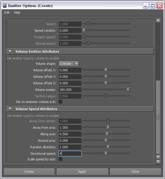
3. Choose nParticles ⇒ Create nParticles ⇒ Create Emitter ⇒ Options.
4. In the options, set Emitter Type to Volume, and Rate to 800.
5. In the Distance/Direction Attributes rollout, set Direction X and Direction Z to 0 and Direction Y to 1 so that the nParticles initially move upward.
6. In the Volume Emitter Attributes rollout, set Volume Shape to Cylinder.
7. In the Volume Speed Attributes rollout, enter the following settings:
Away From Axis: 1
Along Axis: 0.5
Random Direction: 1
Directional Speed: 4
9. Switch to wireframe mode. Select emitter1 in the Outliner, and use the Move and Scale tools to position the emitter at the center of the stone tower.
10. Set Translate Y to 3.1 and all three Scale channels to 2.
11. Rewind and play the animation.
The nParticles start pouring out of the emitter. They pass through the bricks and the ground.
12. Select the ground, and choose nMesh ⇒ Create Passive Collider.
13. Shift+click the bricks in the passive group, and convert them to passive colliders; do the same for the bricks in the active group.
The nParticles still pass through the static bricks at the back of the tower. You can convert the static bricks to passive colliders; however, this adds a large number of new nRigid nodes to the scene, which may slow down the performance of the scene. You can conserve some of the energy Maya spends on collision detection by creating a single, simple collider object to interact with the nParticles that hit the back of the tower. This object can be hidden in the render.
14. Switch to the Polygon menu set, and choose Create ⇒ Polygon Primitives ⇒ Cylinder.
15. Select the nParticle1 node and, in the Attribute Editor for the shape nodes, set Enable to Off to disable the calculations of the nParticle temporarily while you create the collision object.
16. Set the timeline to frame 100 so that you can easily see the opening in the exploded tower.
17. Set the scale and position of the cylinder so that it blocks the nParticles from passing through the back of the tower. Set the following:
Translate Y: 2.639
Scale X and Scale Z: 2.34
Scale Y: 3.5
18. Select the cylinder, and switch to face selection mode; delete the faces on the top and bottom of the cylinder and in the opening of the exploded tower (see
Figure 14-30).
19. Rename the cylinder collider. Switch to the nDynamics menu set, and choose nMesh ⇒ Create Passive Collider.
20. Select the nParticles, and turn Enable back on.
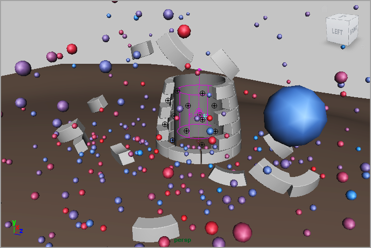
21. Rewind and play the animation; the nParticles now spill out of the front of the tower once it breaks open (see
Figure 14-31).
22. Save the scene as explodingTower_v01.ma.
To see a version of the scene up to this point, open the explodingTower_v01.ma scene from the chapter14scenes folder at the book’s web page.
Sending the Debris Flying Using a Field
So far, the effects look like a popcorn popper gone bad. To make it look as though the nParticles are expelled from the source of the explosion, you can connect the radial field to the nParticle.
1. Continue with the scene from the previous section, or open explodingTower_v01.ma from the chapter14scenes folder at the book’s web page. Select nParticle1, and rename it particleDebris.
2. Open the Attribute Editor for particleDebris. Switch to the nucleus1 tab.
3. In the Time Attributes rollout, set Start Frame to 20 so that the emission of the nParticles is in sync with the exploding brick.
It’s not necessary to have the debris continually spewing from the tower. You need only a certain number of nParticles. You can either set keyframes on the emitter’s rate or set a limit to the number of nParticles created by the emitter. The latter method is easier to do and to edit later.
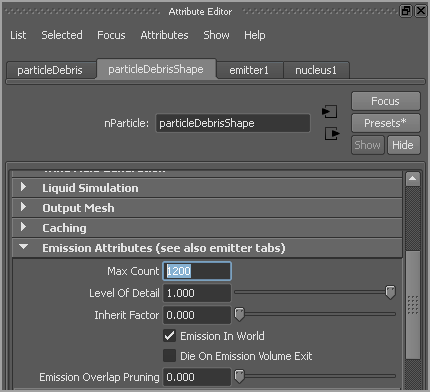
4. In the Attribute Editor for particleDebrisShape, expand the Emission Attributes rollout. Max Count is set to –1 by default, meaning that the emitter can produce an infinite number of nParticles. Set this value to
1200(see
Figure 14-32).
5. After the number of nParticles reaches 1200, the emitter stops creating new nParticles. Select the emitter, and set the rate to 2400. This means that the emitter will create 1,200 nParticles in half a second, making the explosion faster and more realistic.
Max Count and nParticle Death
This method works well as long as the nParticles do not have a finite life span. If there is a life span set for the nParticles or if they die from a collision event, the emitter creates new nParticles to make up the difference.
6. You can connect the particleDebris node to the existing radial field that was used to push out the bricks. To connect the radial field to the particleDebris node, select the particleDebris node and Ctrl/Command+click radialField1 in the Outliner. Choose Fields ⇒ Affect Selected Object(s).
Making Connections with the Relationship Editor
You can also connect the field to the nParticle using the Dynamic Relationship Editor. This is discussed in Chapter 13.
7. Rewind and play the animation. Not all the nParticles make it out of the tower; many of the nParticles are pushed down on the ground and toward the back of the collider object. To fix this, reposition the radial field.
8. Set the Translate X of the field to
1.347 and the Translate Y to
0.364 (see
Figure 14-33).
9. Save the scene as explodingTower_v02.ma.
To see a version of the scene up to this point, open the explodingTower_v02.ma scene from the chapter14scenes folder at the book’s web page.
Creating a More Convincing Explosion by Adjusting nParticle Mass
Next, to create a more convincing behavior for the nParticles, you can randomize the mass. This means that there will be random variation in how the nParticles move through the air as they are launched by the radial field.
1. Select the particleDebris node in the Outliner, and open its shape node in the Attribute Editor.
2. Under the Dynamic Properties rollout, you can leave Mass at a value of 1. In the Mass Scale settings, set Mass Scale Input to Randomize ID. This randomizes the mass of each nParticle using its ID number as a seed value to generate the random value.
3. If you play the animation, the mass does not seem all that random. To create a range of values, add a point to the Mass Scale ramp on the right side, and bring it down to a value of 0.1.
When Mass Scale Input is set to Randomize ID, you can alter the range of variation by adjusting the Input Max slider. If you think of the Mass Scale ramp as representing possible random ranges, lowering Input Max shrinks the available number of random values to the randomize function, thus forcing the randomizer to have more “contrast” between values. Increasing Input Max makes more data points available to the randomize function, making a smoother variation between random values and producing less contrast (see
Figure 14-34).
4. Set the Input Max slider to 0.5.
The Input Max slider is part of the Mass Scale Input options. The slider is an additional randomization value that is multiplied against the initial mass value, such as that if you set Mass Scale Input to speed or age or acceleration, or you can use the slider to add some random variation to the mass. You don’t need to use this slider if the Mass Scale input is set to Randomize ID, and sometimes it can result in creating random values so close to 0 that the nParticles end up getting stuck in the air.
5. Create a playblast of the scene so that you can see how the simulation is working so far.
The nParticles are sliding along the ground in a strange way. To make them stop, you can increase the stickiness and friction of the ground.
6. Select the ground geometry, and open its Attribute Editor.
7. Switch to the nRigidShape1 tab. Under the Collisions rollout, set Stickiness to 1 and Friction to 0.2.
8. Save the scene as explodingTower_v03.ma.
To see a version of the scene, open explodingTower_v03.ma from the chapter14scenes folder at the book’s web page.
Instancing Geometry
The debris is currently in the shape of round balls, which is not very realistic. To create the effect of flying shrapnel, you’ll need to instance some premade geometry to each nParticle. This means that a copy of each piece of geometry will follow the motion of each nParticle.
1. Continue using the scene from the previous section, or open the explodingTower_v03.ma scene from the chapter14scenes folder.
2. The debris is contained in a separate file, which will be imported into the scene. Choose File ⇒ Import, and select the debris.ma scene from the chapter14scenes folder at the book’s web page.
The debris scene is simply a group of seven polygon objects in the shape of shards.
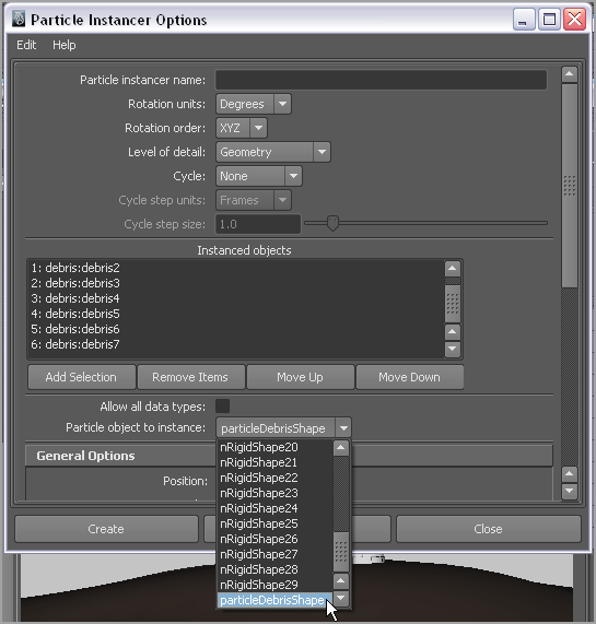
3. Expand the debris:debris group in the Outliner, Shift+click all the members of the group, and choose nParticles ⇒ Instancer (Replacement) ⇒ Options.
In the Options window, all the debris objects are listed in the order in which they were selected in the Outliner. Notice that each one has a number to the left in the list. This number is the index value of the instance. The numbering starts with 0.
4. In the Particle Object To Instance drop-down menu, choose the particleDebrisShape object. This sets the instance to the correct nDynamic object (see
Figure 14-35).
5. Leave the rest of the settings at their defaults, and choose Create to instance the nParticles. In the Outliner, a new node named instance1 has been created.
6. Play the scene. Switch to wireframe mode, and zoom in closely to the nParticles so that you can see what’s going on.
7. Save the scene as explodingTower_v04.ma.
To see a version of the scene up to this point, open the explodingTower_v04.ma scene from the chapter14scenes folder at the book’s web page.
When playing the scene, you’ll notice that each nParticle has the same piece of geometry instanced to it, and they are all oriented the same way (see Figure 14-36). To randomize which objects are instanced to the nParticles and their size and orientation, you’ll need to create some expressions. In the next section, you’ll learn how to assign the different objects in the imported debris group randomly to each nParticle as well as how to make them rotate as they fly through the air. You will also learn how to use each nParticle’s mass to determine the size of the instanced geometry. All of this leads to a much more realistic-looking explosion.
Tips for Working with nParticle Instances
Geometry that is instanced to nParticles inherits the position and orientation of the original geometry. If you place keyframes on the original geometry, this is inherited by the instanced copies.
If you’re animating flying debris, it’s a better idea to animate the motion of the instances using expressions and the dynamics of the nParticles rather than setting keyframes of the rotation or translation of the original instanced geometry. This approach makes animation simpler and allows for more control when editing the effect.
It’s also best to place the geometry you want to instance at the origin and place its pivot at the center of the geometry. You’ll also want to freeze transformations on the geometry to initialize its translation, rotation, and scale attributes.
In some special cases, you may want to offset the pivot of the instanced geometry. To do this, position the geometry away from the origin of the grid, place the pivot at the origin, and freeze transformations.
If you are animating crawling bugs or the flapping wings of an insect, you can animate the original geometry you want to instance, or you can create a sequence of objects and use the Cycle feature in the instance options. The Cycle feature causes the instance to progress through a sequence of geometry based on the index number assigned to the instanced geometry. The Cycle feature offers more flexibility than simply animating the instanced geometry. You can use expressions to randomize the start point of the cycle on a per-particle basis. nParticle expressions are covered in the next section.
You can add more objects to the Instanced Objects list after creating the instance using the options in the Attribute Editor for the instance node.
Animating Instances Using nParticle Expressions
nParticles allow you to create more interesting particle effects than in previous versions of Maya without relying on expressions. However, in some situations, expressions are still required to achieve a believable effect. If you’ve never used particle expressions, they can be a little intimidating at first, and the workflow is not entirely intuitive. Once you understand how to create expressions, you can unleash an amazing level of creative potential; combine them with the power of the Nucleus solver, and there’s almost no effect you can’t create. Expressions work the same way for both nParticles and traditional Maya particles.
Randomizing Instance Index
The first expression you’ll create will randomize which instance is copied to which nParticle. To do this, you’ll need to create a custom attribute. This custom attribute will assign a random value between 0 and 6 for each nParticle, and this value will be used to determine the index number of the instance copied to that particular particle.
1. Select the particleDebris node in the Outliner, and open its Attribute Editor to the particleDebrisShape tab.
2. Scroll down and expand the Add Dynamic Attributes rollout.
3. Click the General button; a pop-up dialog box appears (see
Figure 14-37). This dialog box offers you options to determine what type of attribute will be added to the particle shape.
4. In the Long Name field, type debrisIndex. This is the name of the attribute that will be added to the nParticle.
Naming an Attribute
You can name an attribute anything you want (as long as the name does not conflict with a preexisting attribute name). It’s best to use concise names that make it obvious what the attribute does.
5. Set Data Type to Float. A float is a single numeric value that can have a decimal. Numbers like 3, 18.7, and –0.314 are examples of floats.
6. Set Attribute Type to Per Particle (Array).
Per Particle vs. Scalar Attributes
A per-particle attribute contains a different value for each particle in the particle object. This is opposed to a scalar attribute, which applies the same value for all the particles in the particle object. For example, if an nParticle object represented an American president, a per-particle attribute would be something like the age of each president when elected. A scalar attribute would be something like the nationality of the presidents, which would be American for all of them.
7. Click OK to add the attribute.
Now that you have an attribute, you need to create the expression to determine its value:
1. Expand the Per Particle (Array) Attributes rollout, and you’ll see Debris Index listed.
2. Right-click the field next to Debris Index, and choose Creation Expression (see
Figure 14-38).
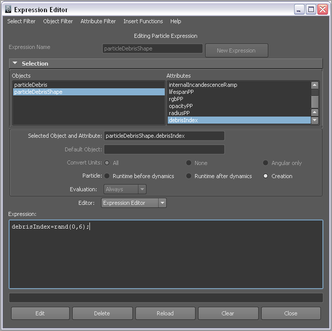
The Expression Editor opens, and debrisIndex is selected in the Attributes list. Notice that the Particle mode is automatically set to Creation.
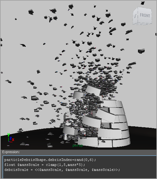
3. In the Expression field, type
debrisIndex=rand(0,6); (see
Figure 14-39). Remember that the list of instanced objects contains seven objects, but the index list starts with 0 and goes to 6.
This adds a random function that assigns a number between 0 and 6 to the debrisIndex attribute of each nParticle. The semicolon at the end of the expression is typical scripting syntax and acts like a period at the end of a sentence.
4. Click the Create button to create the expression.
5. Rewind and play the animation.
Nothing has changed at this point—the same piece of debris is assigned to all the nParticles. This is because, even though you have a custom attribute with a random value, you haven’t told Maya how to apply the attribute to the particle.
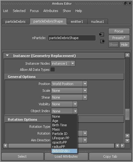
6. Expand the Instancer (Geometry Replacement) rollout in the Attribute Editor of particleDebrisShape.
7. In the General Options section, expand the Object Index menu and choose debrisIndex from the list (see
Figure 14-40).
Now when you rewind and play the animation, you’ll see a different piece of geometry assigned to each nParticle.
8. Save the scene as explodingTower_v05.ma.
To see a version of the scene up to this point, open the explodingTower_v05.ma scene from the chapter14scenes folder at the book’s web page.
Creation vs. Runtime Expressions
There are two types of expressions you can create for a particle object: creation and runtime. The difference between creation and runtime is that creation expressions evaluate once when the particles are created (or at the start of the animation for particles that are not spawned from an emitter), and runtime expressions evaluate on each frame of the animation for as long as they are in the scene.
A good way to think of this is that a creation expression is like a trait determined by your DNA. When you’re born, your DNA may state something like “Your maximum height will be 6 feet, 4 inches.” So, your creation expression for height would be “maximum height = 6 feet, 4 inches.” This has been set at the moment you are created and will remain so throughout your life unless something changes.
Think of a runtime expression as an event in your life. It’s calculated each moment of your life. If for some reason during the course of your life your legs were replaced with bionic extend-o-legs that give you the ability to change your height automatically whenever you want, this would be enabled using a runtime expression. It happens after you have been born and can override the creation expression. Thus, at any given moment (or frame in the case of particles), your height could be 5 feet or 25 feet, thanks to your bionic extend-o-legs.
If you write a creation expression for the particles that says radius = 2, each particle will have a radius of 2, unless something changes. If you then add a runtime expression that says something like “If the Y position of a particle is greater than 10, then radius = 4,” any particle that goes beyond 10 units in Y will instantly grow to 4 units. The runtime expression overrides the creation expression and is calculated at least once per frame as long as the animation is playing.
Connecting Instance Size to nParticle Mass
Next you’ll create an expression that determines the size of each nParticle based on its mass. Small pieces of debris that have a low mass will float down through the air. Larger pieces that have a higher mass will be shot through the air with greater force. The size of instances is determined by their Scale X, Scale Y, and Scale Z attributes, much like a typical piece of geometry that you work with when modeling in Maya. This is different from a Balls-type nParticle that uses a single radius value to determine its size.
The size attributes for instanced geometry are contained in a vector. A vector is an attribute with a three-dimensional value, as opposed to an integer or a float, which has only a single-dimensional value.
1. Select the particleDebris object and, in the shape node’s Attribute Editor, under Add Dynamic Attributes click the General button to create a new attribute.
2. Set the Long Name value to debrisScale.
3. Set Data Type to Vector and Attribute Type to Per Particle (Array), and click OK to make the attribute (see
Figure 14-41).
4. In the Per Particle (Array) Attributes section, right-click the field next to debrisScale, and choose to create a creation expression.
Refresh the Attribute List
If the new attribute does not appear in the list, click the Load Attributes button at the bottom of the Attribute Editor to refresh the list.
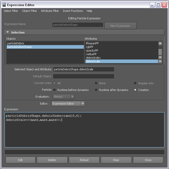
In the Expression field of the Expression Editor, you’ll see the debrisIndex expression. Note that the name debrisIndex has been expanded; it now says particleDebrisShape.debrisIndex=rand(0,6);. Maya does this automatically when you create the expression.
5. Below the debrisIndex expression, type
debrisScale=<<mass,mass,mass>>;. Click Edit to add this to the expression (see
Figure 14-42).
The double brackets are the syntax used when specifying vector values. Using mass as the input value for each dimension of the vector ensures that the pieces of debris are uniformly scaled.
6. In the Instancer (Geometry Replacement) attributes of the particleDebris object, set the Scale menu to debrisScale (see
Figure 14-43).
7. Rewind and play the animation.
The pieces of debris are now sized based on the mass of the nParticles, but of course the mass of some of the particles is so small that the instanced particles are invisible. To fix this, you can edit the expression, as follows:
1. In the Per-Particle (Array) Attributes section, right-click debrisScale, and choose Creation Expression to open the Expression Editor.
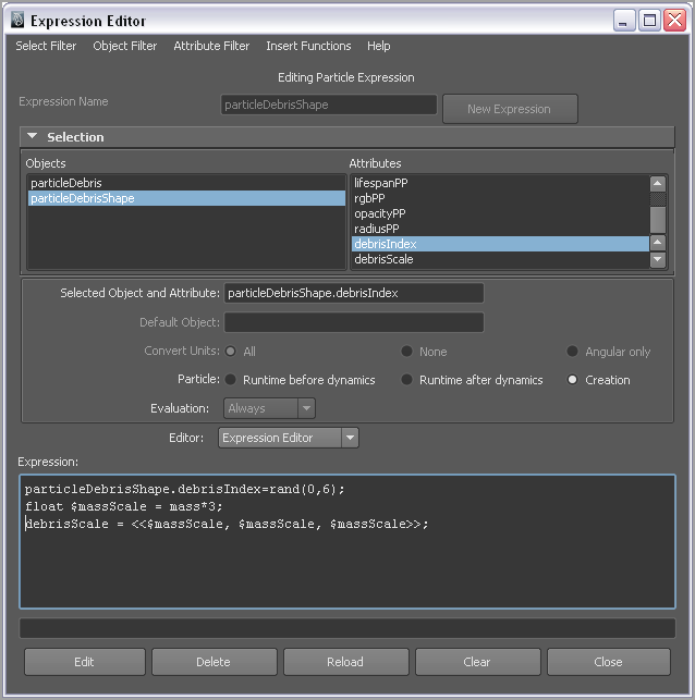
2. In the Expression field, add the following text above the debris scale expression:
float $massScale = mass*3;
3. Now edit the original debrisScale expression, as shown in
Figure 14-44, so it reads as follows:
debrisScale = <<$massScale, $massScale, $massScale>>;
By using the float command in the Expression Editor, you’re creating a local variable that is available to be used only in the creation expressions used by the nParticle. This variable is local, meaning that, since it was created in the Creation expression box, it’s available only for creation expressions. If you use this variable in a runtime expression, Maya gives you an error message. The variable is preceded by a dollar sign. The $massScale variable is assigned the mass multiplied by 3.
4. Click Edit to implement the changes to the expression.
5. Rewind and play the animation.
It’s an improvement; some debris pieces are definitely much bigger, but some are still too small. You can fix this by adding a clamp function. clamp sets an upper and lower limit to the values generated by the expression. The syntax is clamp(lower limit, upper limit, input);. Make sure you click the Edit button in the editor after typing the expression.
6. Edit the expression for the massScale variable so that it reads float $massScale=clamp(1,5,mass*5);. Make sure that you click the Edit button in the editor after typing the expression.
7. Play the animation.
Now you have a reasonable range of sizes for the debris, and they are all based on the mass on the particles (see
Figure 14-45).
8. In the Attribute Editor for the particleDebris, scroll to the Shading section and set Particle Render Type to Points so that you can see the instanced geometry more easily.
9. Save the scene as explodingTower_v06.ma.
To see a version of the scene, open the explodingTower_v06.ma scene from the chapter14scenes folder at the book’s web page.
Controlling the Rotation of nParticles
Rotation attributes are calculated per particle and can be used to control the rotation of geometry instanced to the nParticles. In addition, the Rotation Friction and Rotation Damp attributes can be used to fine-tune the quality of the rotation. In this exercise, you’ll add rotation to the debris:
1. Continue with the scene from the previous section, or open the explodingTower_v06.ma scene from the chapter14scenes folder at the book’s web page.
2. Select the particleDebris node in the Outliner, and open its Attribute Editor to the particleDebrisShape tab.
3. Expand the Rotation tab, and turn on Compute Rotation (see
Figure 14-46). This automatically adds a new attribute to the Per Particle Array Attributes list. However, you won’t need to create any expressions in order to make the nParticle rotate.
4. Scroll down to the Instancer (Geometry Replacement) settings. In the Rotation Options, set the Rotation menu to rotationPP.
5. Create a playblast of the scene.
6. You may notice that some of the debris rotates a bit too quickly as it falls to Earth. To adjust this, scroll up to the Rotation section, and set Rotation Damp to 0.01. Try making another playblast.
7. Save the scene as explodingTower_v07.ma.
Rotation Friction and Rotation Damp are per-particle attributes, which can be used in per-particle expressions to drive other attributes:
Rotation Friction This attribute determines how likely an nParticle will rotate based on its collision with other nDynamic objects and self-collisions (inter-particle collisions within the same nParticle shape). Setting Rotation Friction to 0 turns off rotation.
Rotation Damp This attribute causes the rotation of nParticles to slow down after collisions with other nDynamic objects and self-collisions.
To see a version of the scene, open the explodingTower_v07.ma scene from the chapter14scenes folder at the book’s web page.
Caching Instanced nParticles
When creating an nCache for nParticles that have geometry instanced to them or any nParticle with custom attributes and expressions, be sure to set the Cacheable Attributes menu in the Caching rollout of the nParticle’s Attribute Editor, to All. Otherwise, the cache will store only position and velocity data, and the motion of the nParticles will not look correct when you render the scene.
The Bottom Line
Use nCloth nCloth can be used to make polygon geometry behave dynamically to simulate a wide variety of materials. Using the presets that come with Maya, you can design your own materials and create your own presets for use in your animations.
Master It Create the effect of a cube of gelatinous material rolling down the stairs.
Combine nCloth and nParticles Because nCloth and nParticles use the same dynamic systems, they can be combined easily to create amazing simulations.
Master It Make a water balloon burst as it hits the ground.
Use Maya rigid body dynamics Rigid body dynamics are not quite as powerful as nCloth objects, but they do calculate much faster and work better for simulations involving a large number of interacting pieces.
Master It Animate a series of dominoes falling over.
Use nParticles to drive instanced geometry Modeled geometry can be instanced to nParticles to create a wide variety of effects.
Master It Create the effect of a swarm of insects attacking a beach ball.
Create nParticle expressions nParticle expressions can be used to further extend the power of nParticles. Using expressions to automate instanced geometry simulations is just one of the ways in which expressions can be used.
Master It Improve the animation of the insects attacking the beach ball by adding different types of insects to the swarm. Randomize their size, and create expressions so that larger insects move more slowly.