Chapter 3
Modeling I
Creating 3D models in computer graphics is an art form and a discipline unto itself. It takes years to master and requires an understanding of form, composition, anatomy, mechanics, and gesture. It’s an addictive art that never stops evolving. With a firm understanding of how the tools work, you can master the art of creating 3D models.
The Autodesk® Maya® software supports three types of surfaces: polygon, NURBS, and subdivisions. Each is quite different and has its strengths and weaknesses. Polygon models are constructed by attaching flat geometric shapes together to form a volume. There are few restrictions when working with polygons, and for this reason they are more popular than NURBS as a modeling tool. A NURBS surface is created by spreading a three-dimensional surface across a network of NURBS curves. NURBS and polygons are not mutually exclusive. As an artist, you can combine the two types of surfaces and take advantage of the strengths of both. Subdivision surfaces are like a hybrid of NURBS and polygon surfaces.
This chapter and the next demonstrate various techniques for modeling with polygons, NURBS surfaces, and subdivision surfaces to create a model of a space suit.
In this chapter, you will learn to:
- Understand polygon geometry
- Understand subdivision surfaces
- Understand NURBS surfaces
- Employ image planes
- Model with NURBS surfaces
- Use NURBS tessellation
- Model with polygons
Understanding Polygon Geometry
Polygon geometry refers to a surface made up of polygon faces that share edges and vertices. A polygon face is a geometric shape consisting of three or more edges. Vertices are points along the edges of polygon faces, usually at the intersection of two or more edges.
Many tools are available that allow you to make arbitrary changes (such as splitting, removing, and extruding) to polygon faces. Polygons are versatile. They can be used to create hard-surface models, such as vehicles, armor, and other mechanical objects, as well as organic surfaces, such as characters, creatures, and other natural objects. Before you get started working on the space suit, it’s a good idea to gain an understanding of the basic components of a polygon surface.
Polygon Vertices
A polygon is a surface constructed using three or more points known as vertices. The surface between these vertices is a face. A mesh is a series of faces that share two or more vertices. The most common way to create a polygon surface is to start with a primitive (such as a plane, sphere, or cube) and then use the numerous editing tools to shape the primitive gradually into the object that you want to create.
When all the vertices of a polygon are along a single plane, the surface is referred to as planar. When the vertices are moved to create a fold in the surface, the surface is referred to as nonplanar(see Figure 3-1). It’s usually best to keep your polygon surfaces as planar as possible. This strategy helps you avoid possible rendering problems, especially if the model is to be used in a video game. As you’ll see in this chapter, you can use a number of tools to cut and slice the polygon to reduce nonplanar surfaces.
Polygon Edges
The line between two polygon vertices is an edge. You can select one or more edges and use the Move, Rotate, and Scale tools to edit a polygon surface. Edges can also be flipped, deleted, or extruded. Having this much flexibility can lead to problematic geometry. For instance, you can extrude a single edge so that three polygons share the same edge (see Figure 3-2).
This configuration is known as a nonmanifold surface, and it’s a situation to avoid. Some polygon-editing tools in Maya do not work well with nonmanifold surfaces, and they can lead to rendering and animation problems. Another example of a nonmanifold surface is a situation where two polygons share a single vertex but not a complete edge, creating a bow-tie shape (see Figure 3-3).
Polygon Faces
The actual surface of a polygon is known as a face. Faces are what appear in the final render of a model or animation. There are numerous tools for editing and shaping faces, which are explored throughout this chapter and the next one.
Take a look at Figure 3-4. You’ll see a green line poking out of the center of each polygon face. This line indicates the direction of the face normal; essentially, it’s where the face is pointing.
The direction of the face normal affects how the surface is rendered; how effects such as dynamics, hair, and fur are calculated; and other polygon functions. Many times, if you are experiencing strange behavior when working with a polygon model, it’s because there is a problem with the normals (see Figure 3-5). You can usually fix this issue by softening or reversing the normals.
Two adjacent polygons with their normals pointing in opposite directions is a third type of nonmanifold surface. Try to avoid this configuration.
Working with Smooth Polygons
There are two ways to smooth a polygon surface: you can use the Smooth operation (from the Polygons menu set, choose Mesh ⇒ Smooth), or you can use the Smooth Mesh Preview command (select a polygon object, and press the 3 key).
When you select a polygon object and use the Smooth operation in the Mesh menu, the geometry is subdivided. Each level of subdivision quadruples the number of polygon faces in the geometry and rounds the edges of the geometry. This also increases the number of polygon vertices available for manipulation when shaping the geometry (see Figure 3-6).
When you use the smooth mesh preview, the polygon object appears smooth; however, it is not subdivided. Think of this as a mode where you can preview the polygon surface as if you had used the Smooth option in the Mesh menu (which is why it’s called smooth mesh preview).
When a polygon surface is in smooth mesh preview mode, the number of vertices available for manipulation remains the same as in the original unsmoothed geometry; this simplifies the modeling process.
- To create a smooth mesh preview, select the polygon geometry, and press the 3 key.
- To return to the original polygon mesh, press the 1 key.
- To see a wireframe of the original mesh overlaid on the smooth mesh preview (see Figure 3-7), press the 2 key.
The terms smooth mesh preview and smooth mesh polygons are interchangeable; both are used in this book and in the Maya interface.
When you render polygon geometry as a smooth mesh preview using mental ray, the geometry appears smoothed in the render without the need to convert the smooth mesh to standard polygons or change it in any way. This makes modeling and rendering smooth and organic geometry with polygons much easier.
Using Subdivision Surfaces
The Maya subdivision surfaces are very similar to the polygon smooth mesh preview. The primary distinction between smooth mesh preview and subdivision surfaces (subDs) is that subdivision surfaces allow you to subdivide a mesh to add detail only where you need it. For instance, if you want to sculpt a fingernail at the end of a finger, using subDs you can select just the tip of the finger and increase the subdivisions. Then you have more vertices to work just at the fingertip, and you can sculpt the fingernail.
Most subD models start out as polygons and are converted to subDs only toward the end of the modeling process. You should create UV texture coordinates while the model is still made of polygons. They are carried over to the subDs when the model is converted.
So why are subDs and smooth mesh preview polygons so similar, and which should you use? SubDs have been part of Maya for many versions. Smooth mesh preview polygons have only recently been added to Maya; thus, the polygon tools have evolved to become very similar to subDs. You can use either type of geometry for many of the same tasks; it’s up to you to decide when to use one rather than another.
When you convert a polygon mesh to a subdivision surface, you should keep in mind the following:
- Keep the polygon mesh as simple as possible; converting a dense polygon mesh to a subD significantly slows down performance.
- You can convert three-sided or n-sided (four- or more-sided) polygons into subDs, but you will get better results and fewer bumps in the subD model if you stick to four-sided polygons as much as possible.
- Nonmanifold geometry is not supported. You must alter this type of geometry before you are allowed to do conversion.
Understanding NURBS
NURBS is an acronym that stands for Non-Uniform Rational B-Spline. As a modeler, you need to understand a few concepts when working with NURBS, but the software takes care of most of the advanced mathematics so that you can concentrate on the process of modeling.
Early in the history of 3D computer graphics, NURBS were used to create organic surfaces and even characters. However, as computers have become more powerful and the software has developed more advanced tools, most character modeling is accomplished using polygons and subdivision surfaces. NURBS are more ideally suited for hard-surface modeling; objects such as vehicles, equipment, and commercial product designs benefit from the types of smooth surfacing produced by NURBS models.
All NURBS objects are automatically converted to triangles at render time by the software. You can determine how the surfaces will be tessellated (converted into triangles) before rendering, and you can change these settings at any time to optimize rendering. This gives NURBS the advantage that their resolution can be changed when rendering. Models that appear close to the camera can have higher tessellation settings than those farther away from the camera.
One of the downsides of NURBS is that the surfaces themselves are made of four-sided patches. You cannot create a three- or five-sided NURBS patch, which can sometimes limit the kinds of shapes you can make with NURBS. If you create a NURBS sphere and use the Move tool to pull apart the control vertices at the top of the sphere, you’ll see that even the patches of the sphere that appear as triangles are actually four-sided panels (see Figure 3-8).
Understanding Curves
All NURBS surfaces are created based on a network of NURBS curves. Even the basic primitives, such as the sphere, are made up of circular curves with a surface stretched across them. The curves themselves can be created several ways. A curve is a line defined by points. The points along the curve are referred to as curve points. Movement along the curve in either direction is defined by its U-coordinates. When you right-click a curve, you can choose to select a curve point. The curve point can be moved along the U-direction of the curve, and the position of the point is defined by its U-parameter.
Curves also have edit points that define the number of spans along a curve. A span is the section of the curve between two edit points. Changing the position of the edit points changes the shape of the curve; however, this can lead to unpredictable results. It is a much better idea to use a curve’s control vertices to edit the curve’s shape.
Control vertices (CVs) are handles used to edit the curve’s shapes. Most of the time you’ll want to use the control vertices to manipulate the curve. When you create a curve and display its CVs, you’ll see them represented as small dots. The first CV on a curve is indicated by a small box; the second is indicated by the letter U.
Hulls are straight lines that connect the CVs; they act as a visual guide.
Figure 3-9 displays the various components.
The degree of a curve is determined by the number of CVs per span minus one. In other words, a three-degree (or cubic) curve has four CVs per span. A one-degree (or linear) curve has two CVs per span (see Figure 3-10). Linear curves have sharp corners where the curve changes directions; curves with two or more degrees are smooth and rounded where the curve changes direction. Most of the time, you’ll use either linear (one-degree) or cubic (three-degree) curves.
You can add or remove a curve’s CVs and edit points, and you can also use curve points to define a location where a curve is split into two curves or joined to another curve.
The parameterization of a curve refers to the way in which the points along the curve are numbered. There are two types of parameterization:
Uniform Parameterization A curve with uniform parameterization has its points evenly spaced along the curve. The parameter of the last edit point along the curve is equal to the number of spans in the curve. You also have the option of specifying the parameterization range between 0 and 1. This method is available to make Maya more compatible with other NURBS modeling programs.
Chord Length Parameterization Chord length parameterization is a proportional numbering system that causes the length between edit points to be irregular. The type of parameterization you use depends on what you are trying to model. Curves can be rebuilt at any time to change their parameterization; however, this will sometimes change the shape of the curve.
You can rebuild a curve to change its parameterization (using the Surfaces menu set under Edit Curves ⇒ Rebuild Curve). It’s often a good idea to do this after splitting a curve or joining two curves together, or when matching the parameterization of one curve to another. By rebuilding the curve, you ensure that the resulting parameterization (Min and Max Value attributes in the curve’s Attribute Editor) is based on whole-number values, which leads to more predictable results when the curve is used as a basis for a surface. When rebuilding a curve, you have the option of changing the degree of the curve so that a linear curve can be converted to a cubic curve, and vice versa.
Bézier Curves
Bézier curves use handles for editing as opposed to CVs that are offset from the curve. To create a Bézier curve, choose Create ⇒ Bezier Curve. Each time you click the perspective view, a new point is added. To extend the handle, LMB-drag after adding a point. The handles allow you to control the smoothness of the curve. The advantage of Bézier curves is that they are easy to edit, and you can quickly create curves that have both sharp corners and rounded curves.
Importing Curves
You can create curves in Adobe Illustrator and import them into Maya for use as projections on the model. For best results, save the curves in Illustrator 8 format. In Maya, choose File ⇒ Import ⇒ Options, and choose Adobe Illustrator format to bring the curves into Maya. This is often used as a method for generating logo text.
Understanding NURBS Surfaces
NURBS surfaces follow many of the same rules as NURBS curves since they are defined by a network of curves. A primitive, such as a sphere or a cylinder, is simply a NURBS surface lofted across circular curves. You can edit a NURBS surface by moving the position of the surface’s CVs (see Figure 3-11). You can also select the hulls of a surface, which are groups of CVs that follow one of the curves that define a surface (see Figure 3-12).
NURBS curves use the U-coordinates to specify the location of a point along the length of the curve. NURBS surfaces add the V-coordinate to specify the location of a point on the surface. Thus a given point on a NURBS surface has a U-coordinate and a V-coordinate. The U-coordinates of a surface are always perpendicular to the V-coordinates of a surface. The UV coordinate grid on a NURBS surface is just like the lines of longitude and latitude drawn on a globe.
Just like NURBS curves, surfaces have a degree setting. Linear surfaces have sharp corners (see Figure 3-13), and cubic surfaces (or any surface with a degree higher than 1) are rounded and smooth. Often a modeler will begin a model as a linear NURBS surface and then rebuild it as a cubic surface later (Edit NURBS ⇒ Rebuild Surfaces ⇒ Options).
You can start a NURBS model using a primitive, such as a sphere, cone, torus, or cylinder, or you can build a network of curves and loft surfaces between the curves or any combination of the two. When you select a NURBS surface, the wireframe display shows the curves that define the surface. These curves are referred to as isoparms, which is short for “isoparametric” curve.
A single NURBS model may be made up of numerous NURBS patches that have been stitched together. This technique was used for years to create CG characters, but now most artists favor polygons or subdivision surfaces. When you stitch two patches together, the tangency must be consistent between the two surfaces to avoid visible seams. It’s a process that often takes some practice to master (see Figure 3-14).
Linear and Cubic Surfaces
A NURBS surface can be rebuilt (Edit NURBS ⇒ Rebuild Surfaces ⇒ Options) so that it is a cubic surface in one direction (either the U direction or the V direction) and linear in the other (either the U direction or the V direction).
Surface Seams
Many NURBS primitives have a seam where the end of the surface meets the beginning. Imagine a piece of paper rolled into a cylinder. At the point where one end of the paper meets the other there is a seam. The same is true for many NURBS surfaces that define a shape. When you select a NURBS surface, the wireframe display on the surface shows the seam as a bold line. You can also find the seam by selecting the surface and choosing Display ⇒ NURBS ⇒ Surface Origins (see Figure 3-15).
The seam can occasionally cause problems when you’re working on a model. In many cases, you can change the position of the seam by selecting one of the isoparms on the surface (right-click the surface and choose Isoparm) and choosing Edit NURBS ⇒ Move Seam.
NURBS Display Controls
You can change the quality of the surface display in the viewport by selecting the surface and pressing 1, 2, or 3 on the keyboard:
- Pressing the 1 key displays the surface at the lowest quality, which makes the angles of the surface appear as corners.
- Pressing the 2 key gives a medium-quality display.
- Pressing the 3 key displays the surface as smooth curves.
None of these display modes affects how the surface will look when rendered, but choosing a lower display quality can help improve performance in heavy scenes. The same display settings apply for NURBS curves as well. If you create a cubic curve that has sharp corners, remember to press the 3 key to make the curve appear smooth.
Employing Image Planes
Image planes refer to implicit surfaces that display an image or play a movie. They can be attached to a Maya camera or free-floating. The images themselves can be used as a guide for modeling or as a rendered backdrop. You can alter the size of the planes, distorting the image, or use Maintain Pic Aspect Ratio to prevent distortion while scaling. Image planes can be rendered using Maya software or mental ray. In this section, you’ll learn how to create image planes for Maya cameras and how to import custom images created in Photoshop to use as guides for modeling the example subject: a futuristic space suit.
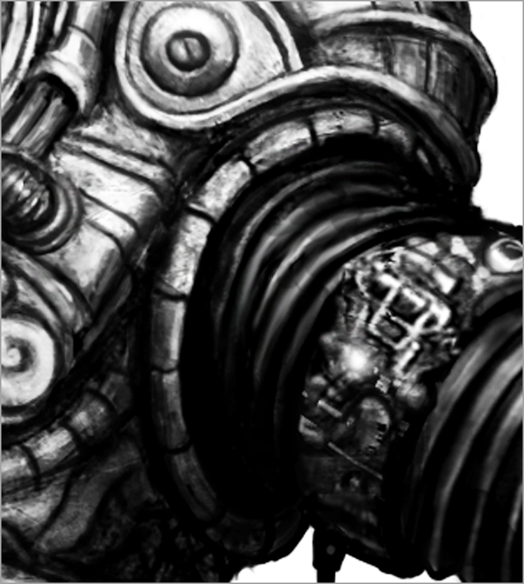
The example used in this chapter is based on a design created by Chris Sanchez. For this book, we asked Chris to design a character in a futuristic space suit that is heavily detailed and stylized in the hope that as many modeling techniques as possible could be demonstrated using a single project. Figure 3-16 shows Chris’s concept drawing.
Chris Sanchez
Chris Sanchez is a Los Angeles–based concept artist, illustrator, and storyboard artist. He attained his BFA in illustration from the Ringling College of Art and Design. He has foundations in traditional and digital techniques of drawing and painting. Chris has contributed designs to numerous film projects, including
Spider-Man 3,
Iron Man,
Iron Man 2,
Sherlock Holmes,
The Hulk,
Bridge to Terabithia,
RocknRolla, and
Tropic Thunder. For more of Chris’s work, visit
www.chrissanchezart.com.
It’s not unusual in the fast-paced world of production to be faced with building a model based on a single view of the subject. You’re also just as likely to be instructed to blend together several different designs. You can safely assume that the concept drawing you are given has been approved by the director. It’s your responsibility to follow the spirit of that design as closely as possible with an understanding that the technical aspects of animating and rendering the model may force you to make some adjustments. Some design aspects that work well in a two-dimensional drawing don’t always work as well when translated into a three-dimensional model.
The best way to start is to create some orthographic drawings based on the sketch. You can use these as a guide in Maya to ensure that the placement of the model’s parts and the proportions is consistent. Sometimes the concept artist creates these drawings for you; sometimes you need to create them yourself. (And sometimes you may be both modeler and concept artist.) When creating the drawings, it’s usually a good idea to focus on the major forms, creating bold lines and leaving out most of the details. A heavily detailed drawing can get confusing when working in Maya. You can always refer to the original concept drawing as a guide for the details. Since there is only one view of the design, some parts of the model need to be invented for the three-dimensional version. Figure 3-17 shows the orthographic drawings for this project.
After you create the orthographic drawings, your first task is to bring them into Maya and apply them to image planes.
Image planes are often used as a modeling guide. They are attached to the cameras in Maya and have a number of settings that you can adjust to fit your own preferred style.
1. Create a new scene in Maya.
2. Switch to the Side view. From the View menu in the viewport panel, choose Image Plane ⇒ Import Image (see
Figure 3-18).
3. A dialog box will open; browse the file directory on your computer, and choose the
spaceGirlSide.tif image from the
chapter3sourceimages directory at the book’s web page (
www.sybex.com/go/masteringmaya2014).
4. The side-view image opens and appears in the viewport. Select the sideShape in the Outliner, and open the Attribute Editor.
6. In the Image Plane Attributes section, you’ll find controls that change the appearance of the plane in the camera view. Make sure the Display option is set to In All Views. This way, when you switch to the perspective view, the plane will still be visible.
You can set the Display mode to RGB if you want just color, or to RGBA to see color and alpha. The RGBA option is more useful when the image plane has an alpha channel, and it is intended to be used as a backdrop in a rendered image as opposed to a modeling guide. There are other options, such as Luminance, Outline, and None.
The Color Gain and Color Offset sliders can be used to change the brightness and contrast. By lowering the Color Gain and raising the Color Offset, you can get a dimmer image with less contrast.
7. The Alpha Gain slider adds some transparency to the image display. Lower this slider to reduce the opacity of the plane.
Arranging Image Planes
In this example, the image plane is attached to the side-view camera in Maya, but you may prefer to create a second side-view camera of your own and attach the image plane to that. It depends on your own preference. Image planes can be created for any type of camera. In some cases, a truly complex design may require creating orthographic cameras at different angles in the scene.
If you want to have the concept drawing or other reference images available in the Maya interface, you can create a new camera and attach an image plane using the reference image (you can use the spaceGirlConcept.tif file in the chapter3sourceimages directory at the book’s web page). Then set the options so that the reference appears only in the viewing camera. Every time you want to refer to the reference, you can switch to this camera, which saves you the trouble of having the image open in another application.
8. When modeling, you’ll want to set Image Plane to Fixed so that the image plane does not move when you change the position of the camera. When using the image plane as a renderable backdrop, you may want to have the image attached to the camera.
Other options include using a texture or an image sequence. An image sequence may be useful when you are matching animated models to footage.
9. Scroll down in the Attribute Editor for the image plane. Under the Placement Extras rollout, you can use the Coverage sliders to stretch the image. The Center options allow you to offset the position of the plane in X, Y, and Z. The Height and Width fields allow you to resize the plane itself. In the Center options, set the Z field to -1.8 to slide the plane back a little.
10. Switch to the front camera, and use the View menu in the viewport to add another image plane.
11. Import the spaceGirlFront.tif image.
12. By default both image planes are placed at the center of the grid. To make modeling a little easier, choose the image plane shape nodes and move the images away from the center. Use the following settings:
Image Center X-attribute of the side-view image (imagePlaneShape1): -15
Image Center Z-attribute of the front-view image (imagePlaneShape2): -12
In the perspective view, you’ll see that the image planes are no longer in the middle of the grid (see
Figure 3-20).
Modeling NURBS Surfaces
To start the model of the space-suit character, begin by creating the helmet from a simple NURBS sphere:
1. Continue with the scene from the previous section, or open the spaceGirl_v01.ma scene from the chapter3scenes folder at the book’s web page. Make sure the images are visible on the image planes. You can find the source files for these images in the chapter3sourceimages folder.
2. Make sure you are on the Surfaces menu set. Choose Create ⇒ NURBS Primitives ⇒ Sphere to create a sphere at the origin. If you have Interactive Creation active in the NURBS Primitives menu, you will be prompted to draw the sphere on the grid. (I find Interactive Creation a bit of a nuisance and usually disable it).
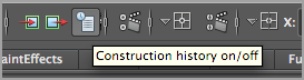
3. In the Channel Box for the sphere, click the makeNurbSphere1 node. If this node is not visible in the Channel Box, you need to enable the construction history and remake the sphere (on the status bar click the icon that looks like a script, as shown in
Figure 3-21). The construction history needs to be on for this lesson. Make sure Sections is set to
8 and Spans is set to
4. Set the Radius value to
1.0.
4. Switch to the side view, select the sphere, and move it up along the y-axis so it roughly matches the shape of the helmet in the side view (see
Figure 3-22). Enter the following settings in the Channel Box:
Translate X: 0
Translate Y: 9.76
Translate Z: 0.845
Rotate X: 102
Rotate Y: 0
Rotate Z: 0
Scale X: 2.547
Scale Y: 2.547
Scale Z: 2.547
5. To see the sphere and the reference, you can enable X-Ray mode in the side view (Shading ⇒ X-Ray). Also enable Wireframe On Shaded so that you can see where the divisions are on the sphere.
Artistic Judgment
Keep in mind that the main goal of this segment of the chapter is to give you an understanding of common NURBS modeling techniques. Creating a perfect representation of the concept image or an exact duplicate of the example model is not as important as gaining an understanding of working with NURBS. In some cases, the exact settings used in the example are given; in most cases, the instructions are general.
In the real world, you would use your own artistic judgment when creating a model based on a drawing; there’s no reason why you can’t do the same while working through this chapter. Feel free to experiment as you work to improve your understanding of the NURBS modeling toolset. If you want to know exactly how the example model was created, take a look at the scene files used in this chapter and compare them with your own progress.
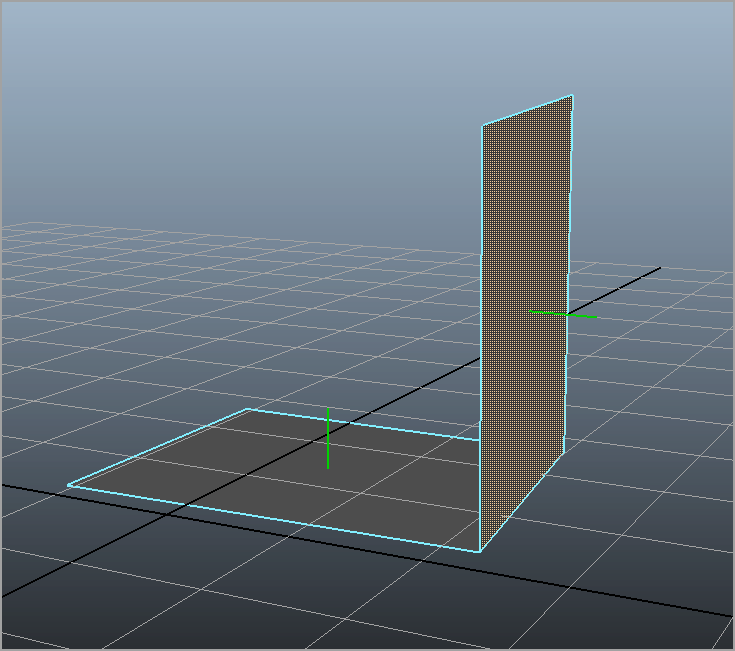
To create a separate surface for the glass shield at the front of the helmet, you can split the surface into two parts.
6. Right-click the sphere, and choose Isoparm. An isoparm is a row of vertices on the surface; sometimes it’s also referred to as knots.
7. Select the center line that runs vertically along the middle of the sphere.
8. Drag the isoparm forward on the surface of the sphere until it matches the dividing line between the shield and the helmet in the drawing (see
Figure 3-23).
9. Choose Edit NURBS ⇒ Detach Surfaces. This splits the surface into two parts along the selected isoparm. Notice the newly created node in the Outliner.
10. Rename detachedSurface1 as
shield, as shown in
Figure 3-24.
11. Select the shield, and scale down and reposition it so that it matches the drawing. Enter the following settings in the Channel Box:
Translate X: 0
Translate Y: 9.678
Translate Z: 1.245
Rotate X: 102
Rotate Y: 0
Rotate Z: 0
Scale X: 2.124
Scale Y: 2.124
Scale Z: 2.124
12. Right-click the rear part of the nurbsSphere1, and choose Control Vertex.
13. You’ll see the CVs of the helmet highlighted. Drag a selection marquee over the vertices on the back, and switch to the Move tool (hot key = w).
14. Use the Move tool to position these vertices so that they match the contour of the back of the helmet.
15. Select the Scale tool (hot key = r), and scale them down by dragging on the blue handle of the Scale tool.
16. Adjust their position with the Move tool so that the back of the helmet comes to a rounded point (see the top image in
Figure 3-25).
17. Select the group of vertices at the top of the helmet toward the back (the third isoparm from the left), and use the Move tool to move them upward so that they match the contour of the helmet (see the middle image in
Figure 3-25).
18. Select the group of vertices at the bottom of the helmet along the same isoparm.
19. Move these upward to roughly match the drawing (see the bottom image in
Figure 3-25).
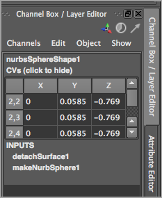
NURBS Component Coordinates
When you select CVs on a NURBS surface, you’ll see a node in the Channel Box labeled CVs (Click To Show). When you click this, you’ll get a small version of the Component Editor in the Channel Box that displays the position of the CVs in local space—this is now labeled CVs (Click To Hide)—relative to the rest of the sphere. The CVs are labeled by number. Notice also that moving them up in world space actually changes their position along the z-axis in local space. This makes sense when you remember that the original sphere was rotated to match the drawing.
20. Rename the back portion helmet.
21. Save the scene as helmet_v01.ma.
To see a version of the scene to this point, open the helmet_v01.ma scene from the chapter3scenes directory at the book’s web page.
Lofting Surfaces
A loft creates a surface across two or more selected curves. It’s a great tool for filling gaps between surfaces or developing a new surface from a series of curves. In this section, you’ll bridge the gap between the helmet and shield by lofting a surface:
1. Continue with the scene from the previous section, or open the helmet_v01.ma scene from the chapter3scenes folder at the book’s web page.
2. Switch to the side view; right-click the helmet surface, and choose Isoparm.
3. Select the isoparm at the open edge of the surface.
Selecting NURBS Edges
When selecting the isoparm at the edge of a surface, it may be easier to select an isoparm on the surface and drag toward the edge until it stops. This ensures that you have the isoparm at the very edge of the surface selected.
4. Right-click the shield, and choose Isoparm.
5. Hold down the Shift key, and select the isoparm at the edge of the surface so that you have a total of two isoparms selected: one at the open edge of the helmet and the other at the open edge of the shield (sometimes doing so takes a little practice).
6. Choose Surfaces ⇒ Loft ⇒ Options.
7. In the Loft Options dialog box, choose Edit ⇒ Reset Settings to set the options to the default settings.
8. Set Surface Degree to Linear and Section Spans to 5.
By setting Surface Degree to Linear, you can create the hard-edge ridge detail along the helmet’s seal depicted in the original drawing.
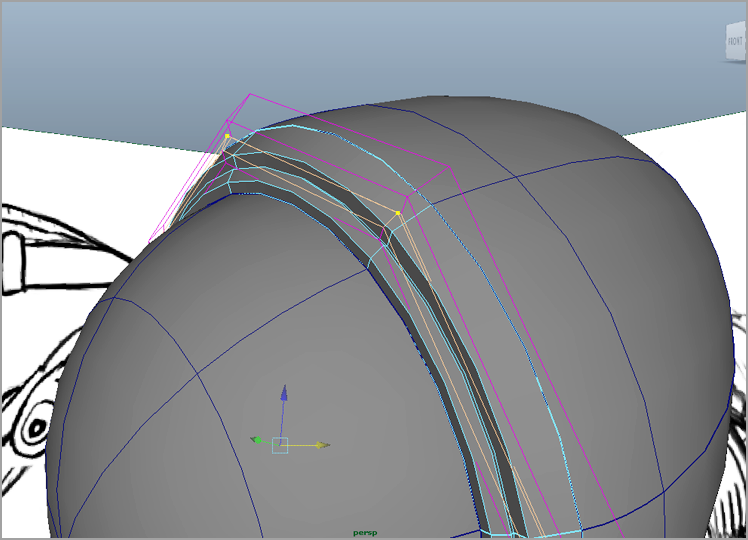
10. In the side view, zoom in closely to the top half of the loft.
11. Right-click the Loft, and choose Hull.
12. Select the second hull from the left, and choose the Move tool (hot key = w).
13. Open the options for the Move tool, and set Move Axis to Normals Average so that you can easily move the hull back and forth relative to the rotation of the helmet.
14. Move the hull forward until it meets the edge of the shield (see
Figure 3-27).
15. Using the up arrow key, select the next hull in from the left.
16. Move this hull toward the back to form a groove in the loft.
Pick Walking
Using the arrow keys to move between selected components or nodes is known aspick walking.
17. Use the Scale and Move tools to reposition the hulls of the loft to imitate some of the detail in the drawing.
18. Turn off the visibility of the image-plane layers, and disable X-Ray mode so that you can see how the changes to the loft look.
19. Switch to the perspective mode, and examine the helmet (see
Figure 3-28).
As long as the construction history is preserved on the loft, you can make changes to the helmet’s shape and the loft will automatically update. Upon close inspection, the original concept sketch looks as though the front of the helmet may not be perfectly circular. By making a few small changes to the helmet’s CVs, you can create a more stylish and interesting shape for the helmet’s shield.
20. Select the helmet and the shield but not the loft.
21. Switch to Component mode. The CVs of both the helmet and the shield should be visible.
22. Select the four CVs at the bottom center of the shield and the four CVs at the bottom of the helmet.
23. In the options for the Move tool, make sure Move Axis is still set to Normals Average.
24. Switch to the side view, and use the Move tool (hot key = w) to pull these forward toward the front of the helmet.
25. Switch to the Rotate tool (hot key = e), and drag upward on the red circle to rotate the CVs on their local x-axes.
26. Switch back to the Move tool, and push along the green arrow to move them backward slightly.
These changes will cause some distortion in the shape of the shield and the loft. You can adjust the position of some of the CVs very slightly to return the shield to its rounded shape.
27. Select the CVs from the side view by dragging a selection marquee around the CVs so that the matching CVs on the opposite side of the x-axis of the helmet are selected as well (as opposed to just clicking the CVs).
28. Use the Move tool to adjust the position of the selected CVs.
29. Keep selecting CVs, and use the Move tool to reposition them until the distortions in the surface are minimized. Remember, you are only selecting the CVs of the helmet and shield, not the CVs of the lofted surface in between (remember to save often!).
30. Save the scene as helmet_v02.ma.
This is the hardest part of NURBS modeling, and it does take practice, so be patient as you work. Figure 3-29 shows the process. Figure 3-30 shows the reshaped helmet and shield from the perspective view.
To see a version of the scene to this point, open the helmet_v02.ma scene from the chapter3scenes directory at the book’s web page.
Intersecting Surfaces
You can use one NURBS object to model another. Using a bit of ingenuity, you can find ways to create interesting shapes by carving a NURBS surface with a second surface. In this section, you’ll prepare the helmet in order to create an opening at its bottom so that the space-suit character can fit the helmet around her head:
1. Continue with the scene from the previous section, or open the helmet_v02.ma scene from the chapter3scenes directory at the book’s web page.
2. Create a new NURBS sphere with a radius of 1.0. Position the sphere so that it intersects the bottom of the helmet, and scale it in size so that it covers most of the bottom of the helmet. Use the following settings in the Channel Box:
Translate X: 0
Translate Y: 8.491
Translate Z: -1.174
Scale X: 1.926
Scale Y: 2.671
Scale Z: 2.834
3. Select the helmet, and then Shift+click the sphere.
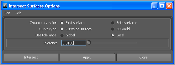
4. Choose Edit NURBS ⇒ Intersect Surfaces ⇒ Options.
5. In the Intersect Surfaces Options dialog box, choose Edit ⇒ Reset Settings to return the options to the default settings.
6. Set Create Curves For to First Surface. This creates a NURBS curve on the first selected surface.
7. Click the Intersect button to perform the operation (see
Figure 3-31).
8. In the viewport, you’ll see a new curve created on the helmet. Select the sphere you created for the intersection, and hide it (press Ctrl+h). You can see the curve drawn on the bottom of the helmet (see
Figure 3-32).
Because of the helmet’s construction history, if you move either sphere of the helmet, the curve will change positions. The curve on the surface can be selected and moved as well using the Move tool. As you reposition the curve on the surface, it will remain attached to the surface.
Trim Surfaces
When you trim a surface, you cut a hole in it. This does not actually delete parts of the surface; rather, it makes the parts invisible as if they had been deleted. This is one way to get around the fact that NURBS surfaces must consist of only four-cornered patches. To trim a surface, you must first create a curve on the surface, as demonstrated in the previous section:
1. Undo any changes made to the position of the two surfaces or the curve on the surface.
2. Select the helmet, and choose Edit NURBS ⇒ Trim Tool. When the Trim tool is activated, the surface appears as a white wireframe with the edges and curves on the surface highlighted in a bold solid line.
3. The Trim tool indicates which parts of the surface you want to remain visible when the Trim operation is completed. Use the tool to click several parts of the helmet, but not within the area defined by the curve on the surface.
4. Wherever you click, a marker indicates the parts of the surface that will remain visible. When you have created five or six markers, press the Enter key to trim the helmet. A hole will appear at the bottom of the helmet (see
Figure 3-33).
As with the curve on the surface, as long as the construction history is maintained for the surface, any changes you make to the intersecting spheres or the curve on the surface will change the position and shape of the hole in the helmet. You can animate the intersecting sphere to make the hole change size and shape over time; however, be aware that some changes may cause errors.
Working with Trim Edges
The edge of the trimmed surface can be used as a starting point for lofts or other NURBS surface types.
1. Right-click the helmet, and choose Trim Edge from the upper-left side marking menu. This option appears only for trimmed surfaces (see
Figure 3-34).
2. Select the trim edge (it should turn yellow when selected), and choose Edit Curves ⇒ Duplicate Surface Curves. Doing so creates a new curve that can be positioned away from the helmet.
3. Select the new curve, and choose Modify ⇒ Center Pivot so that the pivot point of the new curve is at its center.
4. Use the Move tool to position duplicateCurve1 below the helmet. Scale it up in size a little as well. Use these settings:
Translate X: 0
Translate Y: -0.174
Translate Z: 0
Scale X: 1.275
Scale Y: 1.275
Scale Z: 1.275
5. With the curve selected, tumble the view so that you can clearly see the bottom of the helmet.
6. Right-click the helmet, and choose Trim Edge.
7. Shift+click the trim edge at the bottom of the helmet so that both the duplicate curve and the trim edge are selected.
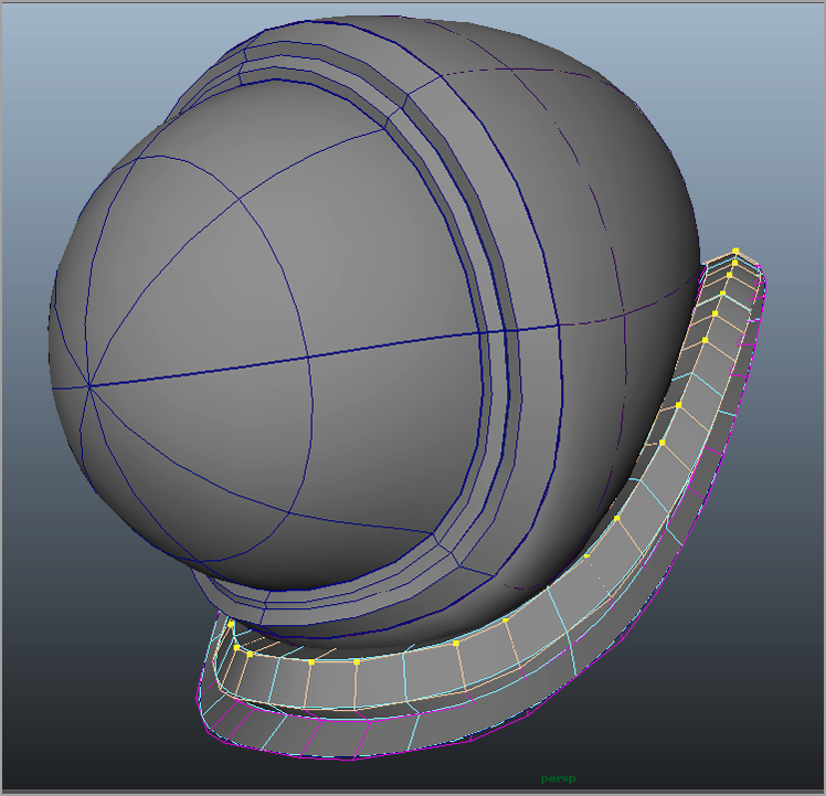
8. Choose Surfaces ⇒ Loft to create a loft using the same settings used to close the gap between the helmet and shield (see
Figure 3-35).
9. Right-click the new lofted surface, and choose Hull.
10. Use the Move and Scale tools to change the position and size of the hulls to create a couple of grooves in the loft. This technique is similar to the one used to add detail to the loft between the helmet and the shield (see
Figure 3-36).
11. Save the scene as helmet_v03.ma.
To see a version of the scene to this point, open the helmet_v03.ma scene from the chapter3scenes folder at the book’s web page.
Organizing Surfaces
When you’re working with NURBS surfaces, the Outliner can quickly fill up with oddly named objects, such as detachedSurface23. When the scene gets big, this can get confusing. To help reduce clutter and confusion, occasionally take the time to rename the surfaces as you’re working.
Fillet Surfaces
A fillet surface is another method for bridging gaps between surfaces. On top of the space suit’s helmet are two lamps. Using a fillet surface, you can bridge the gap between the lamp and its housing:
1. Open the helmet_v04.ma scene from the chapter3scenes directory at the book’s web page. The lamp and its housing have been added to the scene.
2. Select the isoparms at the edge of the reflector and the lamp housing.
3. From the Surfaces menu, choose Edit NURBS ⇒ Surface Fillet ⇒ Freeform Fillet.
4. The freeform fillet creates a smooth, rounded surface between the two surfaces. Select the freeformFiletSurface1 node, and open the Channel Box.
5. Set Depth to
0.8 and Bias to
-0.8. The Depth setting adjusts the curvature of the surface, and the Bias setting moves the influence of the curvature toward one end or the other of the fillet (see
Figure 3-37).
Next you’ll add some additional fillets to the lamp housing to create more detail.
6. Select the isoparms at both ends of the lamp housing. Choose Edit NURBS ⇒ Insert Isoparms ⇒ Options.
7. In the Insert Isoparms Options dialog box, set Insert Location to Between Selections, and set # Isoparms To Insert to 4.
8. Click the Insert button to make the change. This creates four new isoparms evenly spaced along the housing (see
Figure 3-38).
9. Select the four newly created isoparms, and choose Edit Curves ⇒ Duplicate Surface Curves.
10. Select the four curves, and center their pivots (Modify ⇒ Center Pivot).
11. Scale the curves up to 1.5 on the x- and y-axes.
12. Create two lofts between the two pairs of curves. Make sure the lofts are cubic, and give them both two section spans.
13. Create a freeform fillet by choosing an isoparm at the front edge of the front loft and an isoparm on the lamp housing just ahead of the loft.
14. Choose Edit NURBS ⇒ Surface Fillet ⇒ Freeform Fillet.
15. Perform steps 13 and 14 three more times to create fillets between the other edges of the two lofts and the lamp housing (see
Figure 3-39).
16. Right-click each loft, and choose Hulls. Shift+click the outside hulls on the top of both lofts, and use the Move tool to pull them upward.
17. Switch to the Scale tool, and scale them along the x-axis to flatten the tops of the lofts.
18. Shift+click the top-center hull on both lofts, and use the Move tool to pull them all down, closer to the housing.
19. Switch to the Rotate tool.
20. Rotate the hulls along the x-axis to give them a slight angle.
21. Experiment with the shape of these surfaces by continuing to translate, rotate, and scale the hulls of the lofted surfaces. Because of construction history, the freeform fillet surfaces will update. You can also make changes by editing the curves duplicated from the lamp housing isoparms in step 5.
Selecting and Moving Hulls
For some surfaces, selecting hulls can be tricky. If you’re having trouble selecting a specific hull, try selecting a nearby hull that is more exposed, and then use the arrow keys to pick walk your way to the hull you need to select.
22. Select all the surfaces that make up the lamp housing, the lofts, and the fillets.
23. Delete history on these surfaces, and group them. Name the group leftLamp (it’s on the character’s left).
24. Delete all the associated curves (see
Figure 3-40).
25. Select the leftLamp group, and choose Edit ⇒ Duplicate Special ⇒ Options.
26. In the Duplicate Special Options dialog box, set the Scale X to -1.
27. Click the Duplicate Special button. This creates a copy of the lamp on the opposite side of the helmet. Name the duplicate lamp group
rightLamp (see
Figure 3-41).
28. Save the scene as helmet_v05.ma.
To see the scene up to this point, open the helmet_v05.ma scene from the chapter3scenes directory at the book’s web page.
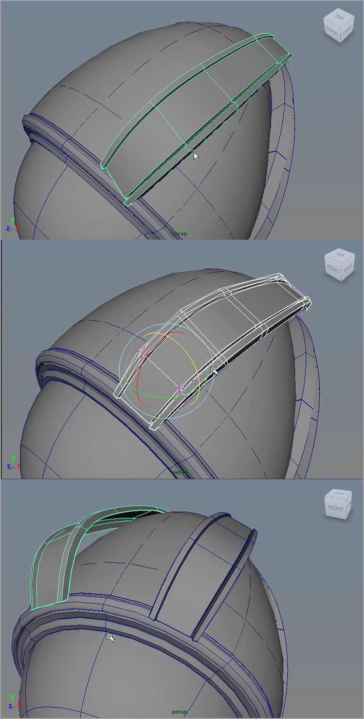
Creating Rail Surfaces
A rail surface uses at least one profile curve and two rail curves to create a surface.
1. Continue with the scene from the previous section, or open the helmet_v05.ma scene from the chapter3scenes directory at the book’s web page.
2. Select the leftLamp and rightLamp groups, and hide them (press Ctrl+h).
3. Switch to the side-view camera.
4. Switch to wireframe mode (hot key = 4).
5. Choose Create ⇒ CV Curve Tool (make sure you are in the side view).
6. Place the first point of the curve near the front/top of the helmet.
8. Switch to the front view.
9. Select the curve, and choose Modify ⇒ Center Pivot.
10. Select the Move tool.
11. Press and hold the d key on the keyboard to switch to pivot mode. You can also press the Insert key without holding it, to switch to pivot mode.
12. Pull down on the y-axis of the Move tool.
13. Reposition the pivot so that, from the front view, it is aligned with the center of the helmet’s shield (see
Figure 3-43). Once you move the pivot, you can let go of the d key or press the Insert key again to return to the normal transformation mode.
14. Switch to the Rotate tool (hot key = e).
15. Rotate the curve -14 degrees on the z-axis.
16. Duplicate the curve (press Ctrl/Cmd+d), and rotate the duplicate -29 degrees on the z-axis.
17. Scale the duplicate curve to 0.95 on the y-axis. These two curves will become the rails for the birail surface.
18. Switch to the perspective view, and turn Shading Mode back on.
19. Turn on Curve Snapping or hold down the c key, and select the EP Curve tool (Create ⇒ EP Curve Tool). This will allow you to create a curve by clicking just twice.
20. Click the first rail curve, and drag toward the end to make the first point of the curve.
21. Click the second rail curve and drag toward its end (toward the back of the helmet) to make the second point of the curve. This might be easier to do if you rotate the view so that the curves are not overlapping the surfaces. This helps avoid a situation in which Curve Snapping places one of the points of the EP curve on one of the isoparms of a visible surface (see
Figure 3-44).
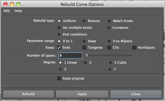
22. Select the curve between the two rails, and choose Edit Curves ⇒ Rebuild Curve ⇒ Options.
23. In the Rebuild Curve Options dialog box, reset the settings. Set the following:
Number Of Spans: 8
Degree: 1 Linear
24. Click Rebuild to rebuild the curve (see
Figure 3-45).
25. Select the new curve, and switch to component mode.
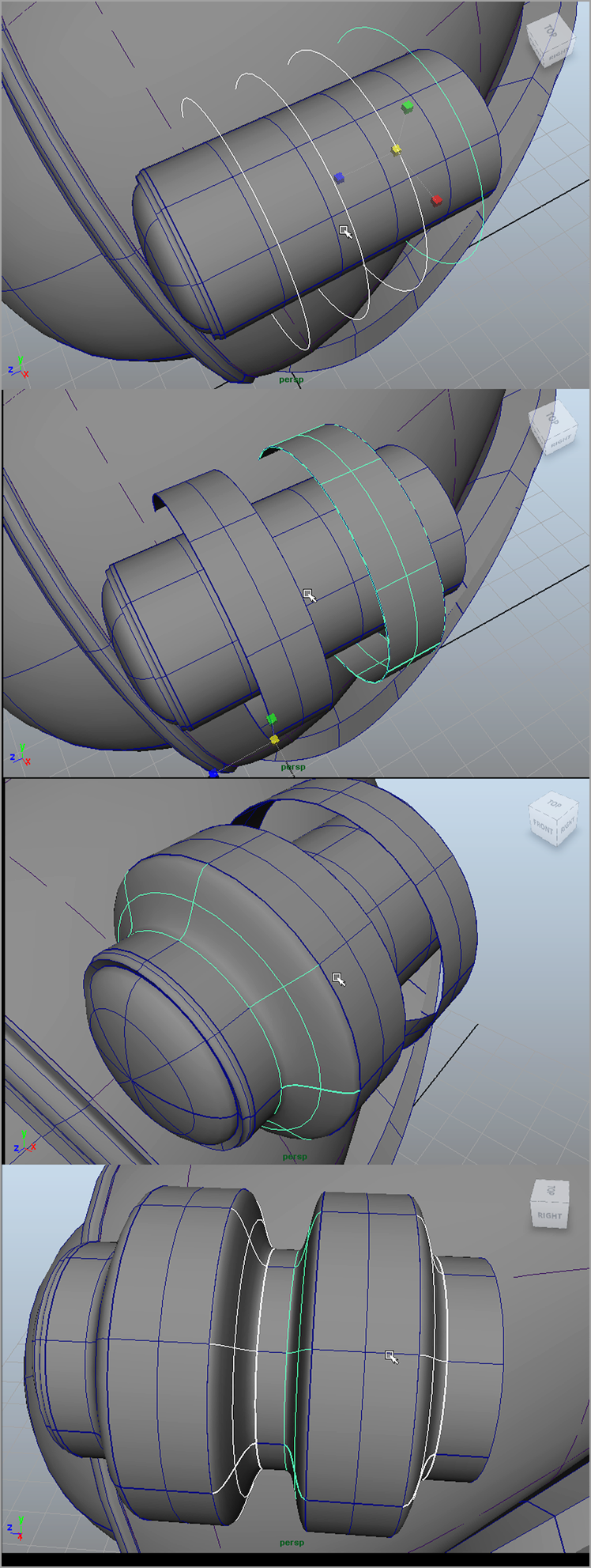
26. Turn Curve Snapping off. Use the Move tool to drag some of the CVs to shape the profile. The profile will be swept along the curves to create grooves, similar to the detail on the top of the helmet in the drawing. You can keep it simple for now and add detail later.
Moving CVs and Other Components
While using the Move tool to edit the position of CVs, experiment with the different axis settings in the Move tool options. Sometimes it’s easier to use object mode, whereas other times another mode is preferable. You can even use the position of a specific CV (or edge or face) to set the axis of the Move tool. To do so, switch the object to component mode, open the Move Tool Options box, click the Set To Point button, and then select a CV. The axis of the Move tool will be oriented to face the CV.
27. To create the birail, choose Surfaces ⇒ Birail ⇒ Birail1 Tool. (The options may open automatically; if they do, click the Birail 1 Tool button to start using the tool.)
28. In the viewport, select the profile curve first and press Enter.
29. Select the first and then the second rail curves. Press Enter (see
Figure 3-46).
You can change the shape of the surface by editing the position of the CVs on the profile curve. Be careful not to change the position of the rail curves. If the three curves no longer touch, the surface will disappear.
30. To make changes to the surface, select it, delete the history, and then edit the surface by selecting the hulls and moving them with the Move tool.
31. When you’re happy with the basic shape of the birail, select it and choose Edit ⇒ Duplicate Special ⇒ Options.
32. In the Duplicate Special Options dialog box, set Scale X to -1.
33. Click Duplicate Special. This makes a copy of the surface on the opposite side of the helmet (see
Figure 3-47).
34. Create a loft between the two inside edges of the birail surface. The loft should have nine divisions.
35. Use the Move tool to position the hulls of the loft to create the three curving bumps as shown in the concept sketch (see
Figure 3-48).
36. Select the surface, and choose Edit ⇒ Delete By Type ⇒ History to remove the construction history from the object.
37. Save the scene as helmet_v06.ma.
Lofting Across Multiple Curves
To create the back of the helmet, you can loft a surface across multiple profile curves:
1. Continue with the scene from the previous section or open the helmet_v06.ma scene from the chapter3scenes directory at the book’s web page.
2. Right-click the rear of the housing for the leftLamp; select Isoparm. Select the isoparm at the very back-end of the housing.
3. Choose Edit Curves ⇒ Duplicate Surface Curves to create a curve based on the selected isoparm.
4. Choose Edit ⇒ Duplicate Special ⇒ Options, and set Scale X to -1.
5. Click the Duplicate Special button to make a mirror copy of the curve on the other side.
6. Select the original curve, and choose Edit ⇒ Duplicate (or press Ctrl/Cmd+d) to make a standard duplicate of the curve.
7. Set the rotation of this curve to 50 degrees in Y.
8. Select the curve on the opposite side, and duplicate it as well. Set the Y-rotation to -50 degrees.
9. Starting from the helmet’s left side, Shift+click each of the duplicate curves. (This may be easier to do if you hide the NURBS surfaces using the Show menu in the panel menu bar.)
10. Choose Surfaces ⇒ Loft ⇒ Options. In the Loft Options dialog box, make sure the degree of the loft is set to Cubic. Set the Section Spans to 2.
11. Click the Loft button.
12. When the loft is created (turn the visibility of NURBS surfaces back on to see the loft), right-click the new surface, and choose Control Vertex to switch to component mode.
13. Select pairs of CVs at the back of the surface, and use the Move tool to reposition them to create a more interesting shape to the surface (see
Figure 3-49).
14. Name the new surface helmetRear. When you’re happy with the result, save the model as helmet_v07.ma.
To see a version of the scene to this point, open the helmet_v07.ma scene from the chapter3scenes directory at the book’s web page.
Live Surfaces
When you make a NURBS surface “live,” you put it into a temporary state that allows you to draw curves directly on it. This is a great way to add detail that conforms to the shape of the object.
1. Continue with the scene from the previous section, or open the helmet_v07.ma scene from the chapter3scenes directory at the book’s web page.
2. Make sure that Wireframe On Shaded is enabled, and zoom into the model so that you can see the birail surface you created in the previous section.
You’re going to add some isoparms to the surface so that drawing clean curves on the surface will be a little easier. The isoparms will act as a guide for the curves that you draw.
3. Right-click the birail surface, and choose Isoparm.
4. Add two isoparms that run along the length of the birail surface. (In the options for Insert Isoparm, make sure Location is set to At Selection.)
5. Add two additional isoparms just outside the isoparms created in step 4.
6. Add two additional isoparms that run across the surface, as shown in the bottom image in
Figure 3-50.
7. With the birail surface selected, choose Modify ⇒ Make Live to make the surface live. You’ll see that the wireframe lines now appear green on the surface.
8. Enable Snap To Grids, and choose Create ⇒ CV Curve Tool ⇒ Options.
9. In the Tool Settings dialog box, make sure Curve Degree is set to 1 Linear.
10. With Snap To Grids enabled, the points of the curve will be snapped to the isoparms on the surface. Follow the guide in
Figure 3-51 to add points to the curve.
11. Finish the curve by clicking one more time at the point where you started the curve. When you are finished, press Enter.
12. Repeat steps 10 and 11 to add another curve that surrounds the first. Make sure that you add the same number of points in the same order and that you close the curve when finished.
13. To select curves on a surface, turn off Surface Selection in the Selection Mask Options and select the curves drawn on the surface.
14. Select the outside curve, and then Shift+click the inside curve.
15. Choose Surfaces ⇒ Loft ⇒ Options.
16. In the Loft Options dialog box, make sure the degree of the loft is Cubic and the number of section spans is set to 2.
17. Click Loft to make the loft.
18. When the loft is created, right-click it and choose Hulls.
19. Turn off Snap To Grids, and select the three central hulls of the loft. Switch to the Move tool.
20. In the Tool Settings dialog box, set the Move Axis to Normals Average and pull the hull up to create a raised surface (see
Figure 3-52).
21. To make the birail surface “unlive,” choose Modify ⇒ Make Live. You can only have one “live” surface at a time. If you have a new object selected while making the previous selected object “unlive,” the new selected object will become “live.”
Construction History
As long as the Construction History option for the loft surface is enabled, you can experiment with the position of the loft by selecting the curves on the surface and moving them around using the Move tool.
Figure 3-53 shows the completed NURBS helmet from different views. Open the NURBShelmet.ma scene from the chapter3scene directory at the book’s web page and examine the model to see whether you can figure out the techniques that were used to make it. All of the techniques used are just variations of the ones described in this section.
Mirror Objects
When you’ve completed changes on one side of the model, you can mirror them to the other side:
1. Create a group for the parts you want to mirror; by default, the pivot for the new group will be at the center of the grid.
2. Select the group and choose Edit ⇒ Duplicate Special.
3. Set Scale X of the duplicate to -1.
When you create the duplicate, you can freeze transformations on the objects and ungroup them if you like.
NURBS Tessellation
While working with NURBS surfaces, you may see small gaps or areas around the trim edge that do not precisely follow the curve. This is due to the settings found in the NURBS Display section of the surface’s Attribute Editor. These settings adjust how the NURBS surfaces appear while working in Maya. They do not necessarily represent how the object will look when rendered. By increasing the precision of the NURBS surface display, you may find that the performance of Maya on your machine suffers. It depends on the amount of RAM and your machine’s processor speed. The main thing to remember is that changing these settings will not affect how the surface looks when rendered.
To preview how the surface will look in the render, you can enable Display Render Tessellation in the Tessellation rollout of the surface’s Attribute Editor. A wireframe will appear on the surface, which represents the arrangement of triangles that will be used when the surface is converted to polygons by the renderer. (Note that the surface will remain as NURBS in the scene when you render.)
Using the Tessellation settings found in the Simple or Advanced Tessellation Options, you can determine how the surface will look when rendered (see Figure 3-54). Keep in mind that increasing the precision of the tessellation will increase your render time. You can adjust the settings based on how close an object is to the rendering camera. The triangle count gives you precise numeric feedback on how many triangles a surface will contain based on its tessellation settings. Take a look at the NURBSdisplay.ma scene in the chapter3scenes directory at the book’s web page.
The Advanced Tessellation settings give you even more control over how the object will be tessellated. In some circumstances, you may get better results using Simple Tessellation rather than Advanced. It depends on the model and the scene. If you’re having problems with the scene, you can experiment using the two methods.
Modeling with Polygons
Maya 2014 introduces the Modeling Toolkit. This kit provides easy access to commonly used functions and tools for polygon manipulation. You can open the toolkit by clicking its tab, on the right side of the screen, below the Channel Box tab. A power button–style icon at the top of the toolkit allows you to activate or deactivate the toolkit. When the toolkit is active, the Tool Settings window becomes inactive and can be closed to free more screen space in your work area. Likewise, when you choose a specific tool from the Tool Box the Modeling Toolkit becomes inactive.
To make the torso for the space-suit character, you’ll start with a technique known as box modeling. This technique uses the polygon-modeling tools to shape a basic cube into a more complex object. Once the form is established, you can add more geometry to create detail.
Shaping Using Smooth Mesh Polygon Geometry
In this section, you’ll create the basic shape of the torso for the space-suit character using smooth mesh polygon geometry:
1. Open the torso_v01.ma scene from the chapter3scenes directory at the book’s web page.
In this scene, you’ll see the NURBS helmet as well as the image planes that display the reference images.
2. Choose Create ⇒ Polygon Primitives ⇒ Cube using the default creation options.
3. Switch to a side view and turn on X-Ray mode (Shading ⇒ X-Ray) so that you can see the reference images through the geometry.
4. Select the cube, and name it torso. Position and scale the torso so that it roughly matches the position of the torso in the side view.
5. Set the channels as follows:
Translate X: 0
Translate Y: 6.375
Translate Z: -1.2
Scale X: 8.189
Scale Y: 6.962
Scale Z: 6.752
6. In the Channel Box, click the polyCube1 heading in the INPUTS section. Set Subdivisions Width to
4 and Subdivisions Height and Depth to
3, as shown in
Figure 3-55.
7. With the torso selected, press the 3key to switch to smooth mesh preview. The edges of the cube become rounded.
Smooth Mesh Preview Settings
By default, the smooth mesh preview displays the smoothing at two divisions, as if you had applied a smoothing operation to the geometry twice. You can change the display settings on a particular piece of polygon geometry by selecting the object and choosing Display ⇒ Polygons ⇒ Custom Polygon Display. At the bottom of the Custom Polygon Display Options dialog box, you’ll find the Smooth Mesh Preview settings. Changing the value of the Division Levels slider sets the number of subdivisions for the smooth mesh preview. You can also enable the Show Subdivisions option to see the subdivisions on the preview displayed as dotted lines. The options are applied to the selected object when you click the Apply button. Be aware that a high Division Levels setting slows down the performance of playback in Maya scenes.
Additional controls are available under the Extra Controls rollout. Lowering the Continuity slider decreases the roundness of the edges on the preview. You can also choose to smooth the UV Texture coordinates and preserve Hard Edges and Geometry borders.
8. Open the Modeling Toolkit by clicking the vertical tab on the right side of the screen. Choose the Move Tool (see
Figure 3-56). Clicking on any of the transformation tools automatically activates the toolkit. It also sets your component selection to Multi-Component mode.
9. Under the Transformations rollout change the coordinate space from World to Local. Expand the Soft Select rollout, directly under the Transformations rollout, and check Soft Selection. Set the falloff value to
3 (see
Figure 3-57).
10. The Modeling Toolkit has a symmetry function allowing you to work on half of the model while the other half automatically updates. To activate symmetry you select a single edge.
Enable Reflection; the default Reflection setting should work.
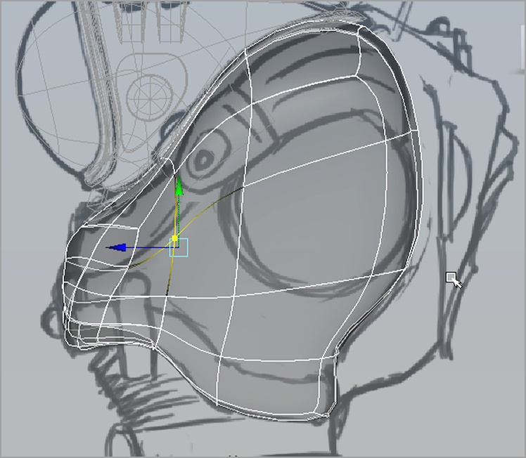
11. From the side view, select vertices and use the Move tool to reposition the vertices of the torso to roughly match the sketch. The torso surface will serve as a frame for the upper part of the space suit. At this time, you want to keep the amount of detail fairly low.
12. Adjust the selection settings as you work. Align the four corners of one of the faces toward the rear with the arm-socket opening in the sketch, as shown in
Figure 3-58.
Smooth Mesh Vertex Display
As you select vertices using the Move tool, you’ll notice that the handle of the Move tool is offset from the selected vertices. If you find this confusing, press the 2 key to see a wireframe cage of the original mesh. Then you’ll see the actual positions of the vertices on the unsmoothed version of the surface.
13. Switch to the front view, and continue to shape the cube to roughly match the drawing. Remember, your goal is to create a rough shape at this point. Most of the details will be added as additional sections of armor later (see
Figure 3-59).
Since you’ve already shaped much of the profile in the side view, restrict the changes you make in the front view to movements along the x-axis.
14. Finally, switch to the perspective view, and shape the torso further. This requires some imagination and artistic judgment as to how the shape of the space suit looks in perspective. It may be easier to do this if you turn off X-Ray mode and set the helmet display layer to Template mode.
Remember to refer to the original sketch; if you switch to the referenceImage camera, you’ll see the sketch on an image plane. Also remember to adjust your Move tool selection settings as needed. Always keep things as simple as possible, and avoid getting lost in the details.
15. Save the scene as torso_v02.ma.
To see a version of the scene to this point, open the torso_v02.ma scene from the chapter3scenes directory at the book’s web page.
Tweak Mode
You can activate tweak mode for the Move tool by choosing Tweak/Marquee from the Modeling Toolkit. This option is located under the Move tool icon at the top of the toolkit. When this is on, any component you touch is nudged in the direction of the mouse-pointer movement. Combined with Soft Select, the Move tool feels much more like a sculpting tool, and changes are more intuitive. Note that the Move tool manipulator is not displayed when tweak mode is activated.
Insert Edge Loops
An edge loop is an unbroken ring of edges that traverses polygon geometry, similar to an isoparm in NURBS geometry. Think of the circular areas around your lips and eyes. In 3D modeling, these areas are often defined using edge loops. You can insert edge loops into a model interactively using the Insert Edge Loops tool:
1. Continue with the scene from the previous section, or open the torso_v02.ma scene from the chapter3scenes directory at the book’s web page.
2. Select the Polygons menu set from the upper-left menu in the interface.
3. Switch to the side view.
4. Select the torso object, and choose Edit Mesh ⇒ Insert Edge Loop Tool. The wireframe cage appears around the torso while the tool is active.
Custom Toolkit Buttons
The Insert Edge Loop tool is not included as part of Modeling Toolkit Mesh Editing Tools. You can add it however to the Custom Shelf section located at the bottom of the toolkit. To add a tool, choose it through its normal menu. Once the tool has been used, its icon is displayed in the Last Tool Used square of the toolbox. MMB-drag the icon to the Custom Shelf of the toolkit.
5. Click one of the cage’s edges at the bottom row of the torso, as shown in
Figure 3-60.
Edge loops are always added perpendicular to the selected edge. The loop continues to divide polygons along the path of faces until it encounters a three-sided or
n-sided polygon (see
Figure 3-61).
6. Once you have inserted the edge loop, press q to drop the tool. (As long as the tool is active, you can continue to insert edge loops in a surface.)
7. Select the edge loop, if it is not already selected, by double-clicking on one of the loop’s edges. Choose Edit Mesh ⇒ Edit Edge Flow.
8. Click on polyEditEdgeFlow1 in the Channel Box. Click on Adjust Edge Flow, and then MMB in the viewport to adjust the shape of the inserted edge loop.
The Edit Edge Flow tool allows you to shape edge loops to better fit or respect the surrounding surface. You can choose as many loops as you want; however, the results tend to blend together, flattening the surface. Stick to one or two loops. The Edit Edge Flow options are also available through the Insert Edge Loop and Offset Edge Loop tools. However, you cannot use the Edit Edge Flow option when inserting multiple edges.
9. Continue to shape the torso using the edge flow options and vertex manipulation with the Move tool (see
Figure 3-62).
10. Save the scene as torso_v03.ma.
To see a version of the scene to this point, open the torso_v03.ma scene from the chapter3scenes directory at the book’s web page.
Be Stingy with Your Edge Loops
It’s always tempting to add a lot of divisions to a surface to have more vertices available for sculpting detail. However, this often leads to a confusing and disorganized modeling process. Keep the number of vertices in your meshes as low as possible. Add only exactly what you need, when you need it. If you are disciplined about keeping your models simple, you’ll find the modeling process much easier and more enjoyable. Too many vertices too early in the process will make you feel like you’re sculpting with bubblegum.
Extruding Polygons
Extruding a polygon face adds geometry to a surface by creating an offset between the extruded edge or face. New polygon faces are then automatically added to fill the gap between the extruded edge or face. In this section, you’ll see a couple of the ways to use extrusions to shape the torso of the space suit:
1. Continue with the scene from the previous section, or open the torso_v03.ma scene from the chapter3scenes directory at the book’s web page.
2. Switch to the perspective view, and turn off X-Ray Shading.
3. Right-click the model, and choose Face to switch to face selection mode.
4. Select the face on the side that corresponds with the placement of the arm socket. Shift+click the matching face on the opposite side.
5. Choose Edit Mesh ⇒ Extrude or select it from the Modeling Toolkit. A manipulator appears at the position of the new extruded face along with three input values controlling the Thickness, Offset, and Divisions attributes. If you chose Extrude from the toolkit, the manipulator is not displayed. The options open in a new rollout below the Mesh Editing Toolkit.
Input Extrude Values
The input fields allow you to use any value, positive or negative, for the Thickness and Offset attributes. The input field also obeys the precision set through the Channel Box using Edit ⇒ Settings ⇒ Change Precision.
6. Click and drag the blue arrow of the manipulator to move the extruded face toward the center of the torso. The extruded face on the opposite side should move into the center as well.
7. Change the Divisions to
2 by typing the value into the floating input. This increases the number of polygons used to bridge the gap between the extruded face at the torso (see
Figure 3-63). You can also MMB-drag left or right to change the input. Holding Shift increases the input speed, whereas Ctrl decreases the speed.
8. Select the six faces on the top of the torso that are directly beneath the NURBS helmet. It’s a good idea to turn on Camera Based Selection in the Select Tool options. This prevents you from accidentally selecting faces on the opposite side of the torso. You can also turn off Soft Select.
9. Choose Edit Mesh ⇒ Extrude.
10. Click one of the scale cubes at the end of the manipulator handle (at the tip of one of the arrows). This switches the manipulator to scale mode.
11. Drag to the left on the light blue cube at the center of the manipulator to scale down the extruded faces.
12. Set the Divisions value to 2.
13. Drag the blue arrow of the extrude manipulator downward to create a depression at the top of the torso (see
Figure 3-64).
14. Turn Soft Select on, and use the Move tool to shape the torso so that it matches the design on the image planes. The base of the helmet should stay on top of the torso (see
Figure 3-65).
15. Save the scene as torso_v04.ma.
To see a version of the scene to this point, open the torso_v04.ma scene from the chapter3scenes directory at the book’s web page.
Edge Creasing
One drawback to using the smooth mesh preview on polygon objects is that surfaces can look too smooth and almost pillow-like. To add hardness to the edges of a smoothed object, you can use creasing.
In this section, you’ll create the arm-socket detail so that you have a place to insert the arms into the torso (see Figure 3-66):
1. Continue with the scene from the previous section, or open the torso_v04.ma scene from the chapter3scenes directory at the book’s web page.
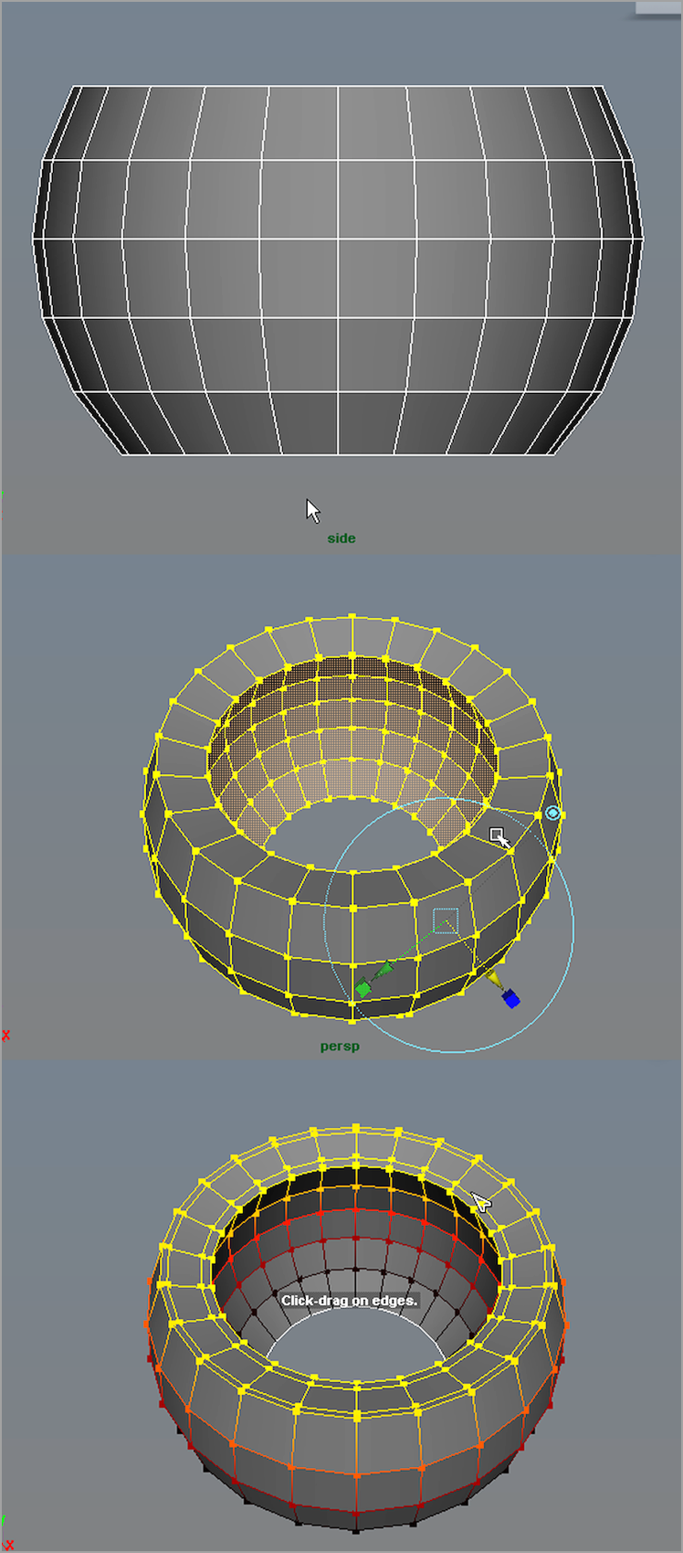
2. Create a polygon sphere (Create ⇒ Polygon Primitives ⇒ Sphere).
3. In the INPUTS section of the Channel Box, set Subdivisions Axis to 24 and Subdivisions Height to 12.
4. Switch to a side view, and zoom in on the sphere.
5. Right-click the sphere, and choose Face.
6. In the Tool Settings dialog box, set Selection Style to Marquee. Turn off Camera Based Selection and Soft Select.
7. Select the top four rows on the sphere and delete them.
8. Select the bottom three rows on the sphere and delete them as well.
9. Switch to the perspective view. Select the sphere, and name it socket.
10. With socket selected, choose Edit Mesh ⇒ Extrude. This extrudes all the faces at the same time. Change the Thickness to -0.2.
11. Change the Divisions to 3.0.
12. Double-click a single edge from the outer division loop you added. The entire loop is selected.
13. Use Edit Mesh ⇒ Slide Edge Tool to push the edge loop out further. It should snap into place automatically using the default snapping settings of the Slide Edge tool. Repeat the process for the inner loop, as shown in the third image of
Figure 3-67.
14. Rotate the view so that you can clearly see the top of the socket.
15. Select the middle row of polygon faces around the top. You can select the entire row by choosing a face and then holding Shift and double-clicking an adjacent face.
Deselecting Polygons
If you select extra polygons by accident, you can hold the Ctrl key and paint on them to deselect them. To add to the current selection, hold the Shift key while painting the selection.
16. With the faces selected, choose Edit Mesh ⇒ Extrude.
17. Open the Channel Box for the polyExtrudeFace4 node.
18. Toward the bottom, set Keep Faces Together to off.
19. Click one of the scale cubes at the tip of the arrows on the Extrude manipulator to switch to scale mode.
20. Drag the light blue cube at the center of the manipulator to scale down the extruded faces. Note that with Keep Faces Together turned off, each face is extruded individually.
21. With faces selected, create another extrusion (the g hot key repeats the last action).
22. Enter a value of -.06 for the Thickness.
23. When you have finished creating the extrusion, press the q hot key or choose another tool to deselect the Extrusion tool.
24. Select the socket object, and press the
3 key to switch to smooth mesh preview. The extrusions at the top look like rounded bumps (see
Figure 3-68).
25. Use the Select tool to select each of the faces at the top of the rounded bumps. Hold the Shift key as you select each face.
26. Once you have all the faces selected, press Shift + > to expand the selection one time. The faces around each bump are now selected as well.
27. Choose Select ⇒ Convert Selection ⇒ To Edges. Now the edges are selected instead of the faces.

28. The newly extruded faces appear rounded when using the smooth mesh preview. Using the crease tools, you can change the curvature of the edges. Open Edit Mesh ⇒ Crease Editor. The Crease Editor is new to Maya 2014. It allows you to make a set from your selection and adjust the hardness of the creased edges in a predictable manner.
29. Drag the Crease Editor to the right-hand side of the screen. The editor will automatically dock to the interface. Choose New from the top-left corner of the Crease Editor to make a set from your current selection. Use the default name of creaseSet1 for its name.
30. Click on creaseSet1 to highlight it. While in the Crease Editor, drag to the right while holding the MMB. The edges become less round as you drag to the right and rounder as you drag to the left. Set the creasing so that the edges of the bumps are just slightly rounded.
31. Select the socket object, and switch to Edge Selection mode.
32. Double-click the first edge loop outside the extruded bumps. Double-clicking an edge selects the entire edge loop.
33. Use the Crease Editor to create a crease set from the selected edge loop.
34. Repeat steps 31–33 for the first edge on the inside of the socket just beyond the extruded bumps. Add a crease to the edges (see
Figure 3-69).
35. Select the socket, and switch to the Move tool.
36. Move, scale, and rotate the socket so that it fits into the space on the side of the torso (see
Figure 3-70).
37. Set these values in the Channel Box:
Translate X: 3.712
Translate Y: 7.5
Translate Z: -2.706
Rotate X: 11.832
Rotate Y: 5.385
Rotate Z: -116.95
Scale X: 1.91
Scale Y: 1.91
Scale Z: 1.91
38. After placing the socket, spend a few minutes editing the position of the points on the torso so that the socket fits more naturally.
39. Save the scene as torso_v05.ma.
To see a version of the scene to this point, open the torso_v05.ma scene from the chapter3scenes directory at the book’s web page.
Crease Sets
If you create a crease for a number of selected edges that you will later readjust, you can create a crease set. A crease set saves the currently selected creased edges under a descriptive name. To create a crease set, follow these steps:
1. Select some edges that you want to crease or that already have a crease.
2. Choose Edit Mesh ⇒ Create Sets ⇒ Create Crease Set ⇒ Options.
3. In the options, enter a descriptive name for the set.
Any time you want to select the edges again to apply a crease, follow these steps:
1. Choose Edit Mesh ⇒ Crease Sets.
2. Choose the name of the set from the list.
The edges will then be selected, and you can apply or adjust the creasing as needed.
Mirror Cut
The Mirror Cut tool creates symmetry in a model across a specified axis. The tool creates a cutting plane. Any geometry on one side of the plane is duplicated onto the other side and simultaneously merged with the original geometry.
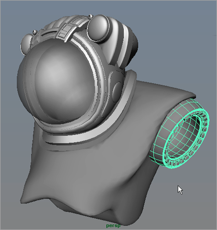
The back side of the shoulder armor is not visible in the image (see Figure 3-71), so we’re going to assume that it’s a mirror image of the geometry on the front side. You’ll model the front side first and then use Mirror Cut for the geometry across the z-axis to make the back.
In this section, you’ll model the geometry for the space suit’s shoulder armor. You’ll start by modeling the armor as a flat piece and then bend it into shape later.
In the options for Mirror Cut, you can raise the Tolerance, which will help prevent extra vertices from being created along the center line of the model. If you raise it too high, the vertices near the center may be collapsed. You may have to experiment to find the right setting.
1. Continue with the scene from the previous section, or open the torso_v05.ma scene from the chapter3scenes directory at the book’s web page.
2. Create a new display layer named TORSO.
3. Add the torso and the socket geometry to this layer, and turn off the visibility of the layer.
4. Turn off the visibility of the other layers as well so that you have a clear view of the grid.
5. Create a polygon pipe by choosing Create ⇒ Polygon Primitives ⇒ Pipe.
6. In the polyPipe1 node (under the INPUTS section of the Channel Box), use the following settings:
Radius: 1
Height: 1
Subdivisions Axis: 24
Subdivisions Caps: 2
7. Switch to the top view.
8. Choose the Move tool.
9. In the Tool Settings dialog box, set Selection Style to Marquee and turn off Camera Based Selection. This way you can select vertices on the top and bottom of the geometry from the top view.
10. Turn off Soft Select, and turn on Reflection. Make sure Reflection Axis is set to the x-axis.
11. Right-click the pipe, and choose Vertex.
12. Select the vertices on the outer edge of the pipe in the top half of the screen.
13. Use the Scale and Move tools to move them away from the pipe.
14. Scale them up so that the upper edge of the pipe has a shallow arc, as shown in the top image of
Figure 3-72.
15. Select the vertices on the outer edge of the pipe at the bottom of the screen.
16. Use the Move tool to shape these vertices so that they are slightly closer to the center. Use the bottom image in
Figure 3-70 as a reference.
17. Switch to the perspective view.
18. Turn on Marquee and Camera Based Selection in the Select Tool options.
19. Right-click the pipe, and choose Face. Select the faces at the wide end of the pipe, as shown in the first image in
Figure 3-73.
20. Choose Edit Mesh ⇒ Extrude to perform an extrusion on these faces. Before you move the extrusion with the manipulator, click the blue circle switch on the manipulator to extrude in world space (the second image in
Figure 3-73).
21. Pull the blue arrow of the manipulator to extend the face about three and a half units.
22. Use the blue scale handle of the Extrude manipulator to flatten the arc in these extruded faces.
23. Set the Divisions to 8.
24. Select the pipe, and choose Mesh ⇒ Mirror Cut. A plane appears at the center of the pipe.
25. In the Channel Box, set the Y-rotation of mirrorCutPlane1 to 0. The pipe is now mirrored across the z-axis.
26. Set the Translate Z channel of mirrorCutPlane1 to -3.42. The mirrored geometry is extended. If you see extra triangular polygons appearing near the cutting plane, try moving the plane back and forth a little until they disappear.
Disappearing Polygons
It may look as though polygons disappear when you use the Mirror Cut tool. It might just be that Maya is not displaying them correctly. If this happens to you, select the object and apply a Lambert shader to it. (Just switch to the Rendering shelf, and click the Lambert Material icon.) This should fix the problem.
In the Outliner, several new nodes have been created. These include the mirrorCutPlane1 and the mirroredCutMesh1 group. The pipe has been renamed polySurface1 (see
Figure 3-74).
27. Select the polySurface1 node, and choose Edit ⇒ Delete By Type ⇒ History. This removes the group nodes that were created. Select the mirrorCutPlane1 node, and delete it.
28. Name the polySurface1 node shoulderArmor1.
Figure 3-75 shows some of the changes that were made to the shoulderArmor1 object to make it match the shoulder armor in the image using the Insert Edge Loop tool and the Extrude operation.
29. Save the scene as torso_v06.ma.
To see a version of the scene to this point, open the torso_v06.ma scene from the chapter3scenes directory at the book’s web page.
The Bottom Line
Understand polygon geometry. Polygon geometry consists of flat faces connected and shaped to form three-dimensional objects. You can edit the geometry by transforming the vertices, edges, and faces that make up the surface of the model.
Master It Examine the polygon primitives in the Create ⇒ Polygon Primitives menu.
Understand subdivision surfaces. Most subD models start out as polygons, and they are converted to subDs only toward the end of the modeling process.
Master It Convert a polygon model to a subdivision surface model. Examine how the polygon object changes in shape.
Understand NURBS surfaces. NURBS surfaces can be created by lofting a surface across a series of curves. The curve and surface degree and parameterization affect the shape of the resulting surface.
Master It What is the difference between a one-degree (linear) surface, a three-degree (cubic) surface, and a five-degree surface?
Employ image planes. Image planes can be used to position images for use as a modeling guide.
Master It Create image planes for side, front, and top views for use as a model guide.
Model with NURBS surfaces. A variety of tools and techniques can be used to model surfaces with NURBS. Hard-surface/mechanical objects are well-suited subjects for NURBS surfaces.
Master It Create a NURBS model of a common object you own, such as a cell phone or computer monitor.
Use NURBS tessellation. You can change how the rendering engine converts a NURBS surface into triangles at render time by adjusting the tessellation of the objects. This can impact render times and increase efficiency in heavy scenes.
Master It Test the tessellation settings on a row of NURBS columns. Compare render times and image quality using different tessellation settings.
Model with polygons. The smooth mesh preview display allows you to work on a smoothed version of the polygon model while limiting the number of components needed to shape the model. You can use creasing to create hard edges in selected areas.
Master It Create a backpack for the space suit.