
Chapter 15
Maya Fluids
According to their most simplistic definition, fluids consist of any substance that continually deforms. Autodesk Maya has two tools available for working with fluids: Maya Fluids and Bifrost.
Maya Fluids consist of containers and emitters, which are designed to simulate gaseous effects such as clouds, smoke, flames, explosions, galactic nebulae, and so on. Maya Fluids also include dynamic geometry deformers and shaders, which can be used to simulate rolling ocean waves, ripples in ponds, and wakes created by boats.
Bifrost, Maya’s newest fluid solver, is capable of water and smoke effects. Bifrost uses real-world values, making it easier to understand than fluids, and also provides realistic results. Since Bifrost is in its early stages of development, being first introduced in Maya 2015, its functionality is not yet as robust as Maya Fluids.
In this chapter, you will learn to
- Use fluid containers
- Create a reaction
- Render fluid containers
- Use fluids with nParticles
- Create water effects
Using Fluid Containers
Fluid containers can be thought of as mini-scenes within a Maya scene. They are best used for gaseous and plasma effects such as clouds, flames, and explosions. The effect itself can exist only within the container. You can generate fluids inside the container by using an emitter or by painting the fluid inside the container. Dynamic forces then act on the fluid within the container to create the effect.
There are two types of containers: 2D and 3D. They work the same way. Two-dimensional containers are flat planes that generally calculate faster than 3D containers, which are cubical volumes. If you do not need an object to fly through a fluid effect or if the camera angle does not change in relation to the fluid, you might want to try a 2D container instead of a 3D container. Using a 2D container can save a lot of calculation and render time. Two-dimensional containers are also a great way to generate an image sequence that can be used as a texture on a surface.
Using 2D Containers
In this first exercise, you’ll work with fluid basics to create a simple but interesting effect using 2D containers. When you set up a container, you can choose to add an emitter that generates the fluid within the container, or you can place the fluid inside the container using the Artisan Brush interface. You’ll start your experimentation using the latter method.
- Create a new scene in Maya. Switch to the FX menu set.
- Choose Fluids ➣ 2D Container ❒. Uncheck Add Emitter and choose Apply And Close. A simple plane appears in the scene with an emitter in the plane’s center.
- Select fluid1, and choose Fluids ➣ Add/Edit Contents ➣ Paint Fluids Tool.
- Click the Tool Settings icon in the upper right of the interface to open the settings for the Paint Fluids Tool.
- Under the Paint Attributes rollout, make sure that Paintable Attributes is set to Density and Value is set to 1.
- Paint a few strokes on the container. Clumps of green dots appear if you are in Wireframe mode.
- Press the 5 key on the keyboard to switch to Shaded mode. The clumps appear as soft, blurry blobs (see Figure 15.1).
- Set the length of the timeline to 200.
- Rewind and play the scene. The fuzzy blobs rise and distort like small clouds. They mix together and appear trapped by the edges of the container.

Figure 15.1 Use the Artisan Brush to paint areas of density in the 2D fluid container.
The properties that govern how the fluid exists within the container and how it behaves are controlled using the settings on the fluidShape1 node. When you painted in the container using the Paint Fluids Tool, you painted the density of the fluid. By creating areas of density, you position the fluid in an otherwise empty container.
You can paint various attributes in a container using the Artisan Brush. Some attributes can be painted simultaneously, like Density And Color or Density And Fuel. Other attributes, like Velocity and Temperature, are painted singularly. As you work through the exercises in this chapter, you’ll learn how these attributes affect your fluid simulations.
Adding an Emitter
Another way to generate a fluid within a fluid container is to use a fluid emitter. Fluid emitters are similar to particle emitters in that they consist of a point or area in 3D space that generates fluids at a rate you can control. The main difference between fluids and particles is that the fluids created by an emitter can exist only within the confines of the fluid container.
Fluid emitter types include omni, volume, surface, and curve:
- An omni emitter is a point in space that emits in all directions.
- A volume emitter creates fluids within a predefined area that can be in the form of a simple primitive such as a sphere or a cube.
- Surface emitters create fluids from the surface of a 3D object.
- Curve emitters create fluids along the length of a NURBS curve.
Maya fluid emission maps can control the emission of a fluid’s density, heat, and fuel using a texture.
This opens up a lot of possibilities for creating interesting effects. In this exercise, you’ll map a file texture to the fluid’s density attribute:
- Continue with the scene from the previous section. Rewind the scene. In the options for the Paint Fluids Tool, set Value to 0 and click the Flood button. This clears the container of any existing fluid density.
- Create a NURBS plane (choose Create ➣ NURBS Primitives ➣ Plane). Rotate the plane 90 degrees on the x-axis, and scale the plane so that it fits within the 2D container (see Figure 15.2).
- Select the plane, and then Shift+click the fluid1 node. Choose Fluids ➣ Add/Edit Contents ➣ Emit From Object ➣ ❒. In the options, make sure that Emitter Type is set to Surface. You can leave the rest of the settings at their default values (see Figure 15.3).
- Rewind and play the animation; you’ll see a cloud appear around the plane. To get a better idea of what’s going on, use the Show menu in the viewport to disable the display of NURBS surfaces. This should not affect the simulation.
- In the Outliner, expand the nurbsPlane1 object and select fluidEmitter1.
- Open its Attribute Editor, and expand the Fluid Attributes rollout panel.
- Click the checkered icon to the right of Density Emission Map (see Figure 15.4). This opens the Create Texture Node window. Select File from the 2D Textures section.
- When you select the file texture type, a new node called file1 is added. The Attribute Editor for file1 should open automatically when you create the node; if it doesn’t, open it now.
- Click the folder icon to the right of the Image Name field. Browse your computer, and find the
jollyRoger.tiffile in thechapter15sourceimagesfolder at the book’s web page (www.sybex.com/go/masteringmaya2016). - Rewind and play the scene. You’ll see a cloud appear in the form of the skull and crossbones. After a few moments, it will rise to the top of the fluid container.
- In the Outliner, select fluid1 and open its Attribute Editor.
- To improve the look of the cloud, you can increase the Base Resolution setting of the fluid container. Set Base Resolution to 120. This will slow down the playback of the scene, but the image will be much clearer (see Figure 15.5).
- Save the scene as
jollyRoger_v01.ma.

Figure 15.2 A NURBS plane is placed within the 2D fluid container.

Figure 15.3 The options for the fluid emitter

Figure 15.4 You can find the Density Emission Map settings in the Attribute Editor for the fluidEmitter node.

Figure 15.5 Increasing the Base Resolution setting will result in a clearer image created from the texture map.
To see a version of the scene, open the jollyRoger_v01.ma scene from the chapter15scenes folder at the book’s web page. Create a playblast of the animation to see how the image acts as an emitter for the fluid.
Fluid containers are subdivided into a grid. Each subdivision is known as a voxel. When Maya calculates fluids, it looks at each voxel and how the fluid particles in one voxel affect the particles in the next voxel. As you increase the resolution of a fluid container, you increase the number of voxels and the number of calculations Maya has to perform in the simulation.
The Base Resolution slider is a single control that you can use to adjust the resolution of the fluid container along both the x- and y-axes as long as the Keep Voxels Square option is selected. If you decide that you want to create rectangular voxels, you can deselect this option and then set the X and Y resolution independently. This can result in a stretched appearance for the fluid voxels. Generally speaking, square voxels will result in a better appearance for your fluid simulations.
The nice thing about 2D containers is that you can use a fairly high-resolution setting (such as 120) and get decent playback results. Three-dimensional containers take much longer to calculate because of the added dimension, so higher settings can result in really slow playback. When using 2D or 3D containers, it’s a good idea to start with the default Base Resolution setting and then move the resolution upward incrementally as you work on refining the effect.
Using Fields with Fluids
Fluids can be controlled using dynamic fields such as Turbulence, Volume Axis, Drag, and Vortex. In this section, you’ll distort the image of the Jolly Roger using a Volume Axis field.
As demonstrated in the previous section, when you play the Jolly Roger scene, the image forms and then starts to rise to the top of the container like a gas that is lighter than air. In this exercise, you want the image to remain motionless until a dynamic field is applied to the fluid. To do this, you’ll need to change the Buoyancy property of the fluid and then set the initial state of the fluid container so that the image of the skull and crossbones is present when the animation starts.
- Continue with the scene from the previous section, or open the
jollyRoger_v01.mascene from thechapter15scenesfolder at the book’s web page. - In the Outliner, select the fluidShape1 node and open the Attribute Editor.
- Scroll down to the Contents Details rollout panel, and expand the Density section.
- Set Density Scale to 2. Set Buoyancy to 0. This can create a clearer image from the smoke without having to increase the fluid resolution (see Figure 15.6).
- Rewind and play the animation. The image of the Jolly Roger should remain motionless as it forms.
- Play the animation to frame 30, at which point you should see the image fairly clearly.
- Select fluid1, and choose Fields/Solvers ➣ Initial State ➣ Set Initial State.
- Switch to the fluidEmitter1 tab in the Attribute Editor, and set Rate (percent) to 0 under the Basic Emitter Attributes so that the emitter is no longer adding fluid to the container.
-
Rewind and play the animation.
You should see the image of the skull and crossbones clearly at the start of the animation, and it should remain motionless as the animation plays.
-
Select fluid1, and choose Fields/Solvers ➣ Volume Axis. By selecting fluid1 before creating a field, you ensure that the field and the fluid are automatically connected.
In this exercise, imagine that the field is a cannonball moving through the ghostly image of the skull and crossbones.
- Open the Attribute Editor for volumeAxisField1. Use the following settings:
- Magnitude: 100
- Attenuation: 0
- Use Max Distance: on
- Max Distance: 1
- Volume Shape: Sphere
- Away From Center: 10
- On frame 1 of the animation, set the Translate Z of the Volume Axis field to 5. Set a keyframe for all three translate channels.
- Set the timeline to frame 50. Set the Translate Z of the Volume Axis field to –5.
- Set Translate X to 1.3 and Translate Y to 2. Set another keyframe for all three translate channels.
- Rewind and play the animation (or create a playblast). As the Volume Axis field passes through the container, it pushes the fluid outward like a cannonball moving through smoke (see Figure 15.7).
- Add two more Volume Axis fields to the container with the same settings. Position them so that they pass through the image at different locations and at different frames on the timeline.
- Create a playblast of the scene. Watch it forward and backward in FCheck.
- Save the scene as
jollyRoger_v02.ma.

Figure 15.6 You set the Buoyancy option of the fluid so that the gas will not rise when the simulation is played.

Figure 15.7 The Volume Axis field pushes the smoke as it moves through the field.
To see a version of the scene up to this point, open the jollyRoger_v02.ma scene from the chapter15scenes folder at the book’s web page. You will need to create a new cache for this scene in order to see the effect.
If you decide to try rendering this scene, make sure that the Primary Visibility setting of the NURBS plane is turned off in Render Stats of the plane’s Attribute Editor; otherwise, the plane will be visible in the render.
Now that you have had a little practice working with containers, the next section explores some of the settings more deeply as you create an effect using 3D fluid containers and emitters.
Using 3D Containers
Three-dimensional fluid containers work just like 2D containers, except they have depth as well as width and height. Therefore, they are computationally much more expensive. If you double the resolution in X and Y for a 2D container, the number of voxels increases by a factor of 4 (2 × 2); if you double the resolution of a 3D container, the number of voxels increases by a factor of 8 (2 × 2 × 2). A good practice for working with 3D containers is to start at a low resolution, such as 20 × 20 × 20, and increase the resolution gradually as you develop the effect.
- Start a new Maya scene, and switch to the FX menu.
-
Choose Fluids ➣ 3D Container.
You’ll see the 3D container appear in the scene. You’ll see a small grid on the bottom of the container. The size of the squares in the grid indicates the resolution (in X and Z) of the container.
- Select the fluidShape1 node in the Outliner, and open its Attribute Editor.
- Expand the Display section on the fluidShape1 tab. Set Boundary Draw to Reduced. This shows the voxel grid along the x-, y-, and z-axes (see Figure 15.8). The grid is not drawn on the parts of the container closest to the camera, so it’s easier to see what’s going on in the container.

Figure 15.8 The voxel resolution of the 3D container is displayed as a grid on the sides of the container.
At the top of the Container Properties rollout for the fluidShape1 node, you’ll see that the Keep Square Voxels option is selected. As long as this option is on, you can change the resolution of the 3D grid for all three axes using the Base Resolution slider. If Keep Voxels Square is off, you can use the Resolution fields to set the resolution along each axis independently.
You’ll also see three fields that can be used to determine the size of the 3D grid. You can use the Scale tool to resize the fluid container, but it’s a better idea to use the Size setting in the fluid’s shape node. This Size setting affects how dynamic properties (such as Mass and Gravity) are calculated within the fluid. Using the Scale tool does not affect these calculations, so increasing the scale of the fluid using the Scale tool may not give you the results you want. It depends on what you’re trying to accomplish, of course. If you look at the Blast.ma example in the Visor, you’ll see that the explosion effect is actually created by animating the Scale X, Y, and Z channels of the fluid container.
Fluid Interactions
There’s no better way to gain an understanding of how fluids work than by designing an effect directly. In this section, you’ll learn how emitters and fluid settings work together to create flame and smoke. You can simulate a reaction within the 3D container as if it were a miniature chemistry lab.
Emitting Fluids from a Surface
In the first part of this section, you’ll use a polygon plane to emit fuel into a container. A second surface, a polygon sphere, is also introduced and used to emit heat into the same container as the fuel.
- Start a new Maya scene. Open Fluids ➣ 3D Container ❒. Uncheck Add Emitter.
- Create a primitive polygon plane, and rename it fuelPlane. Set its transforms using the following values:
- Translate Y: –4.5
- Scale X: 10
- Scale Y: 10
- Scale Z: 10
- Select fuelPlane and fluid1. Choose Fluids ➣ Add/Edit Contents ➣ Emit From Object. The plane can now emit fluids.
- Expand fuelPlane in the Outliner. Select fluidEmitter1. Rename it fuelEmitter.
- Open fuelEmitter’s Attribute Editor.
- Under the Fluid Attributes rollout, set Density Method and Heat Method to No Emission. Without density, the emitted fuel cannot be seen presently in the viewport.
- Open the fluid container’s Attribute Editor (fluid1). Under the Contents Method rollout, change Fuel to Dynamic Grid.
- Expand the Display rollout and change Shaded Display to Fuel.
-
Play the simulation. The results at frame 40 are shown in Figure 15.9.
This creates the potential for an explosive situation. To complete the effect, drop a dynamically driven sphere emitting temperature onto the plane.
- Create a primitive polygon sphere. Set its transforms using the following values:
- Translate Y: 3.0
- Scale X: 0.25
- Scale Y: 0.25
-
Scale Z: 0.25
- Delete the sphere’s history and freeze its transformations.
- Choose Fields/Solvers ➣ Create Active Rigid Body.
- With the sphere still selected, choose Fields/Solvers ➣ Gravity.
- The sphere that is now affected by gravity needs to collide with the fuel plane. Select fuelPlane, and choose Fields/Solvers ➣ Create Passive Rigid Body.
- Set the end of the playback range to 200.
- Select the sphere and fluid1. Choose Fluids ➣ Add/Edit Contents ➣ Emit From Object.
- Open the Attribute Editor for the fluid emitter on the sphere. Use the values in Figure 15.10 to set the fluid attributes.
- Save the scene as
gasolineFire_v01.ma.

Figure 15.9 Fuel is emitted into the container from the plane.

Figure 15.10 The Fluid Attributes rollout
To see a version of the scene up to this point, open the gasolineFire_v01.ma scene from the chapter15scenes folder at the book’s web page.
Making Flames
To get the density to take on the look of flames, you need to add heat. By emitting temperature into the container, you can use it to drive the incandescence of the fluid. The next steps take you through the process:
- Continue with the scene from the previous section, or open the
gasolineFire_v01.mascene from thechapter15scenesfolder at the book’s web page. - Select fluid1, and open its Attribute Editor.
- Under Container Properties, change Base Resolution to 30.
- Under Contents Method, set Temperature to Dynamic Grid.
- Open the Display rollout, and change Shaded Display to As Render.
- Expand the Contents Details rollout and then the Temperature rollout.
- Use the values from Figure 15.11 for the Temperature settings.
- Scroll down and open the Shading rollout. Change the Selected Color to black. The color represents smoke or what the fire looks like when it loses all of its heat. Play the simulation to see the effects (see Figure 15.12).
- The Incandescence parameters can be used to make flames. Change the color graph and related attributes to match Figure 15.13. The left side of the Incandescence ramp is used to color lower temperatures; the right side colors higher temperatures. Set the key all the way to the right, at the 1.0 position, using the following values:
- Hue: 18.0
- Saturation: 0.871
- Value: 20.0
-
Under the Opacity rollout, change Opacity Input to Temperature.
You can edit the Opacity ramp by adding points to the curve. Just like the Incandescence ramp, the left side of the curve controls opacity based on lower temperatures, whereas the right side controls the opacity of higher temperatures. You can experiment with this ramp to shape the way the flames look.
-
Scroll up toward Contents Details, and open the Velocity rollout. Change Swirl to 5 and Noise to 0.343. This makes the flame waver and flicker.
Velocity pushes fluids around within a container. You can add velocity as a constant force to push fluids in a particular direction, or you can use an emitter. The Swirl setting adds rolling and swirling motion to the contents of a container. In the current example, the flames are already rising to the top of the container because of the Buoyancy setting, so you’ll use Velocity to add swirl.
- Save the scene as
gasolineFire_v02.ma.

Figure 15.11 The Temperature settings

Figure 15.12 The fluid fades to black around its edges.

Figure 15.13 The Incandescence parameters
To see a version of the scene up to this point, open the gasolineFire_v02.ma scene from the chapter15scenes folder at the book’s web page.
Igniting the Fuel
Reactions can cause several things to happen. In this example, you want the fuel to appear as if it has caught on fire. This is achieved by using the ignited fuel to add heat and color to the fluid.
- Continue with the scene from the previous section, or open the
gasolineFire_v02.mascene from thechapter15scenesfolder at the book’s web page. - Select fluid1, and open its Attribute Editor.
-
Expand the Contents Details ➣ Fuel rollout. Use the values from Figure 15.14 for the Fuel settings.
Press the 6 key to switch to Shaded mode. Play the simulation. Shortly after the ball hits the ground plane, the fuel is ignited (see Figure 15.15).
You can think of the fuel emitter as a gas leak inside the container. As the temperature and the fuel come within close proximity to each other, a reaction takes place. The fuel burns until the fuel is exhausted or the temperature is lowered. Since the fuel is being emitted from the plane into the container, the flame keeps burning.
You can alter how the fuel ignites and burns by adjusting the fuel attributes. Here is an explanation of some of the parameters:
Reaction Speed Determines how fast the reaction takes place once the heat ignites the fuel. Higher values produce faster reactions.
Air/Fuel Ratio Fire needs air to burn. This setting increases the amount of air in the container, causing the fuel to burn in a different manner. Gasoline requires 15 times more air than fuel. To simulate a gas fire, use a value of 15.
Ignition Temperature This option sets the minimum temperature required to ignite the fuel. If you want to create a reaction that occurs regardless of temperature, set this value to a negative number such as –0.1.
Heat Released This option causes the reaction to add more temperature to the fluid container.
Light Released This option adds a value to the current Incandescent value of the fluid, which causes the fluid to glow brightly when rendered.
Light Color This option specifies the color of the light to be released. You can easily add a blue tinge to the flame by changing the light color.
Try experimenting with the various parameters to see their effects on the simulation.
You’ll notice that, as the simulation plays, the flame and smoke appear trapped within the walls of the 3D container. This is because, by default, containers have boundaries on all sides. You can remove these boundaries to let the contents escape. Be aware that, as the contents leave the container, they will disappear since fluid simulations cannot exist outside the fluid container (2D or 3D).
- In the Container Properties section at the top of the fluidShape1 tab, set the Boundary Y option to –Y Side. This means that there is a boundary on the bottom of the container but not on the top.
- Save the scene as
gasolineFire_v03.ma.

Figure 15.14 The Fuel settings

Figure 15.15 Frame 120 of the simulation
To see a version of the scene up to this point, open the gasolineFire_v03.ma scene from the chapter15scenes folder at the book’s web page.
Filling Objects
Fluids can interact directly with polygon and NURBS surfaces in several ways. In the “Emitting Fluids from a Surface” section earlier, a plane was used to emit fluid. You can also use a surface to give a fluid its initial shape. In the next example, you will fill a polygon model in the shape of ice cream to create a melting ice cream effect. To enhance the effect further, a modeled ice cream cone will be used as a collision object for the melting ice cream.
- Open the
iceCreamCone_v01.mascene from thechapter15scenesfolder at the book’s web page. You are presented with two separate models—the ice cream and the cone—each on its own layer (see Figure 15.16). - Choose the Fluids ➣ 3D Container ❒, and uncheck Add Emitter. The container is created in the center of the world. Translate the container to 15 units in the Y axis so that it surrounds the ice cream object.
- Open the fluid container’s Attribute Editor. Change the Base Resolution setting to 100 and the size parameters to 12, 20, and 12, which are the x-, y-, and z-axes, respectively (see Figure 15.17).
- Select the ice cream geometry and the fluid container. Choose Fluids ➣ Add/Edit Contents ➣ Emit From Object. Use the default settings.
-
The surface now emits the fluid when you play the simulation; however, the goal is to have the fluid take on the shape of the ice cream. To make this happen, select the emitter and select Fill Object under the Basic Emitter Attributes rollout (see Figure 15.18).
Turn off the visibility of the ICE_CREAM layer; then click the Play button to see the fluid take the shape of the geometry. Figure 15.19 shows the results.
- The fluid looks more like cotton candy than ice cream at this point. Open the fluid’s Attribute Editor. Expand the Surface rollout. Choose Surface Render and Soft Surface to give the fluid the desired look (see Figure 15.20).
- The ice cream is starting to take shape. To get it to look as if it is melting, you need to change a couple of the density details. In the fluid’s Attribute Editor, expand the Density rollout under Contents Details. Set Buoyancy to -5.0 and Diffusion to 0.2. Figure 15.21 shows the results of the new density values.
-
Save the scene as
iceCreamCone_v02.ma.To see a version of the scene up to this point, open the
iceCreamCone_v02.mascene from thechapter15scenesfolder at the book’s web page. - Continue with the scene from step 8, or use the
iceCreamCone_v02.mascene from thechapter15scenesfolder at the book’s web page. - The ice cream fluid has transparency. To remove it, expand the Shading rollout and set Transparency to black.
- The fluid takes a couple of frames before it completely fills the ice cream surface. To have it filled immediately, open the emitter’s Attribute Editor and, under the Basic Emitter Attributes rollout, set Start Frame Emission to Start Frame Only. In addition, change Rate (Percent) to 500.0 (see Figure 15.22).
- To further enhance the shape of the ice cream fluid, set Density Method, under the Fluid Attributes rollout on the emitter, to Replace. Figure 15.23 shows the results of the fluid.
- The ice cream needs to collide with the cone to create the impression of the ice cream melting downward. Select the fluid container and the cone geometry. Choose Fluids ➣ Make Collide.
- The simulation runs a little slowly at its present resolution. To increase the speed without sacrificing quality, enable Auto Resize under the Fluid Shape node.
- To finish the effect, select Enable Liquid Simulation under the Liquids rollout in the fluid’s Attribute Editor. Set Liquid Mist Fall to 0.5. Figure 15.24 shows the melted ice cream.
- Save the scene as
iceCreamCone_v03.ma.

Figure 15.16 The two separate models making up the ice cream cone

Figure 15.17 Change the size and resolution of the fluid container.

Figure 15.18 Select Fill Object on the fluid’s emitter node.

Figure 15.19 The fluid fills the shape of the ice cream geometry.

Figure 15.20 Change the fluid to Surface Render and Soft Surface.

Figure 15.21 The ice cream begins to melt.
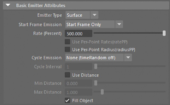
Figure 15.22 Change the emitter’s emissions.

Figure 15.23 The ice cream at its initial frame

Figure 15.24 The ice cream fluid melting
To see a version of the scene up to this point, open the iceCreamCone_v03.ma scene from the chapter15scenes folder at the book’s web page.
Rendering Fluid Containers
Fluid simulations can be rendered using Maya Software or mental ray®, with identical results for the most part. Because fluids have an incandescent value, they can be used as light-emitting objects when rendering with Final Gathering. If you want the fluid to appear in reflections and refractions, you need to turn on the Visible In Reflections and Visible In Refractions options in the Render Stats section of the fluid’s shape node.
This section demonstrates some ways in which the detail and the shading of fluids can be improved when rendered.
Fluids can react to lighting in the scene, and you can apply self-shadowing to increase the realism. As an example of how to light fluids, a scene with simple clouds has been created for you to experiment with:
- Open the
simpleCloud_v01.mascene from thechapter15scenesfolder at the book’s web page. -
Play the animation to frame 100. A simple cloud appears in the center of the scene.
The scene contains a fluid container, an emitter, a plane, and a light. The scene is already set to render using mental ray at production quality.
- Open the Render View window, and render the scene from the perspective camera. A puffy white cloud appears in the render. Store the render in the Render View window (see Figure 15.25, left image).
-
Select the fluid1 node, and open the Attribute Editor to the fluidShape1 tab. Scroll down to the Lighting section at the bottom of the editor.
The Lighting section contains two main settings: Self Shadow and Real Lights. When Real Lights is off, the fluids are lit from a built-in light. Maya has three Light Type options when using an internal light: Directional, Point, and Diagonal. Using an internal light will make rendering faster than using a real light.
When using a Directional internal light type, you can use the three fields labeled Directional Light to aim the light. The Diagonal internal light is the simplest option; it creates lighting that moves diagonally through the x- and y-axes of the fluid. The Point internal light is similar to using an actual point light; it even lets you specify the position of the light and has options for light decay just like a regular point light. These options are No Decay, Linear, Quadratic, and Cubic. For more information on light decay, consult Chapter 7, “Lighting with mental ray.”
You can use the options for Light Color, Brightness, and Ambient Brightness to modify the look of the light. Ambient Diffusion will affect the look of the cloud, regardless of whether you use internal or real lights. Ambient Diffusion controls how the light spreads through the fluid and can add detail to shadowed areas.
- Turn on Self Shadow. You’ll see that the cloud now has dark areas at the bottom in the perspective view. The Shadow Opacity slider controls the darkness of the shadows.
-
Create a test render, and store the render in the Render View window (see Figure 15.25, middle image).
Shadow Diffusion controls the softness of self-shadowing, simulating light scattering. Unfortunately, it can be seen only in the viewport. This effect will not appear when rendering with software (Maya Software or mental ray). The documentation recommends that, if you’d like to use Shadow Diffusion, you render a playblast and then composite the results with the rest of your rendered images using your compositing program.
- In the Outliner, select the directional light and open its Attribute Editor. Under Shadows, select Use Ray Trace Shadows.
- Select fluid1 and, in the Lighting section under the fluidShape1 tab, deselect Self Shadow and select Real Lights.
- In the Render Stats section, make sure that Casts and Receive Shadows are on.
- Create another test render from the perspective camera (see Figure 15.25, right image).
- Save the scene as
simpleCloud_v02.ma.

Figure 15.25 Render the cloud with built-in lights (left image). Enable Self Shadows (center image). Then render the cloud using a directional light that casts raytrace shadows (right image).
When you render using Real Lights, the fluid casts shadows onto other objects as well as itself. When rendering using real shadow-casting lights, make sure that Self Shadow is disabled to avoid calculating the shadows twice. You can see that rendering with Real Lights does take significantly longer than using the built-in lighting and shadowing. Take this into consideration when rendering fluid simulations.
To see a version of the final scene, open the simpleCloud_v02.ma scene from the chapter15scenes folder at the book’s web page.
Creating Fluids and nParticle Interactions
Fluids and nParticles can work together in combination to create a near-limitless number of interesting effects. You can use nParticles as fluid emitters, and you can also use a fluid to affect the movement of nParticles as if it were a field. Next we’ll cover two quick examples that show you how to make the systems work together.
Emitting Fluids from nParticles
In this section, you’ll see how you can emit fluids into a 3D container using nParticles, and you’ll learn about the Auto Resize feature that can help you optimize calculations for fluids.
-
Open the
rockWall_v01.mascene from thechapter15scenesfolder at the book’s web page. Rewind and play the scene.In this scene, nParticles are emitted from a volume emitter. A rock wall has been modeled and turned into a collision object. If you watch the animation from camera1, you’ll see that the scene resembles the wall of a volcanic mountain during an eruption.
- Stop the animation, and switch to the perspective camera.
- In the FX menu set, open Fluids ➣ Create 3D ➣ ❒. Uncheck Add Emitter and choose Apply And Close. The 3D container is added to the scene (see Figure 15.26).
- Set Translate Y of the container to 1.26 and Translate Z to 1.97.
- Open the Attribute Editor for the fluid1 node. Switch to the fluidShape1 tab, and set Base Resolution to 30.
- In the Outliner, select the nParticle1 node and Ctrl/Cmd+click the fluid1 node.
- Choose Fluids ➣ Add/Edit Contents ➣ Emit From Object ➣ ❒.
- In the options, use the following settings:
- Emitter Type: Surface
- Density Rate: 10
- Heat Rate and Fuel Rate: 0
- Click Apply to create the emitter. The new fluid emitter is parented to the nParticle1 node.
- Rewind and play the scene. As the nParticles enter the fluid container, they leave a trail of smoke that rises and gathers at the top of the container (see Figure 15.27).
- Open the Attribute Editor for the fluid1 node. Set Boundary X, Boundary Y, and Boundary Z to None. This will keep the fluid from becoming trapped at the sides of the container.
- Scroll down to the Auto Resize rollout panel. Expand this, and select Auto Resize.
-
Rewind and play the simulation.
Auto Resize causes the fluid container to change its shape automatically to accommodate the fluid (see Figure 15.28). The Max Resolution slider sets a limit to the resolution. When you use Auto Resize, be mindful of the maximum size of the entire simulation; think about what will be within the rendered frame and what will be outside of it. You don’t want to waste resources calculating fluid dynamics that will never be seen in the final render.
The problem with this setup is that as the nParticles fall off the bottom edge of the rockWall collision object, the fluid container stretches downward to accommodate their position. Also, as the fluid rises, the container stretches upward to contain the fluid. There are a couple of strategies that you can use so that the Auto Resize feature does not stretch the container too far. These strategies are discussed in the following steps.
- Open the Attribute Editor for the fluid1 node. In the Contents Details section, expand the Density rollout panel.
-
Set Buoyancy to 0.25 and Dissipation to 1.
These settings will keep the fluid from rising indefinitely, which will limit stretching of the fluid in the upward direction. They also help to keep the smoke trails left by the bouncing nParticles a little more defined.
To keep the fluid1 container from stretching downward forever, you can kill the nParticles as they fall off the bottom edge of the rockWall collision object. One way to do this is to lower the life span; however, this strategy can backfire because some of the nParticles that take longer to bounce down the wall may disappear within the camera view, which can ruin the effect. A better solution is to write an expression that kills the nParticles when they fall below a certain point on the y-axis.
- Select the nParticle1 object in the Outliner, and open its Attribute Editor.
- In the Lifespan rollout panel toward the top, set Lifespan Mode to LifespanPP Only.
- Scroll down to the Per Particle (Array) Attributes section. RMB-click the field next to Lifespan PP, and choose Creation Expression.
-
In the Expression field, type
lifespanPP=8;.This creation expression creates an overall lifespanPP so that each nParticle that is born will have a maximum life span of 8 seconds. This should be enough time so that slower-moving nParticles don’t die before leaving the frame.
- In the Expression Editor, click the Runtime Before Dynamics radio button. Runtime expressions calculate every frame of the simulation and can override the settings established by the creation expression.
-
Type the following into the Expression field:
vector $pPos = position;
float $yPos = $pPos.y;
if($yPos<-4)
{
lifespanPP=0;
}
This expression says that if the Y position of the nParticle is less than –4, then the nParticle’s life span is 0 and the nParticle dies. You need to jump through a few small hoops to get this to work properly. First, you need to access the Y position of the nParticle—which, because of the expression syntax in Maya, cannot be done directly. In other words, you can’t just say
if(position.y<-4). Instead, you have to set up some variables to get to the Y position. That’s just a quirk of the expression syntax. Thus the first line of the expression creates a vector variable called$pPosthat holds the position of the nParticle. The second line creates a float variable called$yPosthat retrieves the Y value of the$pPosvector variable. Now you can use$yPosin theifstatement as a way to access the Y position of each nParticle. In Figure 15.29, you can see the setup of two different expressions applied to the same attribute. The expression on the left is applied at the particle’s creation while the expression on the right is applied at runtime before dynamics. For more information on nParticle expressions, consult Chapter 12. - Click Create to make the expression. If there are no syntax errors, rewind and play the scene. The nParticles should die off as they leave the bottom of the rockWall.
- Save the scene as
rockWall_v02.ma.

Figure 15.26 A 3D fluid container is added to the scene and positioned over the polygon wall.
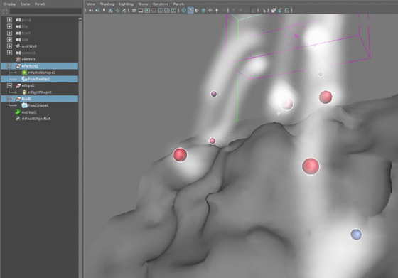
Figure 15.27 The nParticles emit fluids as they enter the container.

Figure 15.28 The fluid container automatically resizes to accommodate the emitted density.

Figure 15.29 Per-particle expressions are created to kill the nParticles when they fall below –4 units on the y-axis.
To see a version of the scene up to this point, open rockWall_v02.ma from the chapter15scenes folder at the book’s web page.
Creating Flaming Trails
To finish the look, you can edit the fluid settings so that the trails left by the nParticles look like flames.
- Continue with the scene from the previous section, or open the
rockWall_v02.mascene from thechapter15scenesfolder at the book’s web page. - Play the scene for about 40 frames.
- Select the fluid1 node, and open its Attribute Editor.
- In the Contents Method section, set Temperature and Fuel to Dynamic Grid.
- Scroll down to the Contents Details section and, in the Temperature section, set Buoyancy to 0.25 and Dissipation to 0.5.
- In the Fuel section, use the following settings:
- Reaction Speed: 0
- Ignition Temperature: –1
- Max Temperature: 1
-
Heat Released: 1
Since Ignition Temperature is at –1, a reaction should occur regardless of how much temperature is released.
-
In the Shading section, set Transparency to a dark gray, and set Glow Intensity to 0.1.
When rendering a sequence using a glow, you should always deselect the Auto Exposure setting in the shaderGlow1 node to eliminate flickering that may occur when the animation is rendered.
- In the Color section under the Shading rollout, click the color swatch and set the color to black.
- The Incandescence ramp should be set to Temperature already. If not, choose Temperature from the menu next to Incandescence Input.
- In the Outliner, expand the nParticle1 node, select the fluidEmitter1 node, and open its Attribute Editor.
- Under Fluid Attributes, use the following settings:
- Heat Method: Add
- Heat/Voxels/Sec: 100
- Fuel Method: Add
- Fuel/Voxels/Sec: 100
-
Rewind and play the animation. You should see flaming trails left behind each nParticle (see Figure 15.30).
You can improve the look by experimenting with the settings, as well as by increasing the Base Resolution and Max Resolution settings in the Auto Resize section.
- Save the scene as
rockWall_v03.ma.

Figure 15.30 The nParticles leave flaming trails as they bounce down the side of the rock wall.
To see a version of the scene up to this point, open the rockWall_v03.ma scene from the chapter15scenes folder at the book’s web page.
Creating Water Effects
Creating believable water or liquid effects in the past required a mixture of particle and fluid simulations. This was a difficult process that fell short on functionality and realism. To solve this problem, Maya 2015 introduced Bifrost, a procedural engine specifically designed for liquid effects. Bifrost’s predecessor was Exotic Matter’s Naiad. Autodesk acquired the Naiad fluid-simulation software in 2012.
Bifrost Liquid Simulation
![]()
The Bifrost engine differs from Maya Fluids and particle simulations by using a FLIP solver. A FLIP solver is a hybrid of sorts, using features from both particle systems and fluid simulations. As a result, water volume and splashing effects are handled with the same solver. The resulting liquid simulation is stable and highly accurate.
There are several components to a Bifrost liquid. Here is an explanation of the nodes and attributes required for a simulation:
Bifrost The bifrost node is the root of the simulation. It controls the display of the liquid in the viewport and is the conduit for all of the other nodes and attributes. The bifrost node is represented by a bounding box based on the overall size of your liquid (see Figure 15.31). As the dimensions of your liquid change, so does the size of the bifrost node.

Figure 15.31 The bifrost node is the box surrounding the sphere.
bifrostLiquid This is the actual container for the liquid. Each container has its own solver settings allowing for independent control over start frame and gravity. The bifrostLiquid node is where you control the resolution or voxel size of the liquid. Figure 15.32 shows the bifrostLiquid icon.

Figure 15.32 The bifrostLiquid node is represented by a single icon of two perpendicular circles and a red locator.
bifrostMesh The bifrostMesh node exists so that the liquid can be converted to polygon geometry. Rendering the liquid as a mesh allows for advanced shading features not available in its particle or voxel form. You can turn the mesh on or off at any point during the simulation from within the bifrost node (see Figure 15.33).

Figure 15.33 The bifrost liquid has a built-in meshing feature to convert the simulation to polygons.
Bifrost Emitter A liquid simulation cannot be created without an emitter. Any polygon geometry can be an emitter. When a mesh is used as an emitter, a new Bifrost rollout is added to its shape node. Figure 15.34 shows the additional attributes.

Figure 15.34 A Bifrost rollout is added to objects being used as emitters.
Liquid simulation with Bifrost requires very little effort since the solver handles all of the intricacies of the liquid’s motion. Furthermore, Bifrost is multithreaded and can take full advantage of your computer’s hardware. The following exercise takes you through the process of creating a Bifrost liquid simulation:
- Open the
pool_v01.mascene from thechapter15scenesfolder at the book’s web page. The scene contains a diving platform, a container, a ball, and a pool. The pool is on a layer with its visibility turned off. The ball is a rigid-body simulation and designed to drop into the pool. - Select the container and choose Bifrost ➣ Liquid. The container is filled with a liquid represented by particle points (see Figure 15.35).
- Turn the visibility off for the CONTAINER layer and turn the visibility on for the POOL layer.
- Make the liquid collide with the pool, ground, and ball. With bifrost1 selected, Shift+click the pool, ground, and ball. Choose Bifrost ➣ Collider under the Add section. The objects now collide with the liquid. The Bifrost liquid may disappear at this point. This happens because the liquid is trying to cache automatically. Press the double back arrows on the timeline controls to go back to the first frame of the playback range. Even though you may already be at the first frame, this forces the Bifrost liquid to update and then be visible again in the viewport.
-
Select bifrostliquid1. Notice the green bar at frame 1 in the timeline. Click Play. Two things happen. First, the animation plays based on the values in the Time slider. A yellow bar fills the timeline as the animation progresses. This bar signifies the uncached frames of the liquid simulation. The second thing is that the liquid begins to cache. The cached frames are represented by a green bar in the timeline that overlaps the yellow bar. If playback is set to Continuous, every loop of the animation will show more and more of the finished simulation. At any point, you can click the Stop button in the lower-right corner of the interface. The progress of the simulation is also displayed here (see Figure 15.36).
Liquid simulations are saved to a scratch cache. This allows you to watch the simulation at a decent frame rate. When you make a change to one of the bifrost nodes, the scratch cache is removed. Playing the simulation will generate a new scratch cache. Making changes to a secondary object, like a collider, does not cause the scratch to be removed. You can manually remove the scratch cache by choosing Bifrost ➣ Flush Scratch Cache.
-
During the simulation, the liquids spill onto the ground object and flow into empty space. Figure 15.37 shows the liquids at frame 210.
Liquid falling into the open air unnecessarily complicates the simulation. To prevent the liquid from traveling too far or off camera, you can introduce a kill plane. Select bifrost1 and choose Bifrost ➣ Killplane from the Add section.
- Scale bifrostKillplane1 uniformly to 22.0 units and translate it to –1.0 in the y-axis. The actual scale of the kill plane is irrelevant. Increasing its scale simply makes it easier to see and select. Click Play to re-create the scratch cache. Figure 15.38 shows the results at frame 210.
- The scale of the pool water looks too large. You can decrease the voxel size in order to increase the resolution of your liquid. Doing so effectively reduces the scale of the liquid. Go to frame 1 and select bifrostLiquid1. In the Channel Box, set Master Voxel Size to 0.20. Depending on the speed of your computer, the lower voxel size may take hours to solve.
- The smaller voxel size makes the liquid more reactive to forces applied against it. In this case, that means the falling ball is going to make a much bigger splash. This may not always be the desired result. To tame the results, you can increase the gravity. Change Gravity Magnitude to 17.6 (see Figure 15.39).
- Instead of using the scratch cache, create a permanent cache file. This will prevent any accidental loss of the cache. Choose Bifrost ➣ Compute And Cache To Disk ➣ ❒.
- Choose a cache directory and give the cache a name. Set the range to be cached and click Create.
- Save the scene as
pool_v02.ma.

Figure 15.35 Create a liquid from the container geometry.

Figure 15.36 The liquid simulation is cached during playback.

Figure 15.37 The liquid falls over the edge of the ground object.

Figure 15.38 The kill plane prevents the liquids from falling.

Figure 15.39 Changing the gravity magnitude helps to reduce the effects of forces on the liquid.
To see a version of the scene up to this point, open the pool_v02.ma scene from the chapter15scenes folder.
Shading Bifrost Liquids
![]()
You can render the liquid simulation in two ways. Voxel rendering is the default method. This is similar to how Maya Fluids render. As with Maya Fluids, you can also convert the simulation data into a polygon mesh. Mesh nodes are created along with the liquid; therefore, a separate conversion is not necessary. You can enable the mesh for a liquid at any point.
The Bifrost liquid is automatically assigned a shader. Enabling the mesh option for the liquid allows you to take full advantage of the shader’s features and different rendering techniques. The following example takes you through the steps to render a realistic-looking liquid:
- Continue with the scene from the previous section, or open the
pool_v02.mascene from thechapter15scenesfolder at the book’s web page. -
Select liquid1 from under the bifrostLiquid1 hierarchy. In the Channel Box, set Meshing Enable to On. A polygon mesh is created, matching the particle volume.
With the mesh turned on, your simulation will run slower. However, the liquid is already cached. This means that you can skip frames to see the results of the mesh.
- Go to frame 90. The mesh will update accordingly. The ball, however, will not update since it is an uncached bullet simulation (see Figure 15.40).
- Create a layer named BIFROST. Add bifrostliquid1 and turn off the visibility for the layer.
- Select liquidShape1. Change Meshing Surface Radius to 1.0. The smaller surface radius reduces the volume of the polygon mesh, in this case giving the water finer details. Compare Figure 15.41 with Figure 15.40.
- Open the Hypershade and choose bifrostLiquidMaterial1. Open its Attribute Editor.
-
Most of the default values of the liquid material are already set for a convincing water look. Look at the Reflection rollout. Reflection Color is pure white and Reflection Weight is set to 1.0. These are good settings; however, the scene does not have an environment to reflect.
Select the Perspective camera and open its Attribute Editor. Choose the perspShape tab and expand the Environment rollout. Change Background Color to a sky blue. Render a test frame to see the water reflect the blue sky (see Figure 15.42).
- Under the Refraction/Transmission rollout for the bifrostLiquidMaterial, change the Color value. Using the HSV color scale, set Value to 0.85. Next, change the Transparency, located under the grayed Refraction Color Remap rollout, to 1.0 (see Figure 15.43).
- Select Use Color At Max Distance and set the Max Distance value to 10.0. Using a maximum distance for the refraction causes the water to fade to black at the distance value.
- With the maximum distance enabled, you can change the color of the refraction based on light passing through the water’s thickness. Adding a color for the water to fade to gives the liquid more visual depth. Use the following parameters to set the color value:
- Hue: 200.0
- Saturation: 0.298
- Value: 0.146
- When water gets agitated, it bubbles and reflects more light. We identify this as foam. Currently, the foam effect is too extreme, and the water turns white. Expand the Surface Foam rollout. Set Color Remap Channel to Velocity. Set Foam Weight to 0.5. Figure 15.44 shows the water with its new foam attributes.
- Save the scene as
pool_v03.ma.

Figure 15.40 Create a polygon mesh by enabling meshing on the bifrost node.

Figure 15.41 Decrease the surface radius to 1.0.

Figure 15.42 The water mesh reflects its environment.

Figure 15.43 Add transparency to the water.

Figure 15.44 Adding foam completes the look of the water.
To see a version of the scene, open the pool_v03.ma scene from the chapter15scenes folder at the book’s web page. You can also watch the rendered version of the simulation from the chapter15movies folder.
Guiding Liquid
![]()
You can control the shape of a liquid simulation by using guide geometry. The guide geometry can be static, animated, or even deformed. To optimize your scene, you can even use Alembic cached geometry. When a Bifrost liquid is being driven by guide geometry, only the liquid at the top of the guide is simulated. You can control the depth at which the liquid is simulated through a minimum simulation depth. Through guides, you can shape your liquid into virtually anything. The following example takes you through the steps of converting a motion-captured driven character into a liquid entity:
- Start with a new Maya scene. Open the Visor and click the Mocap Examples tab. MMB-drag
fight3.mainto the Maya viewport. - The motion capture is imported into the scene with real-world units and is extremely large. Press a to frame the scene elements.
- Select the character geometry and choose Bifrost ➣ Liquid. The Bifrost liquid may not update on the model immediately. To force it, play through the timeline for a few frames and then return it to frame 1. The liquid container’s bounding box should envelop the character (see Figure 15.45).
- Currently, the mesh will emit the liquid as it moves. However, the liquid will not move with the character to retain the character’s shape. Shift-select fight3_skin and bifrost1. Choose Bifrost ➣ Guide from the Add section. Adding the guide may take a few minutes to update.
- The guide is not automatically turned on. Select the bifrostliquidContainer1 node in the Attribute Editor. Expand the Guided Simulation rollout and choose Enable.
- You can now play through the timeline and see the Bifrost liquid following the character’s motions. Figure 15.46 shows the results from frame 20.
- The liquid adheres to the original form of the character better, but liquid is still spraying too much to identify the character underneath. For an added effect, increase the viscosity of the liquid. Under the bifrostliquidContainer1 tab in the Attribute Editor, expand the Viscosity rollout. Set Viscosity Scale to 0.8. Figure 15.47 shows the final results at frame 20.

Figure 15.45 Add a Bifrost liquid to the character’s mesh.

Figure 15.46 The geometry guides the liquid at frame 20.

Figure 15.47 Adding viscosity keeps the water from spraying too much.
Creating an Ocean
The ocean fluid effect uses a surface and a special Ocean shader to create a realistic ocean surface that can behave dynamically. The Ocean shader uses an animated displacement map to create the water surface. Ocean surfaces can take a while to render, so you should consider this when planning your scene.
You can find all of the controls needed to create the ocean on the oceanShader node. This node is created and applied automatically when you create an ocean. In this example, you’ll create the effect of a space capsule floating on the surface of the ocean:
- Open the
capsule_v01.mascene from thechapter15scenesfolder at the book’s web page. This scene has the simple space capsule model used in Chapter 12. - Switch to the FX menu, and choose Fluids ➣ Ocean.
- Rewind and play the scene. You’ll see the preview plane move up and down. This demonstrates the default behavior of the ocean (see Figure 15.48).
-
In the Outliner, select the transform1 node and open the Attribute Editor. Switch to the oceanShader1 tab.
You’ll find all of the controls you need to change the way the ocean looks and behaves in the Ocean shader controls. Each control is described in the Maya documentation, but many of the controls are self-explanatory.
- Expand the Ocean Attributes rollout panel. To slow down the ocean, set Wave Speed to 0.8. You can use Observer Speed to simulate the effect of the ocean moving past the camera without the need to animate the ocean or the camera. Leave this setting at 0.
-
To make the ocean waves seem larger, increase Wave Length Max to 6. The wavelength units are measured in meters.
To make the ocean seem a little rougher, you can adjust the Wave Height edit curve. The Wave Height edit curve changes the wave height relative to the wavelength. If you edit the curve so that it slopes up to the right, the waves with longer wavelengths will be proportionally taller than the waves with shorter wavelengths. A value of 1 means that the wave is half as tall as it is long. When you edit this curve, you can see the results in the preview plane.
Wave Turbulence works the same way, so by making the curve slope up to the right, longer waves will have a higher turbulence frequency.
Wave Peaking creates crests on top of areas that have more turbulence. Turbulence must be a nonzero value for wave peaking to have an effect.
- Experiment with different settings for the Wave Height, Wave Turbulence, and Wave Peaking edit curves (see Figure 15.49). Create a test render from the perspective camera to see how these changes affect the look of the ocean.
- To make the capsule float in the water, select the capsule and choose Fluids ➣ Create Boat ➣ Float Selected Object(s).
- In the Outliner, select Locator1 and open its Attribute Editor.
- In the Extra Attributes section, set Buoyancy to 0.01 and Start Y to –3.
- Select the capsule, and rotate it a little so that it does not bob straight up and down.
- Select the transform1 node, and open the Attribute Editor to the oceanShader1 tab.
- In the Common Material Attributes section, set Transparency to a dark gray color. This allows you to see some of the submerged parts of the capsule through the water. The oceanShader already has a refraction index of 1.3, so the water will refract light.
- Set Foam Emission to 0.355. This shades the peaks of the ocean with a light color, suggesting whitecaps.
- Create a test render of the scene from the perspective camera (see Figure 15.50).
- Save the scene as
capsule_v02.ma.

Figure 15.48 The ocean effect uses a preview plane to indicate the behavior of the ocean.
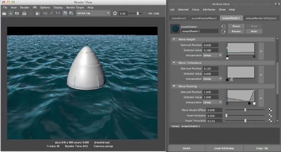
Figure 15.49 You can shape the ocean by editing the Wave Height, Wave Turbulence, and Wave Peaking edit curves.

Figure 15.50 Render the capsule floating in the water.
To see a finished version of the scene, open the capsule_v02.ma scene from the chapter15scenes folder at the book’s web page.
This is a good start to creating a realistic ocean. Take a look at some of the ocean examples in the Visor to see more advanced effects.
The Bottom Line
Use fluid containers. Fluid containers are used to create self-contained fluid effects. Fluid simulations use a special type of particle that is generated in the small subunits (called voxels) of a fluid container. Fluid containers can be 2D or 3D. Two-dimensional containers take less time to calculate and can be used in many cases to generate realistic fluid effects.
Master It Create a logo animation that dissolves like ink in water.
Create a reaction. A reaction can be simulated in a 3D container by combining temperature with fuel. Surfaces can be used as emitters within a fluid container.
Master It Create a chain reaction of explosions using the Paint Fluids Tool.
Render fluid containers. Fluid containers can be rendered using Maya Software or mental ray. The fluids can react to lighting, cast shadows, and self-shadow.
Master It Render the
TurbulentFlame.maexample in the Visor so that it emits light onto nearby surfaces.
Use fluids with nParticles. Fluid simulations can interact with nParticles to create a large array of interesting effects.
Master It nCloth objects use nParticles and springs to simulate the behavior of cloth. If fluids can affect nParticles, it stands to reason that they can also affect nCloth objects. Test this by creating a simulation where a fluid emitter pushes around an nCloth object.
Create water effects. Ocean effects are created and edited using the Ocean shader. Objects can float in the ocean using locators.
Master It Create an ocean effect that resembles stormy seas. Add the capsule geometry as a floating object.