Chapter 5

Point Estimation

5.1. Generalities

5.1.1. Definition – examples

Let be a statistical model and let g be a map from Θ to a set A with a σ-algebra .

DEFINITION 5.1.– An estimator of g(θ) is a measurable map from E to A.

In an estimation problem, the set of decisions is therefore the set where the function g of the parameter takes its values. It acts to, in light of the observations, admit a value for g(θ) (a “function of the parameter”).

COMMENT 5.1.– If the model is written in the form , we may consider g to be a function of P.

EXAMPLE 5.1.– In all of the examples below, .

1) .

2) .

3) , where uθ denotes a uniform distribution on [0, θ], ; g(θ) = θ.

4) P = a set of distributions of the form , where Pm, D is a probability on with expectation value m and covariance matrix D; g(θ) = (m, D).

5) P = the set of distributions of the form P⊗n, where P is a probability on with a density fP with respect to the Lebesgue measure λ (or a known, or a square-integrable density, etc.); g(θ) = θ = fP.

Here , or L2(λ), etc., respectively).

6) P = the set of distributions of the form P⊗n, where P describes the set of all probabilities on ; g(θ) = θ = FP (distribution function of P) (or also g(θ) = P).

7) P = the set of distributions of the form P⊗n, where P describes the set of distributions on with positive density such that, if (X, Y) follows such a distribution, x E(Y|X = x) is defined (Y is therefore integrable or positive); g(θ) = g(P) = E(Y | X = x).

8) P = the set of distributions of the form P⊗n, where P describes the set of probabilities on with compact support in SP; g(θ) = g(P) = SP.

COMMENT 5.2.– We see that A may take a great variety of forms: , a function space and even a class of sets (point 8) which may also, after taking the quotient, be equipped with a metric (d(A, B) = λ(A Δ B)).

5.1.2. Choice of a preference relation

1) In general, if , we define a preference relation using the loss function:

The associated risk function is then the quadratic error or the quadratic risk:

where T denotes the estimator (i.e. the decision function).

If Eθ(T) = g(θ) and R(θ, T) is the variance of T, we write .

COMMENT 5.3.– We may also use loss functions of the form c(θ)(g(θ) − a)2, which leads to the same preference relation between estimators, provided that c(θ) is strictly positive for all θ.

The loss function |g(θ) − a|, which generally provides a different preference relation, is sometimes used. However, it gives a less convenient cost function than the quadratic error.

2) If , we define a preference relation in a similar way.

First of all, given X = (X1, …, Xp), a random variable with values in such that , we define its matrix of second-order moments by setting:

For centered X, CX coincides with the covariance matrix of X.

We may consider CX as defining a symmetric linear operator of . It is then straightforward to verify that:

[5.1]

where denotes the scalar product of .

In particular,

[5.2]

Conversely, if D is a symmetric linear operator of having property [5.2], it also has property [5.1], since

From this, we deduce that D = CX.

We now define a partial order relation on the symmetric linear operators of by posing if and only if for all .

PROPERTIES.–

The above property allows us to define a preference relation on the set of estimators of g(θ) by writing:

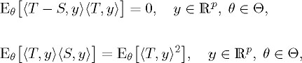
[5.3]

If S and T are of square-integrable norm (for all θ), we also have:

Relation may be interpreted in the following way: if and only if, for all is preferable to 〈S, y〉 as an estimator of 〈g(θ),y〉 with respect to the quadratic error.

3) Relation has the inconvenience of not allowing a numerical measure of the risk associated with an estimator. This observation leads us to define a relation by the equivalence

[5.4]

This relation is less refined than the previous one since, if T S and if {e1, …, ep} denotes the canonical basis of , then we have, for all θ ∈ Θ,

Note that if T is of square-integrable norm, then is the trace of the matrix CT−g(θ).

5.2. Sufficiency and completeness

5.2.1. Sufficiency

In estimation theory, the Rao–Blackwell theorem takes the following form:

THEOREM 5.1.– Let g be a function of the parameter, with values in , and let T be an estimator of g(θ) that is integrable for all θ. If U is a sufficient statistic and if denotes the σ-algebra generated by U, then we have:

PROOF.– The Rao–Blackwell theorem states that is preferable to 〈T, y〉 for the estimation of 〈g(θ, y). Since , we deduce that and consequently .

APPLICATION: Symmetrization of an estimator.– Given a statistical model of the form where P0 is a family of probabilities on , let us consider the statistic S defined by:

where x(1) denotes the smallest xi, x(2) denotes the smallest remaining xi, …, and x(n) denotes the largest xi.

This statistic is called the order statistic. The σ-algebra that generates it is the σ-algebra of symmetric Borel sets (i.e. the σ-algebra of Borel sets that are invariant under permutation of the coordinates). The -measurable random variables are the symmetric random variables.

We then have the following theorem.

THEOREM 5.2.– If the statistical model is of the form , then the order statistic is regularly sufficient.

PROOF.– Let and , then

and, since B is symmetric, we have the equality:

where S denotes the set of permutations of the first n natural numbers.

The function being -measurable, it constitutes a regular version of ; this version is independent of P.

If T is an integrable estimator of g(P) with values in , then Theorems 5.1 and 5.2 show that is preferable to T, as is the symmetrization of T, i.e.

since the distribution determined by U(x1, …, xn) is .

CONCLUSION.– If the observations come from a sample, we may restrict ourselves to the study of estimators that are symmetric with respect to the data.

5.2.2. Complete statistics

DEFINITION 5.2.– Let be a statistical model and let be a sub-σ-algebra of is said to be complete if for every real, -measurable statistic U:

A statistic S is said to be complete if the sub-σ-algebra that generates it is complete.

Placing ourselves under the hypotheses of Theorem 5.1, and denoting by the set of estimators T′ of g(P) such that EP(T′) = EP(T) for all P ∈ P, we then have:

THEOREM 5.3. Lehmann–Scheffé theorem.– If U is a regularly sufficient and complete statistic, is optimal in for and .

PROOF.– We first note that (a property of the conditional expectation). However,

with

Since U is complete, we deduce that P [φ(U) = 0] = 1, ∀P ∈ P. is therefore unique, up to an equivalence, and it is preferable to T for all : it is optimal in .

EXAMPLE 5.2.–

1) Given the exponential model (Example 4.3, section 4.3) of density A(θ) · exp with respect to the Lebesgue measure λp on , where θ ∈ Θ is an open convex set in , T is sufficient and complete. Indeed,

The injectivity of the Laplace transform1 then implies that the measure with sign φ·λT−1 is zero, which means that φ = 0 λT−1 almost everywhere, i.e. φ(T) = 0 λ almost everywhere, from which Pθ [φ(T) = 0] =1.

2) The order statistic U is sufficient and complete in P, and in where denotes the set of discrete distributions of as well as in , where denotes the set of distributions of which have a density of the form with the and where the Ij are pairwise-disjoint bounded intervals.

Let us show this result for (and therefore for P as well); for , we may consult [FRA 57, pp. 27–30], but the proof is similar – it also uses the following lemma:

LEMMA 5.1.– Let (p1, …, pn) be a homogeneous polynomial such that (p1, …, pn) = 0 for (p1, …, pn) ∈ [0, 1]n and ∑ pi = 1. Q is then identically zero.

PROOF.– Q being homogeneous, we may replace the conditions on the pi with the conditions p1 ≥ 0, …, pn ≥ 0.

If we then write as a polynomial in pn, then the condition (p1, …, pn) = 0 for p1 ≥0, …, pn ≥ 0 leads to the fact that the coefficients of pn are zero. Since the coefficients are homogeneous polynomials with n − 1 variables, we deduce the lemma by induction.

It now suffices to consider , and to write that for a symmetric function g:

and deduce that , as the integral is a homogeneous nth degree polynomial that vanishes identically (Lemma 5.1) and the coefficient of p1 … pn is , since g is symmetric.

5.3. The maximum-likelihood method

5.3.1. Definition

Point estimation methods vary considerably, and depend greatly on the problem under consideration. We first refer to the Bayesian methods which we developed in section 2.3. One quite general method is that of the maximum likelihood.

DEFINITION 5.3.– Let , be a dominated statistical model, and let T be an estimator of Θ. We say that T is a maximum-likelihood estimator if:

REMARK 5.1.–

1) If Θ is an open set of and if f(x, ·) is differentiable for all x, then a maximum-likelihood estimator is a solution to the system of likelihood equations:

[5.5]

Of course, a solution to [5.5] is not necessarily a maximum-likelihood estimator.

2) The random function f(X, ·) is called the likelihood associated with the considered model.

EXAMPLE 5.3.–

1) X = (X1, …, Xn) a sample of . We set

The likelihood equation:

has the solution

We easily verify that

(using the fact that, for u > 0, u – 1 – log u ≥ 0).

2) X = (X1, …, Xn) a sample with uniform distribution on . Then:

X(1) and X(n) – 1 are both maximum-likelihood estimators for θ: the maximum-likelihood estimator is not unique.

3) Θ = the set of compact convex sets of with positive Lebesgue measure.

Pθ = a uniform distribution on θ, θ ∈ Θ.

X = (X1, …, Xn) a sample taken from Pθ, n ≥ 3.

A maximum-likelihood estimator of θ is the convex envelope of (X1, …, Xn). Indeed,

A maximum-likelihood estimator is sought among the θ such that f(X, θ) > 0, therefore among the θ that contain the convex envelope of the sample. Among these, it is necessary to seek those which maximize f(X, θ) and therefore minimize λ(θ): the result is the convex envelope.

5.3.2. Maximum likelihood and sufficiency

PROPOSITION 5.1.– If Y is a sufficient statistic for θ, every maximum-likelihood estimator is, up to an equivalence, a function of T.

PROOF.–

– f(x, θ) = g[T(x), θ] h(x) (factorization theorem).

– The set of x such that h(x) = 0 is of zero measure for all Pθ.

Now, if h(x) > 0, a maximum of f(x, θ) is also a maximum of g [T(x), θ] and therefore a function of T(x).

COMMENT 5.4.– A maximum-likelihood estimator is not always a sufficient statistic.

EXAMPLE 5.4.– X = (X1, …, Xn) a sample of a uniform distribution on [θ, 2θ], 0 < θ < +∞. (X(1), …, X(n)) is sufficient and minimal, and the maximum-likelihood estimator of X(n)/2 is not therefore sufficient.

5.3.3. Calculating maximum-likelihood estimators

It is often difficult to explicitly solve the likelihood equation, even in the regular cases where the solution is unique.

We first indicate an important case where the maximum-likelihood estimator is unique:

PROPOSITION 5.2.– If X = (X1, …, Xn) is a sample of size n with density:

θ = (θ1, …, θk) ∈ Θ is an open set in (exponential model), and if the matrix [∂2/(∂θi∂θj)ϕ] is positive-definite, ∀θ ∈ Θ; then the maximum-likelihood estimator of θ is the unique solution to:

[5.6]

COMMENT 5.5.– We will later prove that ϕ is infinitely differentiable.

PROOF.– maximizes . Differentiating, we deduce that is the solution to [5.6] since the fact that [∂2/(∂θi∂θj)ϕ] is positive-definite implies the existence of a unique solution for [5.6] which, furthermore, is a maximum for the density of X.

Let us now give an example where we do not have an explicit solution: if X1, …, Xn is a sample of a Cauchy distribution with density 1/π[1 + (x − θ)2], , then the likelihood equation is written and it may have multiple solutions. We may then use numerical methods:

5.3.3.1. The Newton–Raphson method

We write:

with θ1 given.

For ν = 0, we find, as an approximation of :

In general, we write:

Under regularity conditions, and for large enough k, θk is a good approximation of .

REMARK 5.2.–

1) In the case of the Cauchy distribution (Example 5.4), it is often interesting to take the empirical median as an estimator of θ:

The determination of this estimator does not require any calculation, but is slightly worse than .

2) We will see later that the maximum-likelihood estimator often has good asymptotic properties.

5.4. Optimal unbiased estimators

As we saw in Chapter 2, it is necessary to restrict the set of decision rules in the hope of obtaining an optimal rule for the envisaged problem.

In estimation theory, we are often limited to the search of unbiased, minimum-dispersion estimators.

We will begin by studying some existence conditions of unbiased estimators in a more detailed manner than is generally done: we will see that the existence conditions of such an estimator are quite restrictive.

5.4.1. Unbiased estimation

DEFINITION 5.4.– Let be a statistical model and let g be a map from Θ to . An estimator T of g(θ) is said to be unbiased if for all θ ∈ Θ, T is Pθ-integrable and

EXAMPLE 5.5.–

1) In the case of a sample on is an unbiased estimator of the mean, if it exists.

2) In the case of a sample on and for g(θ) = Fθ(t), where Fθ is the distribution function of Pθ: the empirical distribution function:

is an unbiased estimator of Fθ(t).

In the usual cases, the definition of an unbiased estimator is in agreement with the general definition of an unbiased decision function given in Chapter 2. More precisely, we have the following result:

PROPOSITION 5.3.– Let T be an estimator of g(θ) such that:

1) ,

2) ;

then T is unbiased if and only if:

3) .

PROOF.– For all (θ, θ′) ∈ Θ2, we may write:

Writing the previous relation for θ′ = θ and taking the difference, we obtain:

Moving to expected values, we obtain:

Result (3) is therefore equivalent to:

4) .

Then, if T is unbiased, we have (4) and therefore (3). Conversely, if (3) is satisfied, then we have (4) and taking θ′ such that g(θ′) = Eθ(T) in (4), we deduce that T is unbiased.

5.4.1.1. Existence of an unbiased estimator

Here is a general result relating to the existence of an unbiased estimator obtained by Bickel and Lehmann [BIC 69].

We first give some definitions:

DEFINITION 5.5.– Given a statistic model of the form , an estimator of g(P) is said to be an estimator of order n.

Assuming that g takes values from , we say that g is estimable without bias if there exist a natural number n and an unbiased estimator of order n for g(P).

If g is estimable without bias, the degree of g is the smallest natural number n such that g(P) has an unbiased estimator of order n.

EXAMPLE 5.6.– In , the variance is estimable without bias, with degree 2.

THEOREM 5.4. Bickel–Lehmann theorem.– If P0 is convex, and if g is estimable without bias, then the following conditions are equivalent:

1) the degree of g = n.

2) – g[αP + (1 – α)Q] is a polynomial in α of degree ≤ n, for all (P, Q) ∈ P0 × P0.

– ∀P ∈ P0, ∃Q ∈ P0 such that g [αP + (1 − α)Q] is exactly of degree n.

The conditions of this theorem may seem surprising, but they are clarified by the following remark: if Tn is an unbiased estimator of order n for g, we have:

and the first term in this equality is a polynomial in α of degree ≤ n.

For the proof, we refer to [BOS 87b].

The Bickel–Lehmann theorem shows above all the rarity of parameters allowing an unbiased estimator. It is clear, for example, that the standard deviation is not estimable without bias.

COMMENT 5.6.– We may show that condition (2) of Theorem 5.4 does not assure the existence of an unbiased estimator of g (even if n = 1).

5.4.2. Unbiased minimum-dispersion estimator

THEOREM 5.5.– Let T be an estimator of g(θ) where g takes values in . We suppose that T is unbiased and is such that for all θ. The two following conditions are then equivalent:

1) T is unbiased and of minimum dispersion (i.e. T is optimal for in the family of unbiased estimators with square-integrable norm).

2) For every real-valued statistic U, which is centered and square integrable for all θ, we have:

PROOF.–

−1) 2)

The result being evident for y = 0, we may suppose that y ≠ 0. Then T + αU y is an unbiased estimator for g(θ), of square-integrable norm . Since T is optimal, we have:

from which

Letting α tend to 0+, we note that E_θ [U 〈T , y〉] ≥ 0. We therefore have E_θ [U 〈T , y〉] = 0, otherwise we may make γ < 0 for a well-chosen α < 0.

– 2) 1)

Let S be unbiased such that ; we set . Uy satisfies the hypotheses of (2), therefore

from which

that is

COMMENT 5.7.– Let us set T = (T1, …, Tp). It is clear that in condition (2), we may replace:

with

5.4.2.1. Application to an exponential model

Let P_θ = exp [〈θ, T〉 − ϕ(θ)] · μ, θ ∈ Θ, be an exponential model. We suppose that Θ is an open set in and that μ is a σ-finite measure on .

Let us first of all state the following lemma.

LEMMA 5.2.– ϕ is infinitely differentiable.

PROOF.– To simplify the notation, we will only conduct the proof for p = 1.

Let there be θ0 ∈ Θ and ε > 0 such that [θ0 − 2ε, θ0 + 2ε] ⊂ Θ.

For integer k ≥ 1, we are given a constant ck such that:

Then, for θ ∈]θ0 − ε, θ0 + ε[,

[5.7]

This last function is μ-integrable since:

[5.8]

Inequality [5.7] and the dominated convergence theorem show that we may derive [5.8] k times under the integral sign.

We then have the following theorem:

THEOREM 5.6.– T is an optimal unbiased estimator for grad ϕ(θ) and its covariance matrix is (∂2ϕ/∂θi∂θj).

PROOF.–

1) From Lemma 5.2, we may derive the equality:

from which, setting T(x) = (T1(x), …, Tk(x)),

[5.9]

and

[5.10]

2) Let U be such that EθU = 0, for all θ, i.e.

In , we have (the proof is analogous in ):

and the dominant function is fixed and μ-integrable. We may therefore differentiate under the integral sign:

The second integral vanishes, and finally Eθ(TU) = 0; T is optimal.

5.4.2.2. Application to the Gaussian model

PROPOSITION 5.4.– Let (X1, …, Xn) be a sample of size n (≥ 2) of . Then is unbiased and of minimum dispersion for (m, σ2).

PROOF.– We use Theorem 5.5.

Let U be such that Eθ(U) = 0, then:

[5.11]

We then differentiate with respect to m:

Taking [5.11] into account, we have:

[5.12]

that is

We differentiate again:

[5.13]

Taking account of [5.11] and [5.12], this implies:

We now differentiate [5.11] with respect to σ2:

that is

Yet , therefore

REMARK 5.3.–

1) We have proved both of the following additional results: is optimal and unbiased for m, and (n/n – 1)S2 is optimal and unbiased for σ2.

2) Theorem 5.5 does not directly apply to θ = (m,σ2) (see equation [4.1] in section 4.3).

5.4.2.3. Use of the Lehmann–Scheffé theorem

If T is unbiased and S is a complete and sufficient statistic, Theorem 5.3 affirms that is unbiased and of minimum dispersion.

EXAMPLE 5.7.– For the model where P0 contains the discrete distributions, is optimal and unbiased for the distribution function at the point x, since this estimator is symmetric and the order statistic is then sufficient and complete.

5.4.3. Criticism of unbiased estimators

– Unbiased estimators have, in general, the inconvenience of not being admissible.

EXAMPLE 5.8.–

   1)Let(X1, …, Xn) be a sample of is then preferable to .

   2) In the model is preferable to .

– Some unbiased estimators are not strict (an estimator T of g(θ) is said to be strict if Pθ(T ∈ g(Θ)) = 1, ∀θ ∈ Θ).

EXAMPLE 5.9.– Given the model [θδ(1) + (1 − θ)δ(−1)]⊗n, θ ∈]1/2, 1[, is the best unbiased estimator of 2θ − 1, but it is not strict. sup is strict and preferable to .

5.5. Efficiency of an estimator

5.5.1. The Fréchet-Darmois-Cramer-Rao inequality

We consider the model where Θ is an open set in and we seek to estimate g(θ) where is differentiable. We suppose that dPθ = Lθ · dμ (with Lθ > 0 on a fixed open set in ) and we denote an unbiased estimator of g by T. Then

Supposing that it is possible to differentiate under the integral sign, we obtain:

and

from which

that is

From Schwarz’s inequality, we have:

from which, finally

[5.14]

supposing that I(θ) ≠ 0 and finite for all θ. I(θ) is called the Fisher information. We also say that [5.14] is the information inequality.

5.5.1.1. Calculating I(θ)

1) Since

we have:

that is

[5.15]

2) If we can differentiate a second time under the integral sign, we have:

[5.16]

Indeed, from

we take, by differentiating

hence the result, since

3) Case of independent variables with the same distribution:

Since log , then

and

[5.17]

since Eθ[(∂/∂θ)log f(Xi, θ)·(∂/∂θ) log f(Xj, θ)] is zero for i ≠ j, as the covariance of two independent random variables.

Under the conditions of (2), we also have:

5.5.1.2. Properties of the Fisher information

PROPERTY (α).– Let , i = 1, …, k, be statistical models conforming to the hypotheses of regularity seen previously. We consider the model product . Then, in clear notation,

(whose proof is analogous to that of equation [5.17]).

PROPERTY (β).–

THEOREM 5.7.– Let S be a statistic with values in such that the induced model is dominatedby λm and such that:

[5.18]

where Λ(s, θ) denotes the density of (PθS−1). Then:

[5.19]

and the equality holds if S is sufficient.

PROOF.– Indeed,

Now, if S is sufficient,

from which

and from [5.19],

We deduce that Iθ, S = Iθ.

COMMENT 5.8.– Condition [5.18] is satisfied in the usual cases, as

may be written as:

If we can differentiate under the integral sign, we have:

that is

therefore [5.18] is satisfied.

CONCLUSION.– (α) and (β) are natural properties that we may expect from a quantity of information: I(θ) verifies them under quite general regularity conditions.

5.5.1.3. The case of a biased estimator

Let T be an integrable estimator of g(θ). We set:

T is then an unbiased estimator of g(θ) + B(θ). If B is differentiable and if the regularity conditions of the Cramer–Rao inequality are satisfied, then:

5.5.2. Efficiency

DEFINITION 5.6.– An unbiased estimator T is said to be efficient if:

[5.20]

Existence condition: [5.20] holds if and only if:

therefore if and only if

Integrating, we find:

i.e. the model is exponential.

COMMENT 5.9.– In the particular case where A(θ) = θ, we saw that T is the best unbiased estimator of g(θ) = ϕ′(θ) (Theorem 5.5). The property obtained here is more precise: an unbiased estimator may be optimal without being efficient, as we will see later.

5.5.3. Extension to

THEOREM 5.8.– Let be a statistical model where Θ is an open set in . Let g be a differentiable map from Θ into . We make the following assumptions:

1) Pθ = L(·, θ) · μ where L(x, θ) > 0 μ almost everywhere.

2) Lθ is differentiable and

3) , and the covariance matrix of Iθ of Uθ = grad log L(X, θ) (called a Fisher information matrix) is invertible.

4) T is an unbiased estimator of g(θ) such that the equality:

is differentiable under the integral sign.

Then, if Dθ (T) is the covariance matrix of T,

2 (Cramer –Rao inequality)

where Δθ = ((∂/∂θj) gi (θ)).

PROOF.– Let us set

then, for ,

But

and

and yet, EθUθ = 0, therefore and

So

Bringing together the obtained results, we find:

COROLLARY 5.1.– Under the previous hypotheses and with g(θ) = θ, we find:

PROOF.– In effect, the Cramer–Rao inequality implies here that:

, 3

from which we find the result by using an orthonormal basis of .

5.5.3.1. Properties of the information matrix

We have properties analogous to the case of under regularity hypotheses. The details are left to the reader. We therefore have:

1)

2) Iθ = I1 (θ) + … + Ih(θ) (matrix sum);

3) Iθ,S ≤ Iθ (i.e. Iθ−Iθ,S positive-definite) and the equality holds for sufficient S.

5.5.3.2. Efficiency

The efficiency is defined as in : an estimator is efficient if:

As in , we have:

PROPOSITION 5.5.–Under the hypotheses of the previous theorem, and the additional hypothesis k = p and Δθ is invertible, a necessary condition for the existence of an unbiased estimator is that the family (Pθ) be exponential.

PROOF.– Let T be an efficient unbiased estimator. Then Dθ(Z) = 0, therefore Z = 0 Pθ almost everywhere, therefore also μ almost everywhere. Consequently,

that is

from which, by integrating, we find the result.

The reciprocal: If P_θ = exp [〈θ, T (x)〉 − ϕ(θ)] · μ, θ ∈ Θ is an open set of , then T is an efficient unbiased estimator of grad ϕ(θ).

PROOF.– Theorem 5.5 implies that T is unbiased and that:

but

therefore

Furthermore, from log L(X, θ) = 〈θ, T〉 − ϕ(θ), we take:

from which

then

and finally

COMMENT 5.10.– is optimal but not efficient for the estimation of (m, σ2) in the Gaussian case.

Indeed,

while

In particular, is not efficient for the estimation of σ2. The details of the calculation are left to the reader.

5.5.4. The non-regular case

5.5.4.1. “Superefficient” estimators

In the case of the estimation of a real parameter from a sample, the Cramer–Rao inequality shows that the variance of an unbiased estimator is better by an order of 1/n for n tending to infinity. However, we may sometimes obtain variances of a superior order when the validity conditions of the Cramer–Rao inequality are not met. An estimator with this property is said to be “superefficient”.

EXAMPLE 5.10.– Let X1, …, Xn be a sample of a uniform distribution on [0, θ] is a superefficient unbiased estimator of θ. Indeed, VarθT = θ2/n(n + 2).

5.5.4.2. Cramer–Rao-type inequalities

The differentiability hypotheses of Theorem 5.8 often being inconvenient in practice, numerous authors have demonstrated Cramer–Rao-type inequalities which do not include these conditions. Their results are often in the following form:

PROPOSITION 5.6.– being a statistical model and g being a real-valued function of the parameter, we denote by Uθ,θ′ a real random variable, indexed by G ⊂ Θ × Θ and such that:

(C3) If S and T are two square-integrable estimators of g(θ) such that m(θ) = Eθ(S) = Eθ(T), θ ∈ Θ, then Eθ [Uθ,θ ′ ·T] = Eθ [Uθ,θ′ · S], (θ,θ′) ∈ G. In other words, Covθ [Uθ,θ′ · T] = φm(θ,θ′).

Under these conditions,

where Gθ = {θ′: (θ, θ′) ∈G}.

PROOF.– Schwarz’s inequality is written as:

which allows us to conclude the proof in a straightforward way, taking account of the hypotheses made on Uθ, θ′.

EXAMPLE 5.11.– If Pθ = fθ · λ, we may take Uθ, θ′ = (fθ′/fθ) − 1 on the condition that we suppose θ Pθ to be injective, and that Eθ[(fθ′/fθ)2] < +∞ for (θ, θ′) ∈ G.

We thus obtain the Chapman–Robbins inequality [CHA 51].

5.6. The linear regression model

5.6.1. Generalities

Given:

– x, an n × p matrix with known elements.

– β, an unknown p-dimensional parameter.

– Y, an observed random variable with values in .

– E, an unobserved centered random variable with values in , and with covariance matrix CE = σ2 · In where σ2 ∈]0, ∞[ is unknown and In denotes the identity matrix of .

The problem: estimate β knowing

[5.21]

INTERPRETATION 5.1.– Y is a linear function of the observed variable x. It is also influenced by unobserved variables from which there is a perturbation E.

GENERALIZATION.– If the covariance matrix of E is written as σ2V, where V is a known definite-positive matrix, then there is a regular n × n matrix D such that:

Let us set

Thus

[5.22]

with

and we are returned to the previous model.

The model defined by [5.21] is called the linear regression model.

EXAMPLE 5.12.– Let us consider the testing, on n plots of a field, of different amounts of manure so as to find optimal amount.

If we try the amount zi on the ith plot, we may represent the measurement of the yield in the form Yi = β0 + β1 zi + β2zi2 + Ei.

Which is relation [5.21] with

5.6.2. Estimation of the parameter – the Gauss–Markov theorem

Supposing that x is of rank p, then the column vectors υ1, …, υp of x generate Ep, a p-dimensional vector subspace of . For all β, η = xβ ∈ Ep.

Now, to estimate β, we denote the projection of Y onto Ep by and we set:

To determine it suffices to write:

hence

and since x′ x is regular,

which also shows the uniqueness of .

is called the Gauss–Markov estimator of β.

COMMENT 5.11.– If n = p, we find:

otherwise the part (x′ x)−1 cannot be factorized.

THEOREM 5.9. Gauss–Markov theorem.– Let Y = xβ+E be a full-rank linear model (i.e. x is of rank p). The Gauss–Markov estimator is then the best linear unbiased estimator (BLUE) for β.

PROOF.–

1) is linear (in Y) and unbiased, as

2) Let aY be an unbiased linear estimator of β. We have:

This property being true for all β, we have ax = Ip.

Also, the covariance matrix of aY is written:

We set:

hence

since s−1 is symmetric and ax = Ip.

Finally,

therefore

and is positive-definite.

ADDITIONALLY.–

1) is unbiased for σ2 (n > p).

2) If the rank of x ≤ p, each has a unique BLUE where is any solution of .

3) If E is Gaussian, so too are Y and and are then optimal in the class of all the estimators of β and σ2.

5.7. Exercises

EXERCISE 5.1.– Let X be a random variable that follows a uniform distribution on (0, θ), θ ∈]0, 1[.

1) What is the maximum-likelihood estimator of θ?

2) Determine an unbiased estimator of θ.

3) What is the Bayesian estimator of θ associated with the a priori distribution dτ = 2θ1]0, 1[(θ)dθ?

4) Compare the quadratic errors of these three estimators for values of θ.

EXERCISE 5.2.– Let X be a real random variable with a uniform distribution on [θ, 2θ], 1/2 < θ < 2. Construct an unbiased estimator of log θ whose variance vanishes when θ = 1.

EXERCISE 5.3.– Let T be an unbiased Bayesian estimator of .

1) Show that the Bayesian risk of T associated with the quadratic loss function is zero.

2) Deduce that is not a Bayesian estimator of θ in the model .

EXERCISE 5.4.– Look for regularity conditions under which

EXERCISE 5.5.– Let X1, …, Xn be samples of a Gamma distribution Γ(1/θ, 1), θ > 0.

1) What is the Cramer–Rao limit for the variance of an unbiased estimator of exp(1/θ)?

2) What is the optimal unbiased estimator of exp(1/θ)? Is it efficient?

EXERCISE 5.6.– Let X1, …, Xn be samples taken from the distribution . We want to estimate m2.

1) Use the relation to construct an unbiased estimator of m2 based on the second-order empirical moment. Calculate the variance of this estimator.

2) We consider the estimator:

Show that it is unbiased and determine its variance. Compare this with the previous estimator. Could we have predicted this result?

EXERCISE 5.7.– Consider the Euclidean space equipped with the usual scalar product: . Let F be a vector subspace of , and be the orthogonal of F. Write uF or for the orthogonal projection operator of in F or , respectively. A is the matrix of uF in the canonical basis, and I is the identity matrix.

1) Show that At = A and A2 = A. To which linear mapping does the matrix I − A correspond?

2) Show that uF and are simultaneously diagonalizable in an orthonormal basis of . Determine the matrices for uF and on this basis. Show that the transformation matrix P obeys Pt = P−1.

3) Let X = (X1, …, Xn) be a Gaussian vector with distribution .

   i) Calculate Cov((I − A)X, AX). What can we say about the variables (I − A)X and AX? This result constitutes Cochran’s theorem.

   ii) What are the distributions of the vectors PtAX and Pt(I − A)X?

   iii) We recall that the χ2 (n)-distribution is that of the variable .

   Show that we have 〈AX, AX〉 = 〈P^t AX, P^tAX〉. Deduce the distribution of 〈AX, AX〉 as well as that of 〈(I − A)X, (I − A)X〉.

   iv) We set and . Show that and S are independent and determine their distributions.

EXERCISE 5.8.– Let Xi be the number of defective light bulbs at the end of a production line observed in n times. We wish to estimate the probability of having no defective light bulbs (P(X = 0)).

1) For this, we count the number Nn of Xi, i = 1, …, n, equal to 0 and we estimate P(X = 0) by Nn/n.

   i) Show, assuming the Xi are independent and identically distributed, that Nn/n is an unbiased estimator of P(X = 0). Calculate its quadratic loss, and give its limiting distribution. Give a confidence interval for P(X = 0) with a level of 95%.

   ii) Calculate the previous quantities in the case of a Poisson distribution .

2) Supposing that , estimate λ by , and P(X = 0) by .

   i) Show that is biased. Calculate its variance and its bias. Determine asymptotic equivalents to the previous quantities.

   ii) Show that we may choose tn such that is unbiased. Comment on the result.

3) The aim of this part is to compare the estimators obtained in (1) and (2).

   i) In the case where the Xi do not follow a Poisson distribution, study the convergence of and toward P(X = 0). Comment on the result.

   ii) In the case where the Xi follow a Poisson distribution, which estimator(s) do you prefer? Explain why this result is intuitive.

EXERCISE 5.9.– Let X be an observed random variable that follows a Poisson distribution with the parameter λ > 0:

1) Construct an empirical unbiased estimator T for e−λ.

2) Calculate the variance of this estimator and compare it to the limit of the Cramer–Rao inequality. Could we have predicted this result?

3) Show that T is the only unbiased estimator of e−λ.

EXERCISE 5.10.– Let X1, …, Xn be a sample of size n of a Poisson distribution with parameter θ ∈]0, +∞ [. We seek to estimate various functions of θ.

1) Show that is a sufficient and complete statistic. Deduce an optimal unbiased estimator for θ.

2) To estimate θ, we choose an a priori distribution Γ(α, β) with density:

where α > 0, β > 0, and .

Determine the Bayesian estimator of θ for this a priori distribution.

3) Compare the quadratic error of the previous estimators for α = β = 1 and θ = 1/2 (true value of the parameter).

4) We now wish to estimate θk where k is an integer >1.

   i) Express θ2, then θk, k > 2, as a function of the moments of X1. Deduce optimal unbiased estimators Uk for the θk.

   ii) Determine the maximum-likelihood estimator Vk of θk.

   iii) Calculate . Deduce the quadratic error of U2 and V2. Show that U2 is efficient and that V2 is asymptotically efficient.

EXERCISE 5.11.– Let (X1, …, Xn) be an n-sample of the density distribution:

1) Determine A as a function of θ.

2) What is the maximum-likelihood estimator? Is it sufficient? Is it unbiased?

3) Calculate the Fisher information. Calculate the variance of the maximum-likelihood estimator. Compare them.

1 For a detailed study of the Laplace transform, we refer to [BAS 78].

2 This inequality means that is a semi-positive-definite matrix. M′ denotes the transpose of the matrix M.

3 is the covariance matrix of as