Chapter 14

ARMA Processes

Autoregressive-moving-average (ARMA) processes are linear processes that only depend on a finite number of parameters, which facilitates their use in statistics (see section 10.3).

14.1. Autoregressive processes

DEFINITION 14.1.– is said to be a autoregressive process of order p (AR(p)) if:

[14.1]

with πp ≠ 0, and where (εt) is a white noise such that:

Uniqueness of the decomposition.– If there exists a weakly stationary process (Xt) satisfying [14.1], then the decomposition is unique. Indeed, if:

then we have:

1

Then, if , we have and, by stationarity, , . Hence, , which contradicts . Step by step, we deduce , thus ε′t = εt.

Existence

LEMMA 14.1.– Equation [14.1] has a weakly stationary solution when the modulus of every root of the polynomial is strictly greater than 1.

PROOF.– The rational fraction 1/P(z) does not have any poles within the disk with its center at 0 and radius 1 + η for small enough η > 0.

Consequently, we have the power series expansion:

with a0 = 1 and ∑ |aj| < +∞.

Now, we define a linear process by setting:

[14.2]

To conclude, we use the identity:

More precisely, we set:

as well as

and it may be verified that:

B is called the “backward” operator.

EXAMPLE 14.1.–For |ρ| < 1, the equation X_t = ρX_t−1 + ε_t, t , has the unique solution:

since

THEOREM 14.1. Autocovariance.– The autocovariance (γt) of an autoregressive process of order p satisfies the Yule–Walker equations:

[14.3]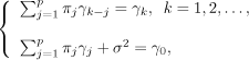

where σ2 is the variance of εt.

PROOF.– For k ≥ 1

In addition

and

Asymptotic correlation: The autocorrelation of (Xt) is defined by setting:

From the first formula of [14.3], we have:

Yet

is then a solution to (E). We deduce for (E) the general solution:

where the ci are constants. Therefore, (Pk) is in general a mix of decreasing exponentials and damped sinusoids. In any case

Partial autocorrelation

DEFINITION 14.2.–

1) Let X, Y, Z1,…,Zk ∈ L2 be centered. The partial correlation coefficient between X and Y, relative to Z1,…, Zk, is defined by:

where X* and Y* are the orthogonal projections of X and Y onto the subspace of L2 generated by Z1,…, Zk.

2) Given a weakly stationary, centered process , its partial autocorrelation (rk, k ≥ 1) is defined as:

with the convention rk = 0 if σ (Xt − X*t) = σ (Xt−k − X*t−k) = 0.

THEOREM 14.2.– If (Xt) is anAR(p), then

PROOF.–

– For k = p, we deduce by projection from [14.1] that

Hence

Since εt ⊥ Xt−p − X*t−p, we have

but by stationarity

therefore

– For k > p, we find:

It follows that

14.2. Moving average processes

DEFINITION 14.3.– is said to be a moving average process of order q (MA(q)) if:

[14.4]

where a0 = 1, aq ≠ 0; εt is a white noise such that .

The expansion [14.4] is unique and, if the roots of (z) = 1 + a1z + … + aqzq are of modulus > 1, we have:

with ∑ |πj| < ∞ and

Therefore,

EXAMPLE 14.2.– If Xt = εt + a1εt−1, |a1| < 1, we deduce that

Autocovariance: A direct calculation shows that

Partial autocorrelation: It is difficult to calculate. For an MA(1), we find:

This type of result is general: (rk) tends to 0 at an exponential rate for all MA(q).

14.3. General ARMA processes

An ARMA(p, q) process is defined by the equations:

[14.5]

which may be symbolically written as:

with ϕpθq ≠ 0, supposing P(a) = 0 and (a) = 0 have no common roots.

If the roots of P and are outside of the unit disk, we have the representations

[14.6]

and

[14.7]

Therefore, (Xt) is a linear process with innovation (εt), and p, q, (ϕj), and (θj′) are unique.

Autocovariance: From [14.5], it follows that

For k > q, we obtain:

which is a Yule–Walker equation (see Theorem 14.1), therefore (γk) has the same asymptotic behavior as the autocovariance of an AR(p).

Partial autocovariance: Relation [14.6] shows that one may approach an ARMA (p, q) process by an MA(q′). Using this property, it may be established that the partial autocorrelation of an ARMA has the same asymptotic behavior as that of an MA.

Spectral density: Let us set:

Using Lemma 10.1 twice, we obtain:

where fY and fX are the spectral density of (Yt) and (Xt), respectively, and σ2/(2π) is the (constant) spectral density of (εt).

Consequently,

This rational form of the spectral density characterizes the ARMA process.

14.4. Non-stationary models

In practice, observed processes more often have a non-stationary part, which must be detected and eliminated to reduce the problem to the study of a stationary process. Some empirical methods were indicated in Chapter 9 (section 9.3). We now present some more elaborate methods.

14.4.1. The Box–Cox transformation

Let (Xt) be a process whose variance and mean are related by an equation of the form

where φ is strictly positive.

We may then stabilize the variance by transforming (Xt). Indeed, if T is a sufficiently regular function, we will have in the neighborhood of EXt:

that is

This (heuristic!) reasoning leads us to choose a transformation T such that

where k is a constant.

For example, if VarXt = c(EXt)2 and Xt > 0, we may choose T(Xt) = log Xt. If VarXt = cEXt and Xt > 0, we choose .

More generally, we may use the Box–Cox transformation:

Then λ appears as an additional parameter that must be estimated.

14.4.2. Eliminating the trend by differentiation

When the trend of a process is deterministic, it may be estimated by the least-squares method (see section 9.3). If it is stochastic, we seek to eliminate it.

Consider, for example, a process (Xt) defined by:

where the εt are i.i.d.

E(Xt|Xt−1,…) = Xt−1 is then the trend and the process

is stationary.

This leads us to define an ARIMA(p, q, d)process as an (Xt) satisfying

[14.8]

where P and are polynomials of respective orders p and q, with roots that lie outside of the unit circle, and d is an integer.

(Xt) may then be interpreted as an ARMA process such that 1 appears among the roots of the autoregression polynomial.

Since we cannot invert P(B)(I−B)d to determine Xt as a function of the εt−j, we require p + d initial values: X_t0−1, X_t0−2,…, X_t0−p−d that determine X_t0. When all the starting values are eliminated, the process reaches its cruising speed, and (I − B)d Xt coincides with an ARMA(p, q) process.

14.4.3. Eliminating the seasonality

If (Xt) has a trend, and period S, we may envisage a model of the form:

where

with dP2 = P and d2 = .

(Xt) is then said to be a SARIMA (p, q, d; P, Q, D)S process.

The SARIMA (0,1,1;0,1,1)12 model is widely used in econometrics, and is written as:

14.4.4. Introducing exogenous variables

The previous models have the drawback of being closed: they only explain the present of Xt from its past values. It is more realistic to allow exterior variables to play a role: for example, the consumption of electricy is related to the temperature.

Then, letting (Zt) be the process associated with an “exogenous” variable, we may envisage the ARMAX model defined by:

where P, , and R are polynomials.

More generally, we may consider the SARIMAX model obtained by introducing an exogenous variable into a SARIMA process. For details, we refer to the bibliography.

14.5. Statistics of ARMA processes

14.5.1. Identification

For simplicity, we suppose that the initially observed process is an ARIMA (p, q, d) model. To identify d, we may note that if d is strictly positive, the observed random variables are strongly correlated.

For example, if Xt = ε1 + …+εt,t ≥ 1, the correlation coefficient of (Xt,Xt+h) is written as:

thus it tends to 1 when t tends to infinity with h fixed, or faster than h.

The random variables X1,…,Xn being observed, the empirical correlation coefficients are given by:

If vary slowly with h, and are not in the neighborhood of zero, then it is recognized that the model is not stationary, and we consider the differentiated series

We then consider the empirical correlation coefficients of (Yt) and we may continue to differentiate. It is advised to choose d ≤ 2, as each differentiation leads to a loss of information.

We are now in the situation where the observed process (Xt) is an ARMA(p, q): we identify (p, q), or more precisely, we construct an estimator of (p, q).

Among the various methods that have been proposed, we choose two:

1) The Corner method (Beguin, Gouriéroux, Monfort)

This method is based on the following theorem.

THEOREM 14.3.–Let (Xt) be a stationary autocorrelationprocess (ρt). Consider the determinants

and the matrix M = (Δij)1≤i,j≤k (Xt) is then an ARMA(p, q)process (where p < k, q < k) if and only if M has a “corner” at the intersection of the qth line and the pth column:

PROOF.–See [GOU 83]. The method consists of forming the that allow the construction of an estimator , then seeking a “corner” in . For details of the implementation of this method, we refer to [GOU 83].

2) The Akaike criterion

This is based on the interval between the true density, i.e. f0, of the observed vector (X1,…, Xn) and the family of densities associated with the ARMA(p, q) model. The chosen risk is the Kullback information:

The estimators of I that have been proposed are of the form:

where is the maximum likelihood estimator of σ2 when (Xt) is a Gaussian ARMA(p,q) process, and (un) is a sequence which depends only on n.

Then, = argmin . If un = log n/n where un = c log log n/n with (c > 2), then is an estimator that converges almost surely to (p, q) when n → ∞.

COMMENT 14.1.– Before using the methods that we have just outlined, it is useful to calculate the , and to construct some estimators of the partial autocorrelations. The results of sections 14.1 and 14.2 then provide the following empirical criteria:

– If becomes small for h > q, the model is an MA(q).

– If becomes small for k > p, it is an AR(p).

– If and decrease slowly enough, the model is mixed.

14.5.2. Estimation

The observed process is now assumed to be an ARMA(p, q), where p and q are known. It is necessary to estimate the unknown parameter:

where ϕj are the coefficients of the polynomial ρ, θj are those of , and σ2 is the variance of εt.

When (Xt) is Gaussian, we may estimate η using the maximum likelihood method. This method has the advantage of providing estimators with minimal asymptotic variance, but its implementation is delicate, as the likelihood is complicated. In the context of an MA(q), we have:

therefore (X1,…, Xn) is the image of the Gaussian vector (ε1−q,…, εn) by linear mapping. This remark allows us to explicitly give the variance since the εt are i.i.d. with distribution .

In the general case, one may obtain an approximation of the likelihood by approaching (Xt) with an MA(Q′).

If the process is an AR(p), it is preferable to use the conditional maximum likelihood method.

The process is of the form:

Denote by f the density of (X1−p,…, X0) and consider the vector (X1−p, …, X0, ε1,…, εn) with density:

The change of variables , n, let us obtain the conditional density g of (X1,…, Xn) given (X_1−p,…,X₀ ):

Supposing the random variables (X1−p,…, X0, X1,…, Xn) to be observed, we obtain the conditional likelihood equations:

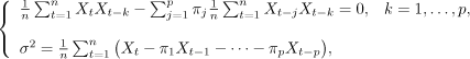
hence the estimator .

Note that these equations are obtained from the Yule–Walker equations [14.3] by replacing the autocovariances with empirical autocovariances.

From this remark, it may be shown that even in the non-Gaussian case,

14.5.3. Verification

The previous operations allow the construction of , and , which completely determine the model.

To verify the suitability of the model to the observations, we define the residues by:

where and are the estimators of the polynomials P and , respectively.

To test the independence of the , we consider the empirical autocorrelations associated with the observed , and we set:

Then, if K > p + q, it may be shown that Qn converges in distribution to a χ2 with K − p − q degrees of freedom, whence the Box–Pierce test with critical region

where, if Z follows a χ2 distribution with K −p − q degrees of freedom,

This test is of asymptotic size α.

If the model is revealed to be inadequate, the identification procedure must be re-examined.

If several models survive the verification procedure, we choose the model that has the best predictive power, i.e. the model for which the estimated prediction error is the smallest.

14.6. Multidimensional processes

The study of multidimensional processes lies outside the scope of this book. We will only give some indications.

We will work in , equipped with its Borelian σ-algebra (the σ-algebra generated by open balls) and with its Euclidian structure (scalar product , norm .

Let be a sequence of random variables with values in . Supposing , the expectation X_t = (X_t1 , . . . , X_td ) is defined by setting

The cross-covariance operator of (Xs,Xt) is the linear map from to defined by is called the covariance operator of Xt (written C_Xt).

The process (Xt) is then said to be stationary if EXt does not depend on t and

EXAMPLE 14.3: WHITE NOISE IN .– Let be a sequence of random vectors with values in such that , and

This is a stationary process.

EXAMPLE 14.4: MA(∞).– Letting (εt) be a white noise with values in , we set:

[14.9]

where the aj are linear operators from to such that with ; series [14.9] is then convergentin mean square in :

and the process (Xt) is stationary. Under certain conditions, (Xt) becomes a d-dimensional ARMA process (see [GOU 83]).

Extension to infinitely many dimensions is possible, notably in a Hilbert space (see [BOS 07]).

14.7. Exercises

EXERCISE 14.1.– Show that if (Xt) is a d-dimensional stationary process, its coordinates are stationary.

Explain why the converse is not necessarily true.

EXERCISE 14.2.– (AR(1)) Let (εt) be a white noise in and ρ be a linear map from to . The process (Xt) is defined by setting:

[14.10]

where .

1) Show the equivalence of the following two conditions:

2) Assuming i) to be satisfied, show that [14.10] has one unique stationary solution given by:

where the series converges in quadratic mean in .

3) Determine EXt. Show that C_{Xt−1, εt} = 0 and deduce the relation:

where ρ′ is the transpose of ρ.

4) Establish the relation CX_t−1 ,X_t = ρC_X0.

EXERCISE 14.3.– (AR(1)) Consider the AR(1) defined in the previous exercise. We observe X1,…,Xn and seek to estimate the parameters of this process.

1) One estimator of m is defined by setting . Show that the series is convergent, and that

2) Supposing m = 0 and is invertible, use the relation to construct an empirical estimator of ρ. Study its convergence in probability.

EXERCISE 14.4.– (AR(1)) Consider the AR(1) model:

where (εt) is a Gaussian white noise with variance σ2.

We observe X1,…, Xn and wish to estimate θ = (ρ,σ2).

1) Calculate the covariance matrix of (X1,…, Xn) and deduce the expression of the density fn(x1,…,xn;θ).

2) Writing f(xt|xt−1; θ) for the density of Xt given Xt−1 = xt−1, show that

3) Determine the conditional maximum likelihood estimator of θ by maximizing

Compare this estimator with the least-squares estimator.

4) Study the convergence of .

EXERCISE 14.5.– Let be a real, centered, regular, weakly stationary process. Supposing the autocorrelation (ρj,j ≥ 0) of (Xt) satisfies the following property:

show that (Xt) is a moving average of order q.

EXERCISE 14.6.– Let be a white noise and ρ be a real number such that |ρ| > 1. We set:

[14.11]

1) Show that this series converges in quadratic mean.

2) Show that (Xt) is the unique stationary solution to the equation

[14.12]

3) Calculate Cov(Xt−1, εt). Is [14.11] the Wold decomposition of the process?

4) Determine Cov(Xs, Xt).

5) Setting

determine the spectral density of (ηt). Deduce the Wold decomposition of (Xt).

6) Now, supposing ρ = 1, calculate Var(Xt+h − Xt), h ≥ 1. Show that, if [14.12] has the stationary solution (Xt), we have:

Deduce that such a solution does not exist.

7) Treat the case where ρ = −1.

EXERCISE 14.7.– Let be a white noise. Consider the moving average

1) Establish the relation:

2) Deduce

where the limit is in quadratic mean.

3) Show that (εt) is the innovation of (Xt), while the root of the associated polynomial has modulus 1.

EXERCISE 14.8.– Let be a weak white noise, and θ ≠ 1. We set:

1) Compute the covariance function of . Deduce that it is stationary, and calculate its spectral density.

2) Show that if |θ| < 1, then . Deduce in this case the Wold representation of .

3) Show that if |θ| > 1, then . Is Xt = εt− θεt−1 the Wold representation of the process?

EXERCISE 14.9.– Let be a weak white noise with variance σ2. Supposing there exists a stationary process in the weak sense, which satisfies the equation:

determine its Wold representation and its spectral density.

---

1 For the definitions of and see Chapter 10.