
CHAPTER 7
Manufacturing Engineering
Manufacturing Engineering facilitates the manufacturing function. In other words, Manufacturing is the executor, whereas Manufacturing Engineering is the enabler. The relationship between Manufacturing Engineering and Manufacturing is analogous to the relationship between Marketing and Sales. Typical Manufacturing Engineering activities include designing production lines, reducing the manufacturing cycle time of existing products, manufacturing tooling, reducing setup time, improving process capability, etc. The focus for Manufacturing Engineering features in Oracle Applications has increased in recent releases, especially in the areas of flow line design. This chapter presents the theoretical background in the beginning and then describes the features in Oracle Applications that support the Manufacturing Engineering function.
Process Layout
A process layout organizes production resources by processes. The products that are being produced in the process layout are moved to the appropriate process in a predefined sequence. For example, if an automobile wheel needs to go through the grinding, plating, and painting processes, wheels will be moved to these processes one after the other in an appropriate batch size.
In Oracle Applications, you can model these processing centers or work centers as departments, and assign the individual resources to these departments in the appropriate number. These departments and resources are then included in the routings of the assemblies that need to be processed in those departments. Departments and Resources are covered in Chapter 4.
Product Layout
A product layout organizes production resources by the production sequence of a family of products. The resources are organized in such a way that all the products that are being produced follow a flow pattern before reaching the final state. Generally, it is not very economical to have a product layout for just one product—so typically, a product layout is designed for a family of products.
In Oracle Applications, you can model a product layout as a repetitive production line or a flow line. Repetitive lines can be defined using the Production Lines form. Although there are many features in planning and manufacturing execution that support repetitive manufacturing, there aren’t many manufacturing engineering features. The bulk of the manufacturing engineering features that Oracle provides deals with designing lines for flow manufacturing; it is flow line design that is the focus of this chapter.
Line Layout
A flow line is a collection of machines and/or assembly workstations. The resources in a line are arranged to address one or more constraints—for example, distance traveled by the product or the space occupied by the machines. Some lines might be U-shaped, whereas another might be organized as a straight line to satisfy these constraints.
Final Assembly Line
A final assembly line produces the assembly that is shipped to the customer. The demand for the final assembly is independent in nature. In a pull-based system, the final assembly line is communicated with the change in demand scenarios. The final assembly line reacts to this change, whereas the feeder lines and the replenishment processes react to the change in requirement from the final assembly line.
Feeder Lines
A final assembly line can potentially have many feeder lines. Although there is not much difference in the way they are designed, feeder lines produce subassemblies or components that continuously feed the final assembly line that produces the final product at the required rate and time.
In Oracle Applications, there are two types of feeder lines, attached and detached. An attached feeder line produces first level components or phantom items. A detached feeder produces subassemblies that have second-level BOM on the parent assembly.
Product Synchronization
Product synchronization shows the relationship between the individual production processes that produce a product. This final assembly line forms the trunk of this tree diagram, while the various feeding lines connect to this final assembly line at various points of the tree. In the world of flow manufacturing, a finished assembly is viewed as a pile of parts and a sequence of steps. Establishing the product synchronization enables you to get a high-level view of the manufacturing process flow and is one of the very first steps in designing a line.
Line Design Process and Factors
Each production line is unique. Even within a production line, one product might undergo a significantly different set of operations from another product. Yet, it is possible to follow a standard set of steps in building a highly flexible and responsive line. Figure 7-1 outlines these high-level steps. The rest of the chapter talks about these steps in detail and explains the various features within Oracle Applications that can be applied at these steps.

FIGURE 7-1. High-level steps in building a flow line
The first step in building your line is to identify the set of products that can be potentially produced by this line. Product families were covered in detail in Chapter 4. When you have identified your product families and the individual products within each product family, define all the process steps and events for each product. You can also calculate the approximate total product cycle time (covered in the section “Total Product Cycle Time”) after you define the various processes for each product.
Define a set of events from the manufacturing viewpoint and group them into line operations in such a way that the operation cycle time doesn’t exceed the takt time (covered in the section “Takt Time”), at the designed daily rate (covered in the section “Designed Daily Rate”) of the product. As a rule of thumb, you can calculate the minimum number of line operations before you proceed with the design process (the formula is presented in the section “Number of Line Operations”). While establishing the sequence of events, the thought process should follow the natural flow of the product. But also keep in mind that it’s important to look at the flow creatively to gain maximum benefit. For example, one auto manufacturer reportedly installs one tail light at one point on the line, and the other much farther downstream—the movement of that unit of work (installing one tail light) was found to produce a better balanced line than installing both at the same time.
After defining an approximate grouping, generate the mixed model map and analyze the output (mixed model map is covered in section “Mixed Model Map”). Continue to regroup the work events until the desired results are achieved. When you are satisfied with the results, you have to document the different output levels of the line for each product within the product family and the number of labor resources that are required in each of those scenarios.
Before delving deep into the line design process, let us examine some of the important factors that have an impact on the line design process. Some of these factors are not calculated by Oracle Applications currently. They are mentioned here because they have a great deal of influence to the line design process.
Designed Daily Rate
The Designed Daily Rate (DDR) represents the designed capacity of a line. DDR represents the maximum output levels of the line at any time. It is very hard to operate at an output level that is higher than the DDR for an extended period of time. DDR is calculated using this formula:

The DDR is part of the contract that is established between Marketing and Manufacturing. Currently, the DDR for each product has to be calculated manually.
Flow Rate
Flow Rate represents the rate at which production should progress on an hourly basis. Flow rate can be calculated using this formula:

The effective work hours are the shift work time that is adjusted for allowances, such as breaks, maintenance, or efficiency. Flow rates are useful in line design as well as monitoring line performance on an hourly basis. Currently, the flow rate for each product has to be calculated manually.
Takt Time
Takt is a German word that implies “drumbeat” or “rhythm.” In the context of flow manufacturing, Takt Time represents the ideal time for each operation during the production of a product. The line (and each operation) must complete one assembly when one unit of takt time elapses to satisfy the market requirements; if each operation takes exactly the takt time, the line will be perfectly balanced. If some operations take longer than the takt time, you’ll be building bottlenecks; if some operations take less than the takt time, you won’t be fully utilizing those resources.
Takt time is the inverse of flow rate multiplied by 60 to get the time in minutes. Takt time can be calculated directly using this formula:

The Mixed Model Map calculates takt time for a group of products, using this formula:
![]()
In principle, the takt time represents the targeted work content time at each line operation. So, the work events are grouped into line operations that are approximately equal to the takt time, but should never exceed the takt time. Note that this is the takt time at the DDR. If you operate at a rate that is lower than the DDR, your takt time will increase.
Number of Line Operations
When you have the takt time and the work content, you can calculate the approximate number of line operations that are required in order to meet the daily demand using this formula:
![]()
The # of line operations gives you an idea as to how many workstations might be required in the line. For example, if the manufacturing lead-time is 120 minutes, and if the takt time at the designed daily rate is 6.7 minutes, the number of line operations is approximately 18. Currently, the number of operations has to be calculated manually.
Operation Times
The operation times can be calculated for the events, processes, and line operations that are available in your flow routings. The operation time calculations are based on the resources that are available in each of the events.
The calculated labor time for an event is the sum of scheduled and unscheduled labor usage rates in the event. The calculated labor time for a process or a line operation is the sum of the calculated labor times of all the events that form the process or line operation. Events with a lot basis will temporarily be converted to item basis for this calculation. The calculated machine time is similar to calculated labor times, except that the system includes the scheduled and unscheduled machine times in the calculation.
The calculated elapsed time for each event is the sum of the non-overlapping scheduled labor and machine usage rates for each event. The calculated elapsed time for a process or a line operation is the sum of the elapsed times of all the events that form the process or line operation.
The resources that will be included in these three lead-time calculations are illustrated by Figure 7-2 (resource type of L indicates labor resource and M indicates machine resource).
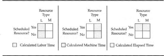
FIGURE 7-2. Resources that are included in Operation Time calculations
NOTE
Elapsed time will not include scheduled resources that overlap with other scheduled resources. For example, if you have an operator who spends 1.5 minutes of scheduled time in an event, which also has a machine that runs for 4 minutes after the operator, the elapsed time for the event is 5.5 minutes. On the other hand, if the machine doesn’t have to wait for the operator, the elapsed time would be 4 minutes.
To calculate the operation times for an assembly, choose Tools I Calculate Operation Times.
Total Product Cycle Time
When you design an item, you identify the steps in manufacturing the item as processes in the flow routing. The processes in turn are a collection of events. Using these processes, you can calculate the Total Product Cycle Time (TPCT) of an item. The TPCT is the longest lead-time through the production process, considering all the feeder lines.
If you create subassemblies on a detached feeder line (standard subassemblies in the second level of a BOM), you would use feeder line sync and perform a work order-less completion at the end of that line. This is covered in detail in Chapter 16. The work content on the feeder line would not be part of the TPCT for the final assembly.
An attached feeder line (single level on the BOM or a second-level phantom) is counted in the TPCT. This is illustrated by the example in Figure 7-3. The feeder’s feeding operations 10 and 30 are attached feeders and will be included in the TPCT calculation of the assembly, whereas the feeder that feeds operation 20 is a detached feeder and will not be included in the TPCT calculation.

FIGURE 7-3. TPCT calculation with attached and detached feeders
The system always calculates TPCT from the back. For example, in Figure 7-3 the two paths that will be considered for TPCT calculations are 40-30-301-302-303304 (Path #1) and 40-30-20-10-101-102-103 (Path #2). The Path 40-30-20-DF30-DF20-DF10 will not be considered since that path includes a detached feeder line. The lead-time for Path #1 is 140 minutes, and the lead-time for Path #2 is 120 minutes. So the TPCT for the assembly is 140 minutes.
To calculate TPCT for an assembly, choose Tools I Calculate Total Cycle Time. Alternatively, you can enter a Total Cycle Time manually as well.
CAUTION
The TPCT is calculated using the rolled up elapsed time of each operation (covered in the previous section). You can enter the elapsed times manually for each operation, but these will not be included in the TPCT calculation.
You can choose to include either processes or line operations in the TPCT calculation. Before designing the line, you can use processes to calculate the TPCT to get an approximate TPCT. After you complete your line design, you can recalculate the TPCT that is based on the line operations.
NOTE
When you make changes to your flow routing by adding or removing events, processes, and line operations, the lead times and total cycle time are not recalculated automatically. You have to use Tools I Calculate Total Cycle Time and Tools I Calculate Operation Times to recalculate these times.
After you calculate the TPCT in the flow routing and the Takt Time in the mixed model map, set the value of TPCT for the Fixed Lead Time item attribute and the value of the takt time for the Variable Lead Time item attribute. The planning processes will use these lead-times. The implied understanding is that you will take the time that is equivalent to the TPCT of the product to roll out the first item, and it will consume one takt time for every product thereafter.
Line Output Levels
The production line is designed for the maximum capacity (the designed daily rate). But the line will not operate at this maximum capacity all the time. The line output will depend on the market requirements at the time. This is a fundamental principle of flow manufacturing—you produce no more or no less than what is required.
This is achievable only if you have flexible resources. The strategy is to invest in machine resources such that the machine cycle time is balanced enough to produce the item at the designed daily rate. At the same time, develop flexible labor resources that can work on the different operations in the same line or potentially can work in other lines. This flexibility cannot be achieved overnight; operator training and a flexible incentive system (which takes the number of skills possessed by each employee into consideration) are two important means in producing flexible labor. In this section, we take an example and illustrate how you can react to demand fluctuations.
Manufacturing Engineering will design the line to operate at the maximum capacity, document the alternative output levels and the corresponding resource requirements, and hand over the line to manufacturing.
As demand moves up and down within the previously negotiated limits, line managers have to redeploy their labor resources to manage the supply. To illustrate this, let us take a simple example, where you are producing one assembly in a line. Table 7-1 lists the operations of this assembly on the line that produces this assembly. The table lists each operation and the composition of labor and machine time in the operation. For the sake of simplicity, we assume that all the labor and machine resources in each operation are scheduled. So, the total elapsed time is the sum of the labor and machine times. With this background, let us investigate two demand scenarios with which this line might be operated.

TABLE 7-1. Summary of Line Operation Times for the Example
Scenario I
In this scenario, the line is required to produce 260 assemblies per day. The takt time for this output level is 5.54 minutes. Figure 7-4 shows one possible way of deploying your labor resources to achieve this level of output. The first resource handles operations 10, 20, and 30; the second resource handles operations 40, 50, and 60; the third resource handles operations 70, 80, 90, and 100; and the fourth resource handles operations 110, 120, and 130.

FIGURE 7-4. The Line operated with four persons
To analyze the output levels of this line, you need to consider two factors—the operational cycle time for each operation and the load on each labor resource. If you quickly skim through the operational cycle time column in Table 7-1 and the total time taken by each labor resource in Table 7-2, you’ll notice that except operation 40, all the times are either equal to or less than the line takt time. To balance this line, you might place some in process kanbans after operation 40 to act as a buffer between operations 40 and 50. With this configuration, the line can deliver approximately 262 assemblies per day under normal operating conditions.

TABLE 7-2. Labor Resource Deployment Details for Scenario 1
Scenario 2
In this scenario, you are required to produce 240 assemblies per day. That works out to a takt time of 6 minutes. Figure 7-5 shows one possible way of deploying your labor resources to achieve this level of output. Note that this layout only uses three labor resources as compared with the layout in Figure 7-4, which uses four labor resources. The first resource handles operations 10, 20, 120, and 130; the second resource handles operations 30, 40, 100, and 110; and the third resource handles operations 50, 60, 70, 80, and 90. In this scenario, the labor resources are flexed across a higher number of operations and this might involve additional fatigue. This fatigue will have to be factored into the operation cycle times appropriately.

FIGURE 7-5. The Line operated with three persons
On quickly skimming through the operational cycle time column in Table 7-1 and the total time taken by each labor resource in Table 7-3, you’ll notice all the times are either equal to or less than the line takt time. With this configuration, the line can deliver approximately 240 assemblies per day under normal operating conditions. Also note that the in process kanban after operation 40 is no longer necessary, since the operation cycle time is now less than the takt time.

TABLE 7-3. Labor Resource Deployment Details for Scenario 2
The mixed model map (covered in the section “Mixed Model Map”) provides you with the capability to analyze the operation times and identify the bottleneck operations; it also calculates the in process kanban that is needed as a buffer. The actual resource deployment is not known at the time of designing the line. As you increase or decrease the number of labor resources deployed in the line, the line output will increase or decrease correspondingly. These scenarios need to be captured during the line design phase along with the number of labor resources and the corresponding output level in a table that is shown in Table 7-4. When the output requirements change, you should be able to step up or step down your output from the current levels.

TABLE 7-4. Labor Resource Deployment Scenarios
To record these alternative resource deployment scenarios, you should define multiple representations for the same labor resource. In Table 7-4, at the designed daily rate, there are five operation groupings. So, you will have to define at least five resources—W12-1, W12-2, W12-3, W12-4, and W12-5. When you have this, you can define Alternate Routings, with names such as 5Person, 4Person, etc., and record these alternative resource deployments. Using the Switch to Primary feature that was discussed in Chapter 4, you can make one of these Alternate Routings active at any point in time, depending on the required output level.
NOTE
The multiple representation of the same labor resource need not be product or line specific. For example, W12-1… W12-5 can be used in other products that are produced in other lines as well.
Using the line designer (covered in the section “Graphical Line Designer”) and the mixed model map, you can create alternative scenarios that meet the two important objectives of a flow line—to achieve a takt time for an output level that is equal to the designed daily rate and to design the operations in such a way that you can change the output levels easily by flexing your labor resources.
Designing Lines
A highly responsive line should be designed after taking the peak demand into consideration. The designed daily rate thus represents the peak demand that is agreed to by everyone. Although the line is designed for this peak demand, the line is not required to operate at this peak demand. Typically, the line can operate anywhere between the peak capacity and 50 percent of this peak capacity, by flexing the resources. In certain cases, the line might be flexible enough to operate at significantly lower capacities, but it might not make economical sense to operate a line at these levels for long. During the line design process, you will have to consider these alternative capacity scenarios and plan alternative resource deployments. For example, if you operate the line with five labor resources, you might be able to achieve a flow rate of 20 per hour, whereas if you use four labor resources, you might achieve 15-17 per hour. These different scenarios can be modeled as Alternate Routings during the line design phase. With sufficient notice, manufacturing can step up or step down the line output. In this section, we discuss the features in Oracle Applications that can be used for designing and balancing your flow lines.
Defining Flow Lines
You define flow lines in the Lines window, which is shown in Figure 7-6. Name the line and specify the line start time and stop time to indicate the hours of operation of the line. For 24-hour lines, set the stop time equal to the start time. Set the line lead-time as routing based, so that the line lead-time can be dynamically calculated based on the product routings.

FIGURE 7-6. Define flow lines and specify flex fences
The Maximum Hourly Rate and Minimum Hourly Rate enable you to specify the boundary conditions for the line. The maximum hourly rate is equal to the designed daily rate divided by the effective hours of operation of the line, if the line produces only one product.
The minimum hourly rate can be equal to 0, although that might not be economical in reality. If the line produces more than one product, you should estimate the rates for the line considering the demand for all the products.
Tolerance Fences
Marketing and Manufacturing establish an agreement that details the extent to which manufacturing can either step up or step down their output levels and the amount of notice (in terms of days) for the change in output level. This agreement is represented as tolerance fences in Oracle Applications. Tolerance fences provide the marketing team with the flexibility to quickly respond to customer demand fluctuations. If the line produces more than one product, you should estimate the tolerance fence for the line considering the demand for all the products.
You can specify these tolerance fences in the Tolerance Fences window that you can access by clicking the Tolerance Fences button in the Production Lines form. The scheduling tool will use the flex fences to consider excess demand, based on dates and the corresponding expanded capacity. For example, you can go over 20 pecent of the standard capacity with 15 days notice.
Graphical Line Designer
The Graphical Line Designer enables you to visually design a flow line. You can add standard operations, processes, and events to an item’s routing by dragging and dropping the appropriate icons. The designer consists of two panes—the tree hierarchy pane and the graphical network pane, as shown in Figure 7-7.

FIGURE 7-7. Design lines using the drag and drop of features of the Graphical Line Designer
The Tree Hierarchy Pane
The tree hierarchy pane (left pane) enables you to switch between two views—Item Routings view and Template Routings view using the tree tabs on the left side of the pane. The Item Routings tab displays all the items that are associated with the line. The Template Routings tab displays all the product families that can be used as a template for creating new routings.
When the graphical line designer is first brought up, the Item Routing tree tab is selected on the left pane and the tree is collapsed. When you select an item on the left pane, you will see a graphical network of line operations on the graphical network pane (covered in the next section). The View by drop-down list enables you to view the line items either as a list or as a list that is organized by product family.
Select the top-level node Item Routings and press the right mouse button on the node. Choose New from the pop-up menu to create a new routing. This will bring up the Add Item Routing window. From this window, you can create a new routing, copy the routing from another item or a template, or assign a common routing for this item.
If you want to access the routing details of an item, navigate to that item and press the right mouse button. Choose Routing Details from the pop-up menu to bring up the Routing Details window. From here, you can view or update the routing information.
To view or update the routing revisions, choose Routing Revisions from the pop-up menu. Choosing Items will bring up the Master Items window, from which you can define new items. You can also view the bills or indented bills of the selected node by choosing the appropriate menu option.
If you are on an Alternate routing in the tree navigator, you can make that routing the Primary routing by choosing Tools I Switch to Primary. Switching between alternates and primary was covered in Chapter 4.
The Graphical Network Pane
The graphical network pane (right pane) displays the routing details of the item that is selected on the left pane. This pane is divided into four tabs—Line Operation (network view), Line Operation Tree (tree view), Process (network view), and Process Tree (tree view).
When you are on the network view tabs (either Process or Line Operation), you see a toolbar that contains five icons. The Connector icon lets you create links between line operations or between processes, depending on which tab you are in. The second icon is a selection tool that enables you to move existing line operations or processes. Process and Line Operation are the third and fourth icons, and they enable you to add processes and line operations in the Process and Line Operation tabs, respectively. These icons will be enabled only if you are on the correct tab. The fifth icon enables you to add events to the routing.
To create a line operation, process, or event, choose the appropriate icon in the toolbar and click on the graphical network canvas. If you have selected the operations icon, clicking on the canvas will bring up the Line Operation window, where you can either create a new one or select an existing operation. The process and event icons behave in the same way.
To define a network connection, select the Connections icon. Click the first operation or process and drag onto the target operation or process to create a network connection between them. This will bring up the Network Connection window, where you can identify the Transition Type and the Planning Percent. The possible values for transition type are Primary, Alternate, and Rework. The planning percent is the percentage of product that follows this network path.
When you are on the Tree View tabs (Line Operation Tree and Process Tree), you see another toolbar that has four icons and two drop-down menus. The first three icons enable you to view the line operations/processes in three tree styles—Vertical style, Organizational Chart style, and Interleaved style. The fourth icon toggles the view of the event/line operation/process times in the tree view. The first pull-down menu enables you to switch between viewing system calculated operation times and user entered operation times. The second pull-down menu enables you to view the current, future and current, or all events on the routing.
When you are on the tree views, the last node will be named as Un Assigned Events. This node will enable you to access all the events that are available in the routing, but haven’t been assigned to any process or line operation in the routing.
You can explode the nodes of a tree and assign events to each process or line operation by dragging and dropping events from the Un Assigned Events node. This feature is useful during line design. Potentially, you will have to iterate between generating the mixed model map and dragging and dropping events between line operations several times.
On the graphical network pane, you can right-click any of the icons (in the network views) or any of the nodes (in the tree views), which will bring up a pop-up menu with five choices: Cut, Paste, Delete, Properties, and Standard. Cut enables you to remove an operation, process, event, or connection and store this information on the clipboard. Paste enables you to paste an icon that has been previously put in the clipboard. Delete permanently removes an operation, process, event, and the associated connections. The Properties menu takes you to the details window of the relevant operation, process, or event. Standard enables you to access the Standard Line Operations, Standard Processes, or Standard Events window, depending on the type of icon on which you’re right-clicking.
While designing lines, you will try out various combinations of resources and events to achieve your design objectives. When you change the operation compositions, you generate the mixed model map and review the composition of each operation in terms of the machine and labor time and the total time. You can generate the mixed model map from the line designer using Tools I Mixed Model Map.
Mixed Model Map
The Mixed Model Map (MMM) is a powerful tool that can help you in identifying imbalance problems. The MMM takes a form of demand and a product mix and provides you with a recommendation for smoothing your line operations or processes.
Mixed Model Map Parameters
To generate the MMM, you provide a demand source which can be one of four demand types—Forecast, Master Demand Schedule, Master Production Schedule, or Flow Schedule. You also optionally provide the product family that will be produced by this line; this will restrict the calculations to only the specified product family in the demand stream and is useful if your demand includes products not produced on the designated line. Specify the start date and end date of the demand period. The Demand Days will be calculated as the difference between the start date and end date. The effective work hours per day can be specified in the Hours per Day field. Use the boost percentage to increase or decrease your demand during the MMM generation.
The MMM can be generated either for line operations or processes. The output can be sorted by the Display Sequence or the Operation/Process Code using the Sort Order field. You can choose to include either the rolled up time or the manually entered time in the MMM calculations. The process can recommend the in process kanban either for the process/operation or for each machine. Specify the IPK recommendation level using the IPK Value field. The Time UOM enables you to view the time information in the map in hours, minutes, or seconds. When you specify the appropriate values in the MMM parameters form, press the Generate button to generate the MMM output.
Mixed Model Map Output
This MMM generation process takes these inputs and identifies the total demand for all the products in the family. For this total demand, the resources required for each of the line operation is calculated. Additionally, the process also calculates the in process inventory that is required to keep the line in balance. Figure 7-8 shows a mixed model map output.

FIGURE 7-8. Generate mixed model map for the line and compare it with the baseline
Resource Recommendations
The MMM calculates the process volume for each operation/process. This is the number of units that will pass through the operation or process. For example, an operation that is used by only some products on the line will have a lower process volume than an operation that is used by all products; an operation that is repeated in rework loop will have a higher process volume than one that is not repeated. The MMM uses this process volume to weight the operation times that were covered earlier to calculate the three weighted times—Machine Weighted Time (MWT), Labor Weighted Time (LWT), and Elapsed Weighted Time (EWT). The machines and labor that are needed at each operation or process are calculated by dividing the MWT and LWT, respectively, by the operation takt time.
The machines and labor assigned in each operation are the total number of resources in the department that the events are assigned to. For example, an operation LO1 comprises events E1 and E2. E1 uses a machine resource called M1 from department D1, and E2 uses a machine resource called M2 from department D2. D1 contains four M1s, whereas D2 contains five M2s. The machines assigned for LO1 will be the sum of M1 s and M2s in departments D1 and D2—in this case, 9.
CAUTION
If the same resource (machine or labor) is used in multiple events, the assigned resources will be overstated. In the previous example, if E2 also used the machine resource M1 from department D1, the machines assigned for LO1 would have been 8.
The in process kanbans needed at each operation depend on the extent by which the EWT of the operation exceeds the line takt time. For example, if the line takt time is 6 minutes and the EWT is 8 minutes for an operation, the amount of inventory that is required after this operation is approximately 25 percent of the day’s requirement.
Takt time for assigned (ATAKT) gives you an idea as to how much time will a process/line operation consume if it utilizes all the assigned resources. ATAKT is equal to the EWT divided by the number of people assigned to the operation.
Because absolute synchronization between all the operations is not likely, the next step is to identify the operations that cause line imbalances and solve the imbalance problem. The first time you generate the MMM, the likelihood of seeing fractional resource requirements in every operation is very high. As already noted, line balancing is an iterative process. In MMM, you have a tool, with which you can iterate faster.
The first steps in reducing the imbalances is to regroup your events using the graphical line designer and generate the MMM again. When you reach a point where further optimization might not be practical, you have a few alternatives in solving the remaining problems, depending on the type of resource—machine or labor.
Machine Imbalances
The first alternative is to try to reduce the machine cycle time at the operation that is causing the imbalance. You might reduce the cycle time using various engineering techniques, or you might be able to shift certain processing steps to downstream or upstream machines. In the latter case, you would regroup the respective line operations with the new set of events using the line designer.
The second option is to invest in new machines that can meet the additional requirements, although they give rise to questions on where will they be positioned in the line and the additional space requirements before going through a rigorous capital expenditure review process.
The third option is to build in process inventory after the constrained resource called In Process Kanbans (IPKs) by operating the constrained resource for extra time or shifts.
Labor Imbalances
Labor imbalances can be adjusted by moving some of the labor-intensive events to downstream or upstream operations. In cases where this is not possible, you have to build IPKs by overtime operations of the constrained labor resource or hire additional resources and increase the resource count in the appropriate department.
Another option is to evaluate converting the labor time to machine time if possible.
Operating with Baselines
When you generate the MMM, you can save the results as a baseline for future comparison. You can have one saved baseline for each line or product family combination. To save the generated map as a baseline, choose Tools I Save as Baseline. To query a saved baseline for comparison, choose Tools I View Baseline.
Operational Method Sheets
A standard operation within Oracle Applications typically contains all the events that would be available in the operational method sheet(s) for the operation. Create an operational method sheet for each of the line operations and attach the method sheet as an attachment to the line operation.
In operations involving multiple events, each of the individual pages within the operational method sheet typically corresponds to an event. In such cases, you can attach the page(s) to the corresponding event. Figure 7-9 shows a sample operational method sheet.

FIGURE 7-9. Operational method sheets
NOTE
Operational Method Sheet is also referred to as Operation Standard or Standard Operation in some manufacturing text books. In Oracle Applications, standard operation is different from the operational method sheets.
Building Quality into the Process
It takes a lot of effort to produce quality parts all the time. Stringent quality control and assurance methodologies need to be put in place to achieve high levels of quality. It is important to design a product and the corresponding production processes in such a way that these high quality levels are easily achieved. The following sections discuss some of the online quality control methods that can be designed as a part of the line design process. Chapter 19 covers a complete discussion of Oracle Quality.
Pre-Operation Inspection
When an assembly becomes defective in the middle of a production process, significant resource wastage occurs if the defective assembly is processed farther in the production process. To prevent defective assemblies from moving upstream, you can define standard pre-operation inspection steps and include these steps in your work events. To guide the operators visually, these steps are included as inspection steps in the operational method sheets.
Control Charts
You identify the critical characteristic that needs to be controlled and develop a control chart using Oracle Quality. If necessary, you can create a pre-control chart that can be used by the line operators to monitor the line quality. The line operator is advised on the conditions in which he should raise the alarm. When irregularities are identified from the control chart, the line is stopped until the problems are corrected.
Quick Changeover
Most manufacturing activities involve setup. You can perform some form of setup for a batch of items or when you start producing a different item. Some changeovers are fast, whereas others might take two shifts to complete. It all depends on the nature and complexity of the manufacturing process. Typically, setup resources handle different types of setups and scheduling setup resources itself might require special attention.
When you define a resource (Resource was covered in Chapter 4), you can assign various setup types to the resource. This feature is available as a part of Manufacturing Scheduling. When you identify the setup types for a resource, you can establish the resource sequence relationships and the penalties associated with each sequence as illustrated in Table 7-5.
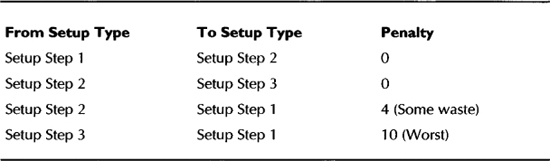
TABLE 7-5. An Example of Resource Sequence Relationships
Line Performance
When a line is laid out, the line performance must be at an acceptable level to justify the investment. Even after laying out a flow line, if a line doesn’t produce to demand, it’s only as good as a highly efficient process layout. Flow lines should produce what is required of them—both on an hourly basis and over a period of time. The two important factors that gauge the health of a flow line are Line Flow Rate and Line Linearity. Line Flow Rate is used to gauge the hourly performance of a line, whereas Line Linearity is used to gauge the performance of a line over a period of time.
Line Flow Rate
Line Flow Rate is monitored by comparing the actual line output per hour against the planned output per hour. Currently there is no standard report that does this for you, but a custom report that plots the actual completions in an hour against the planned completions will be very useful and not hard to build. You can have a standard display board in each of your lines (the important ones that you want to monitor) that will display the flow rate in the form similar to the one that is shown in Figure 7-10.

FIGURE 7-10. Monitoring Line Flow Rate
Line Linearity
Comparing the planned production to the actual production at the end of the production period conceals most of the problems. For example, let’s say that your line is supposed to produce 10 widgets everyday and the actual production is 5, 6, 6, 7, 7, 13, 13, 14, 16, 13. The difference between planned and actual production on each of these days is -5, -4, -4, -3, -3, 3, 3, 4, 6, 3, which represents the deviation from plan. At the end of the 10-day period, if you measure the total deviation by summing up these deviations, you will get a value of 0. This might appear to indicate that the line performed quite well during the period, when in reality you did not produce the correct number of widgets on any day. The process is out of control, yet the simple comparison of total planned to actual masks this fact.
Using a measure such as the Line Linearity Index will help uncover such problems. The Line Linearity Index considers the absolute deviations. The formula for line linearity is shown here:
![]()
In the previous example, the sum of all the absolute deviations is 38 and the total planned production is 100. The Line Linearity Index for your line is therefore 62 percent for the period. The goal is to improve the Line Linearity Index by minimizing the deviations from the planned production rate.
The Flow Workstation has a tab called Linearity and enables you to monitor the trend online. You can also create a visual control chart such as the one that is shown in Figure 7-11 that tracks the actual linearity against the target linearity, with a lower limit that prompts for management actions.

FIGURE 7-11. Visual control chart to monitor linearity trend with management action limit
You can use the Flow Line Linearity report that is available in the Productivity Reports window to plot these values in the visual control chart. The report shows the planned production rate, actual production rate, variance, and linearity index for the selected lines.
Summary
This chapter has discussed the types of layout supported by Oracle Applications and the suitability of these layouts to various business needs. Takt time, Operation Times, and the TPCT were discussed in detail.
The Graphical Line Designer enables you to define your routings using an easy-to-use graphical user interface that supports drag and drop of operations. The information in the Graphical Line Designer is presented in two panes—the tree hierarchy pane and the graphical network pane. You can drag and drop events between operations or processes in the graphical network pane.
The MMM enables you to identify the imbalance problems in the line. You have to iterate your line design using the Graphical Line Designer and the MMM to get an optimized layout of the line. Even after you have repeated iterations, you might not achieve a completely balanced line. In this case, you will have to use the various engineering techniques to achieve line balance or choose to carry in process kanban as a cushion.
When you have defined a completely balanced line, you can optionally generate operational method sheets using drawing software that demonstrates each event and operation to the operator. These can be attached to the event or operation, which will then serve as a reference for the operator.
Build quality into the process by including standard events such as pre-operation inspection, so that you don’t allow defective products to go through the remaining operations in the line. You can also use pre-control charts to establish online quality.
Setup types enable you to optimize your setup sequences, which will be used by Manufacturing Scheduling. This will enable you to achieve high levels of utilization for your setup resources.
Finally, anything that goes unmeasured doesn’t get improved. Use the line flow rate and line linearity to monitor your lines performance on a day-to-day basis so that you can maintain the performance of your line at an acceptable standard.