8
Index Alignment
Introduction
When Series or DataFrames are combined, each dimension of the data automatically aligns on each axis first before any computation happens. This silent and automatic alignment of axes can confuse the uninitiated, but it gives flexibility to the power user. This chapter explores the Index object in-depth before showcasing a variety of recipes that take advantage of its automatic alignment.
Examining the Index object
As was discussed previously, each axis of a Series and a DataFrame has an Index object that labels the values. There are many different types of Index objects, but they all share common behavior. All Index objects, except for the MultiIndex, are single-dimensional data structures that combine the functionality of Python sets and NumPy ndarrays.
In this recipe, we will examine the column index of the college dataset and explore much of its functionality.
How to do it…
- Read in the college dataset, and create a variable
columnsthat holds the column index:>>> import pandas as pd >>> import numpy as np >>> college = pd.read_csv("data/college.csv") >>> columns = college.columns >>> columns Index(['INSTNM', 'CITY', 'STABBR', 'HBCU', 'MENONLY', 'WOMENONLY', 'RELAFFIL', 'SATVRMID', 'SATMTMID', 'DISTANCEONLY', 'UGDS', 'UGDS_WHITE', 'UGDS_BLACK', 'UGDS_HISP', 'UGDS_ASIAN', 'UGDS_AIAN', 'UGDS_NHPI', 'UGDS_2MOR', 'UGDS_NRA', 'UGDS_UNKN', 'PPTUG_EF', 'CURROPER', 'PCTPELL', 'PCTFLOAN', 'UG25ABV', 'MD_EARN_WNE_P10', 'GRAD_DEBT_MDN_SUPP'], dtype='object') - Use the
.valuesattribute to access the underlying NumPy array:>>> columns.values array(['INSTNM', 'CITY', 'STABBR', 'HBCU', 'MENONLY', 'WOMENONLY', 'RELAFFIL', 'SATVRMID', 'SATMTMID', 'DISTANCEONLY', 'UGDS', 'UGDS_WHITE', 'UGDS_BLACK', 'UGDS_HISP', 'UGDS_ASIAN', 'UGDS_AIAN', 'UGDS_NHPI', 'UGDS_2MOR', 'UGDS_NRA', 'UGDS_UNKN', 'PPTUG_EF', 'CURROPER', 'PCTPELL', 'PCTFLOAN', 'UG25ABV', 'MD_EARN_WNE_P10', 'GRAD_DEBT_MDN_SUPP'], dtype=object) - Select items from the index by position with a scalar, list, or slice:
>>> columns[5] 'WOMENONLY' >>> columns[[1, 8, 10]] Index(['CITY', 'SATMTMID', 'UGDS'], dtype='object') >>> columns[-7:-4] Index(['PPTUG_EF', 'CURROPER', 'PCTPELL'], dtype='object') - Indexes share many of the same methods as Series and DataFrames:
>>> columns.min(), columns.max(), columns.isnull().sum() ('CITY', 'WOMENONLY', 0) - You can use basic arithmetic and comparison operators on Index objects:
>>> columns + "_A" Index(['INSTNM_A', 'CITY_A', 'STABBR_A', 'HBCU_A', 'MENONLY_A', 'WOMENONLY_A', 'RELAFFIL_A', 'SATVRMID_A', 'SATMTMID_A', 'DISTANCEONLY_A', 'UGDS_A', 'UGDS_WHITE_A', 'UGDS_BLACK_A', 'UGDS_HISP_A', 'UGDS_ASIAN_A', 'UGDS_AIAN_A', 'UGDS_NHPI_A', 'UGDS_2MOR_A', 'UGDS_NRA_A', 'UGDS_UNKN_A', 'PPTUG_EF_A', 'CURROPER_A', 'PCTPELL_A', 'PCTFLOAN_A', 'UG25ABV_A', 'MD_EARN_WNE_P10_A', 'GRAD_DEBT_MDN_SUPP_A'], dtype='object') >>> columns > "G" array([ True, False, True, True, True, True, True, True, True, False, True, True, True, True, True, True, True, True, True, True, True, False, True, True, True, True, True]) - Trying to change an Index value after its creation fails. Indexes are immutable objects:
>>> columns[1] = "city"
Traceback (most recent call last):
  ...
TypeError: Index does not support mutable operations
How it works…
As you can see from many of the Index object operations, it appears to have quite a bit in common with both Series and ndarrays. One of the most significant differences comes in step 6. Indexes are immutable and their values cannot be changed once created.
There's more…
Indexes support the set operations—union, intersection, difference, and symmetric difference:
>>> c1 = columns[:4]
>>> c1
Index(['INSTNM', 'CITY', 'STABBR', 'HBCU'], dtype='object')
>>> c2 = columns[2:6]
>>> c2
Index(['STABBR', 'HBCU', 'MENONLY', 'WOMENONLY'], dtype='object')
>>> c1.union(c2)  # or 'c1 | c2'
Index(['CITY', 'HBCU', 'INSTNM', 'MENONLY', 'STABBR', 'WOMENONLY'],
dtype='object')
>>> c1.symmetric_difference(c2)  # or 'c1 ^ c2'
Index(['CITY', 'INSTNM', 'MENONLY', 'WOMENONLY'], dtype='object')
Indexes have many of the same operations as Python sets, and are similar to Python sets in another vital way. They are (usually) implemented using hash tables, which make for extremely fast access when selecting rows or columns from a DataFrame. Because the values need to be hashable, the values for the Index object need to be immutable types, such as a string, integer, or tuple, just like the keys in a Python dictionary.
Indexes support duplicate values, and if there happens to be a duplicate in any Index, then a hash table can no longer be used for its implementation, and object access becomes much slower.
Producing Cartesian products
Whenever a Series or DataFrame operates with another Series or DataFrame, the indexes (both the row index and column index) of each object align first before any operation begins. This index alignment happens behind the scenes and can be very surprising for those new to pandas. This alignment always creates a Cartesian product between the indexes unless the indexes are identical.
A Cartesian product is a mathematical term that usually appears in set theory. A Cartesian product between two sets is all the combinations of pairs of both sets. For example, the 52 cards in a standard playing card deck represent a Cartesian product between the 13 ranks (A, 2, 3,…, Q, K) and the four suits.
Producing a Cartesian product isn't always the intended outcome, but it's essential to be aware of how and when it occurs so as to avoid unintended consequences. In this recipe, two Series with overlapping but non-identical indexes are added together, yielding a surprising result. We will also show what happens if they have the same index.
How to do it…
Follow these steps to create a Cartesian product:
- Construct two Series that have indexes that are different but contain some of the same values:
>>> s1 = pd.Series(index=list("aaab"), data=np.arange(4))
>>> s1
a    0
a    1
a    2
b    3
dtype: int64
>>> s2 = pd.Series(index=list("cababb"), data=np.arange(6))
>>> s2
c    0
a    1
b    2
a    3
b    4
b    5
dtype: int64
- Add the two Series together to produce a Cartesian product. For each
aindex value ins1,we add everyains2:>>> s1 + s2 a 1.0 a 3.0 a 2.0 a 4.0 a 3.0 a 5.0 b 5.0 b 7.0 b 8.0 c NaN dtype: float64
How it works…
Each a label in s1 pairs up with each a label in s2. This pairing produces six a labels, three b labels, and one c label in the resulting Series. A Cartesian product happens between all identical index labels.
As the element with label c is unique to the Series s2, pandas defaults its value to missing, as there is no label for it to align to in s1. pandas defaults to a missing value whenever an index label is unique to one object. This has the unfortunate consequence of changing the data type of the Series to a float, whereas each Series had only integers as values. The type change occurred because NumPy's missing value object, np.nan, only exists for floats but not for integers. Series and DataFrame columns must have homogeneous numeric data types. Therefore, each value in the column was converted to a float. Changing types makes little difference for this small dataset, but for larger datasets, this can have a significant memory impact.
There's more…
The Cartesian product is not created when the indexes are unique or contain both the same exact elements and elements in the same order. When the index values are unique or they are the same and have the same order, a Cartesian product is not created, and the indexes instead align by their position. Notice here that each element aligned exactly by position and that the data type remained an integer:
>>> s1 = pd.Series(index=list("aaabb"), data=np.arange(5))
>>> s2 = pd.Series(index=list("aaabb"), data=np.arange(5))
>>> s1 + s2
a    0
a    2
a    4
b    6
b    8
dtype: int64
If the elements of the index are identical, but the order is different between the Series, the Cartesian product occurs. Let's change the order of the index in s2 and rerun the same operation:
>>> s1 = pd.Series(index=list("aaabb"), data=np.arange(5))
>>> s2 = pd.Series(index=list("bbaaa"), data=np.arange(5))
>>> s1 + s2
a    2
a    3
a    4
a    3
a    4
    ..
a    6
b    3
b    4
b    4
b    5
Length: 13, dtype: int64
Be aware of this as pandas has two drastically different outcomes for this same operation. Another instance where this can happen is during a groupby operation. If you do a groupby with multiple columns and one is of the type categorical, you will get a Cartesian product where each outer index will have every inner index value.
Finally, we will add two Series that have index values in a different order but do not have duplicate values. When we add these, we do not get a Cartesian product:
>>> s3 = pd.Series(index=list("ab"), data=np.arange(2))
>>> s4 = pd.Series(index=list("ba"), data=np.arange(2))
>>> s3 + s4
a    1
b    1
dtype: int64
In this recipe, each Series had a different number of elements. Typically, array-like data structures in Python and other languages do not allow operations to take place when the operating dimensions do not contain the same number of elements. pandas allows this to happen by aligning the indexes first before completing the operation.
In the previous chapter, I showed that you can set a column to the index and then filter on them. My preference is to leave the index alone and filter on the columns. This section gives another example of when you need to be very careful with the index.
Exploding indexes
The previous recipe walked through a trivial example of two small Series being added together with unequal indexes. This recipe is more of an "anti-recipe" of what not to do. The Cartesian product of index alignment can produce comically incorrect results when dealing with larger amounts of data.
In this recipe, we add two larger Series that have indexes with only a few unique values but in different orders. The result will explode the number of values in the indexes.
How to do it…
- Read in the employee data and set the index to the
RACEcolumn:>>> employee = pd.read_csv( ... "data/employee.csv", index_col="RACE" ... ) >>> employee.head() UNIQUE_ID POSITION_TITLE ... HIRE_DATE JOB_DATE RACE ... Hispanic/... 0 ASSISTAN... ... 2006-06-12 2012-10-13 Hispanic/... 1 LIBRARY ... ... 2000-07-19 2010-09-18 White 2 POLICE O... ... 2015-02-03 2015-02-03 White 3 ENGINEER... ... 1982-02-08 1991-05-25 White 4 ELECTRICIAN ... 1989-06-19 1994-10-22 - Select the
BASE_SALARYcolumn as two different Series. Check to see whether this operation created two new objects:>>> salary1 = employee["BASE_SALARY"] >>> salary2 = employee["BASE_SALARY"] >>> salary1 is salary2 True - The
salary1andsalary2variables are referring to the same object. This means that any change to one will change the other. To ensure that you receive a brand new copy of the data, use the.copymethod:>>> salary2 = employee["BASE_SALARY"].copy() >>> salary1 is salary2 False - Let's change the order of the index for one of the Series by sorting it:
>>> salary1 = salary1.sort_index() >>> salary1.head() RACE American Indian or Alaskan Native 78355.0 American Indian or Alaskan Native 26125.0 American Indian or Alaskan Native 98536.0 American Indian or Alaskan Native NaN American Indian or Alaskan Native 55461.0 Name: BASE_SALARY, dtype: float64 >>> salary2.head() RACE Hispanic/Latino 121862.0 Hispanic/Latino 26125.0 White 45279.0 White 63166.0 White 56347.0 Name: BASE_SALARY, dtype: float64 - Let's add these salary Series together:
>>> salary_add = salary1 + salary2 >>> salary_add.head() RACE American Indian or Alaskan Native 138702.0 American Indian or Alaskan Native 156710.0 American Indian or Alaskan Native 176891.0 American Indian or Alaskan Native 159594.0 American Indian or Alaskan Native 127734.0 Name: BASE_SALARY, dtype: float64 - The operation completed successfully. Let's create one more Series of
salary1added to itself and then output the lengths of each Series. We just exploded the index from 2,000 values to more than one million:>>> salary_add1 = salary1 + salary1 >>> len(salary1), len(salary2), len(salary_add), len( ... salary_add1 ... ) (2000, 2000, 1175424, 2000)
How it works…
Step 2 appears at first to create two unique objects, but in fact, it creates a single object that is referred to by two different variable names. The expression employee['BASE_SALARY'], technically creates a view, and not a brand new copy. This is verified with the is operator.
In pandas, a view is not a new object but just a reference to another object, usually some subset of a DataFrame. This shared object can be a cause for many issues.
To ensure that the variables reference completely different objects, we use the .copy method and then verify that they are different objects with the is operator. Step 4 uses the .sort_index method to sort the Series by race. Note that this Series has the same index entries, but they are now in a different order than salary1. Step 5 adds these different Series together to produce the sum. By inspecting the head, it is still not clear what has been produced.
Step 6 adds salary1 to itself to show a comparison between the two different Series additions. The lengths of all the Series in this recipe are printed and we clearly see that salary_add has now exploded to over one million values. A Cartesian product took place because the indexes were not unique and in the same order. This recipe shows a more dramatic example of what happens when the indexes differ.
There's more…
We can verify the number of values of salary_add by doing a little mathematics. As a Cartesian product takes place between all of the same index values, we can sum the square of their counts. Even missing values in the index produce Cartesian products with themselves:
>>> index_vc = salary1.index.value_counts(dropna=False)
>>> index_vc
Black or African American            700
White                                665
Hispanic/Latino                      480
Asian/Pacific Islander               107
NaN                                   35
American Indian or Alaskan Native     11
Others                                 2
Name: RACE, dtype: int64
>>> index_vc.pow(2).sum()
1175424
Filling values with unequal indexes
When two Series are added together using the plus operator and one of the index labels does not appear in the other, the resulting value is always missing. pandas has the .add method, which provides an option to fill the missing value. Note that these Series do not include duplicate entries, hence there is no need to worry about a Cartesian product exploding the number of entries.
In this recipe, we add together multiple Series from the baseball dataset with unequal (but unique) indexes using the .add method with the fill_value parameter to ensure that there are no missing values in the result.
How to do it…
- Read in the three baseball datasets and set
playerIDas the index:>>> baseball_14 = pd.read_csv( ... "data/baseball14.csv", index_col="playerID" ... ) >>> baseball_15 = pd.read_csv( ... "data/baseball15.csv", index_col="playerID" ... ) >>> baseball_16 = pd.read_csv( ... "data/baseball16.csv", index_col="playerID" ... ) >>> baseball_14.head() yearID stint teamID lgID ... HBP SH SF GIDP playerID ... altuvjo01 2014 1 HOU AL ... 5.0 1.0 5.0 20.0 cartech02 2014 1 HOU AL ... 5.0 0.0 4.0 12.0 castrja01 2014 1 HOU AL ... 9.0 1.0 3.0 11.0 corpoca01 2014 1 HOU AL ... 3.0 1.0 2.0 3.0 dominma01 2014 1 HOU AL ... 5.0 2.0 7.0 23.0 - Use the
.differencemethod on the index to discover which index labels are inbaseball_14and not inbaseball_15, and vice versa:>>> baseball_14.index.difference(baseball_15.index) Index(['corpoca01', 'dominma01', 'fowlede01', 'grossro01', 'guzmaje01', 'hoeslj01', 'krausma01', 'preslal01', 'singljo02'], dtype='object', name='playerID') >>> baseball_15.index.difference(baseball_14.index) Index(['congeha01', 'correca01', 'gattiev01', 'gomezca01', 'lowrije01', 'rasmuco01', 'tuckepr01', 'valbulu01'], dtype='object', name='playerID') - There are quite a few players unique to each index. Let's find out how many hits each player has in total over the three-year period. The
Hcolumn contains the number of hits:>>> hits_14 = baseball_14["H"] >>> hits_15 = baseball_15["H"] >>> hits_16 = baseball_16["H"] >>> hits_14.head() playerID altuvjo01 225 cartech02 115 castrja01 103 corpoca01 40 dominma01 121 Name: H, dtype: int64 - Let's first add together two Series using the plus operator:
>>> (hits_14 + hits_15).head() playerID altuvjo01 425.0 cartech02 193.0 castrja01 174.0 congeha01 NaN corpoca01 NaN Name: H, dtype: float64 - Even though players
congeha01andcorpoca01have values for 2015, their result is missing. Let's use the.addmethod with thefill_valueparameter to avoid missing values:>>> hits_14.add(hits_15, fill_value=0).head() playerID altuvjo01 425.0 cartech02 193.0 castrja01 174.0 congeha01 46.0 corpoca01 40.0 Name: H, dtype: float64 - We add hits from 2016 by chaining the
addmethod once more:>>> hits_total = hits_14.add(hits_15, fill_value=0).add( ... hits_16, fill_value=0 ... ) >>> hits_total.head() playerID altuvjo01 641.0 bregmal01 53.0 cartech02 193.0 castrja01 243.0 congeha01 46.0 Name: H, dtype: float64 - Check for missing values in the result:
>>> hits_total.hasnans
False
How it works…
The .add method works in a similar way to the plus operator, but allows for more flexibility by providing the fill_value parameter to take the place of a non-matching index. In this problem, it makes sense to default the non-matching index value to 0, but you could have used any other number.
There will be occasions when each Series contains index labels that correspond to missing values. In this specific instance, when the two Series are added, the index label will still correspond to a missing value regardless of whether the fill_value parameter is used. To clarify this, take a look at the following example where the index label a corresponds to a missing value in each Series:
>>> s = pd.Series(
...     index=["a", "b", "c", "d"],
...     data=[np.nan, 3, np.nan, 1],
... )
>>> s
a    NaN
b    3.0
c    NaN
d    1.0
dtype: float64
>>> s1 = pd.Series(
...     index=["a", "b", "c"], data=[np.nan, 6, 10]
... )
>>> s1
a     NaN
b     6.0
c    10.0
dtype: float64
>>> s.add(s1, fill_value=5)
a     NaN
b     9.0
c    15.0
d     6.0
dtype: float64
There's more…
This recipe shows how to add Series with only a single index together. It is also possible to add DataFrames together. Adding two DataFrames together will align both the index and columns before computation and insert missing values for non-matching indexes. Let's start by selecting a few of the columns from the 2014 baseball dataset:
>>> df_14 = baseball_14[["G", "AB", "R", "H"]]
>>> df_14.head()
             G   AB   R    H
playerID
altuvjo01  158  660  85  225
cartech02  145  507  68  115
castrja01  126  465  43  103
corpoca01   55  170  22   40
dominma01  157  564  51  121
Let's also select a few of the same and a few different columns from the 2015 baseball dataset:
>>> df_15 = baseball_15[["AB", "R", "H", "HR"]]
>>> df_15.head()
            AB   R    H  HR
playerID
altuvjo01  638  86  200  15
cartech02  391  50   78  24
castrja01  337  38   71  11
congeha01  201  25   46  11
correca01  387  52  108  22
Adding the two DataFrames together creates missing values wherever rows or column labels cannot align. You can use the .style attribute and call the .highlight_null method to see where the missing values are:

Highlight null values when using the plus operator
Only the rows where playerID appears in both DataFrames will be available. Similarly, the columns AB, H, and R are the only ones that appear in both DataFrames. Even if we use the .add method with the fill_value parameter specified, we still might have missing values. This is because some combinations of rows and columns never existed in our input data; for example, the intersection of playerID congeha01 and column G. That player only appeared in the 2015 dataset that did not have the G column. Therefore, that value was missing:
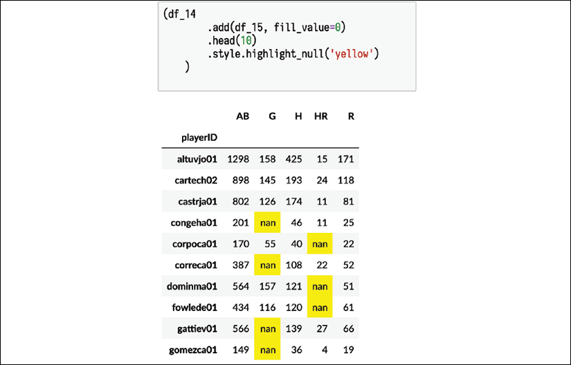
Highlight null values when using the .add method
Adding columns from different DataFrames
All DataFrames can add new columns to themselves. However, as usual, whenever a DataFrame is adding a new column from another DataFrame or Series, the indexes align first, and then the new column is created.
This recipe uses the employee dataset to append a new column containing the maximum salary of that employee's department.
How to do it…
- Import the employee data and select the
DEPARTMENTandBASE_SALARYcolumns in a new DataFrame:>>> employee = pd.read_csv("data/employee.csv") >>> dept_sal = employee[["DEPARTMENT", "BASE_SALARY"]] - Sort this smaller DataFrame by salary within each department:
>>> dept_sal = dept_sal.sort_values( ... ["DEPARTMENT", "BASE_SALARY"], ... ascending=[True, False], ... ) - Use the
.drop_duplicatesmethod to keep the first row of eachDEPARTMENT:>>> max_dept_sal = dept_sal.drop_duplicates( ... subset="DEPARTMENT" ... ) >>> max_dept_sal.head() DEPARTMENT BASE_SALARY DEPARTMENT BASE_SALARY 1494 Admn. & Regulatory Affairs 140416.0 149 City Controller's Office 64251.0 236 City Council 100000.0 647 Convention and Entertainment 38397.0 1500 Dept of Neighborhoods (DON) 89221.0 - Put the
DEPARTMENTcolumn into the index for each DataFrame:>>> max_dept_sal = max_dept_sal.set_index("DEPARTMENT") >>> employee = employee.set_index("DEPARTMENT") - Now that the indexes contain matching values, we can add a new column to the employee DataFrame:
>>> employee = employee.assign( ... MAX_DEPT_SALARY=max_dept_sal["BASE_SALARY"] ... ) >>> employee UNIQUE_ID ... MAX_D/ALARY DEPARTMENT ... Municipal Courts Department 0 ... 121862.0 Library 1 ... 107763.0 Houston Police Department-HPD 2 ... 199596.0 Houston Fire Department (HFD) 3 ... 210588.0 General Services Department 4 ... 89194.0 ... ... ... ... Houston Police Department-HPD 1995 ... 199596.0 Houston Fire Department (HFD) 1996 ... 210588.0 Houston Police Department-HPD 1997 ... 199596.0 Houston Police Department-HPD 1998 ... 199596.0 Houston Fire Department (HFD) 1999 ... 210588.0 - We can validate our results with the query method to check whether there exist any rows where
BASE_SALARYis greater thanMAX_DEPT_SALARY:>>> employee.query("BASE_SALARY > MAX_DEPT_SALARY") Empty DataFrame Columns: [UNIQUE_ID, POSITION_TITLE, BASE_SALARY, RACE, EMPLOYMENT_TYPE, GENDER, EMPLOYMENT_STATUS, HIRE_DATE, JOB_DATE, MAX_DEPT_SALARY] Index: [] - Refactor our code into a chain:
>>> employee = pd.read_csv("data/employee.csv")
>>> max_dept_sal = (
...     employee
...     [["DEPARTMENT", "BASE_SALARY"]]
...     .sort_values(
...         ["DEPARTMENT", "BASE_SALARY"],
...         ascending=[True, False],
...     )
...     .drop_duplicates(subset="DEPARTMENT")
...     .set_index("DEPARTMENT")
... )
>>> (
...     employee
...     .set_index("DEPARTMENT")
...     .assign(
...         MAX_DEPT_SALARY=max_dept_sal["BASE_SALARY"]
...     )
... )
              UNIQUE_ID POSITION_TITLE  ...    JOB_DATE MAX_DEPT_SALARY
DEPARTMENT                              ...
Municipal...          0  ASSISTAN...    ...  2012-10-13     121862.0
Library               1  LIBRARY ...    ...  2010-09-18     107763.0
Houston P...          2  POLICE O...    ...  2015-02-03     199596.0
Houston F...          3  ENGINEER...    ...  1991-05-25     210588.0
General S...          4  ELECTRICIAN    ...  1994-10-22      89194.0
...                 ...          ...    ...         ...          ...
Houston P...       1995  POLICE O...    ...  2015-06-09     199596.0
Houston F...       1996  COMMUNIC...    ...  2013-10-06     210588.0
Houston P...       1997  POLICE O...    ...  2015-10-13     199596.0
Houston P...       1998  POLICE O...    ...  2011-07-02     199596.0
Houston F...       1999  FIRE FIG...    ...  2010-07-12     210588.0
How it works…
Steps 2 and 3 find the maximum salary for each department. For automatic index alignment to work properly, we set each DataFrame index as the department. Step 5 works because each row index from the left DataFrame, employee, aligns with one, and only one, index from the right DataFrame, max_dept_sal. If max_dept_sal has duplicates of any departments in its index, then we will get a Cartesian product.
For instance, let's see what happens when we use a DataFrame on the right-hand side of the equality that has repeated index values. We use the .sample DataFrame method to randomly choose 10 rows without replacement:
>>> random_salary = dept_sal.sample(
...     n=10, random_state=42
... ).set_index("DEPARTMENT")
>>> random_salary
                                BASE_SALARY
DEPARTMENT
Public Works & Engineering-PWE      34861.0
Houston Airport System (HAS)        29286.0
Houston Police Department-HPD       31907.0
Houston Police Department-HPD       66614.0
Houston Police Department-HPD       42000.0
Houston Police Department-HPD       43443.0
Houston Police Department-HPD       66614.0
Public Works & Engineering-PWE      52582.0
Finance                             93168.0
Houston Police Department-HPD       35318.0
Notice how there are several repeated departments in the index. When we attempt to create a new column, an error is raised alerting us that there are duplicates. At least one index label in the employee DataFrame is joining with two or more index labels from random_salary:
>>> employee["RANDOM_SALARY"] = random_salary["BASE_SALARY"]
Traceback (most recent call last):
...
ValueError: cannot reindex from a duplicate axis
There's more…
During alignment, if there is nothing for the DataFrame index to align to, the resulting value will be missing. Let's create an example where this happens. We will use only the first three rows of the max_dept_sal Series to create a new column:
>>> (
...     employee
...     .set_index("DEPARTMENT")
...     .assign(
...         MAX_SALARY2=max_dept_sal["BASE_SALARY"].head(3)
...     )
...     .MAX_SALARY2
...     .value_counts(dropna=False)
... )
NaN         1955
140416.0      29
100000.0      11
64251.0        5
Name: MAX_SALARY2, dtype: int64
The operation completed successfully but filled in salaries for only three of the departments. All the other departments that did not appear in the first three rows of the max_dept_sal Series resulted in a missing value.
My preference is to use the following code rather than the code in step 7. This code uses the .groupby method combined with the .transform method, which is discussed in a later chapter. This code reads much cleaner to me. It is shorter and does not mess with reassigning the index:
>>> max_sal = (
...     employee
...     .groupby("DEPARTMENT")
...     .BASE_SALARY
...     .transform("max")
... )
>>> (employee.assign(MAX_DEPT_SALARY=max_sal))
UNIQUE_ID POSITION_TITLE  ...    JOB_DATE  MAX_DEPT_SALARY
0             0  ASSISTAN...    ...  2012-10-13     121862.0
1             1  LIBRARY ...    ...  2010-09-18     107763.0
2             2  POLICE O...    ...  2015-02-03     199596.0
3             3  ENGINEER...    ...  1991-05-25     210588.0
4             4  ELECTRICIAN    ...  1994-10-22      89194.0
...         ...          ...    ...         ...          ...
1995       1995  POLICE O...    ...  2015-06-09     199596.0
1996       1996  COMMUNIC...    ...  2013-10-06     210588.0
1997       1997  POLICE O...    ...  2015-10-13     199596.0
1998       1998  POLICE O...    ...  2011-07-02     199596.0
1999       1999  FIRE FIG...    ...  2010-07-12     210588.0
This works because .transform preserves the original index. If you did a .groupby that creates a new index, you can use the .merge method to combine the data. We just need to tell it to merge on DEPARTMENT for the left side and the index for the right side:
>>> max_sal = (
...     employee
...     .groupby("DEPARTMENT")
...     .BASE_SALARY
...     .max()
... )
>>> (
...     employee.merge(
...         max_sal.rename("MAX_DEPT_SALARY"),
...         how="left",
...         left_on="DEPARTMENT",
...         right_index=True,
...     )
... )
UNIQUE_ID POSITION_TITLE  ...    JOB_DATE  MAX_DEPT_SALARY
0             0  ASSISTAN...    ...  2012-10-13     121862.0
1             1  LIBRARY ...    ...  2010-09-18     107763.0
2             2  POLICE O...    ...  2015-02-03     199596.0
3             3  ENGINEER...    ...  1991-05-25     210588.0
4             4  ELECTRICIAN    ...  1994-10-22      89194.0
...         ...          ...    ...         ...          ...
1995       1995  POLICE O...    ...  2015-06-09     199596.0
1996       1996  COMMUNIC...    ...  2013-10-06     210588.0
1997       1997  POLICE O...    ...  2015-10-13     199596.0
1998       1998  POLICE O...    ...  2011-07-02     199596.0
1999       1999  FIRE FIG...    ...  2010-07-12     210588.0
Highlighting the maximum value from each column
The college dataset has many numeric columns describing different metrics about each school. Many people are interested in schools that perform the best for specific metrics.
This recipe discovers the school that has the maximum value for each numeric column and styles the DataFrame to highlight the information.
How to do it…
- Read the college dataset with the institution name as the index:
>>> college = pd.read_csv( ... "data/college.csv", index_col="INSTNM" ... ) >>> college.dtypes CITY object STABBR object HBCU float64 MENONLY float64 WOMENONLY float64 ... PCTPELL float64 PCTFLOAN float64 UG25ABV float64 MD_EARN_WNE_P10 object GRAD_DEBT_MDN_SUPP object Length: 26, dtype: object - All the other columns besides
CITYandSTABBRappear to be numeric. Examining the data types from the preceding step reveals unexpectedly that theMD_EARN_WNE_P10andGRAD_DEBT_MDN_SUPPcolumns are of theobjecttype and not numeric. To help get a better idea of what kinds of values are in these columns, let's examine a sample from them:>>> college.MD_EARN_WNE_P10.sample(10, random_state=42) INSTNM Career Point College 20700 Ner Israel Rabbinical College PrivacyS... Reflections Academy of Beauty NaN Capital Area Technical College 26400 West Virginia University Institute of Technology 43400 Mid-State Technical College 32000 Strayer University-Huntsville Campus 49200 National Aviation Academy of Tampa Bay 45000 University of California-Santa Cruz 43000 Lexington Theological Seminary NaN Name: MD_EARN_WNE_P10, dtype: object >>> college.GRAD_DEBT_MDN_SUPP.sample(10, random_state=42) INSTNM Career Point College 14977 Ner Israel Rabbinical College PrivacyS... Reflections Academy of Beauty PrivacyS... Capital Area Technical College PrivacyS... West Virginia University Institute of Technology 23969 Mid-State Technical College 8025 Strayer University-Huntsville Campus 36173.5 National Aviation Academy of Tampa Bay 22778 University of California-Santa Cruz 19884 Lexington Theological Seminary PrivacyS... Name: GRAD_DEBT_MDN_SUPP, dtype: object - These values are strings, but we would like them to be numeric. I like to use the
.value_countsmethod in this case to see whether it reveals any characters that forced the column to be non-numeric:>>> college.MD_EARN_WNE_P10.value_counts() PrivacySuppressed 822 38800 151 21500 97 49200 78 27400 46 ... 66700 1 163900 1 64400 1 58700 1 64100 1 Name: MD_EARN_WNE_P10, Length: 598, dtype: int64 >>> set(college.MD_EARN_WNE_P10.apply(type)) {<class 'float'>, <class 'str'>} >>> college.GRAD_DEBT_MDN_SUPP.value_counts() PrivacySuppressed 1510 9500 514 27000 306 25827.5 136 25000 124 ... 16078.5 1 27763.5 1 6382 1 27625 1 11300 1 Name: GRAD_DEBT_MDN_SUPP, Length: 2038, dtype: int64 - The culprit appears to be that some schools have privacy concerns about these two columns of data. To force these columns to be numeric, use the pandas function
to_numeric. If we use theerrors='coerce'parameter, it will convert those values toNaN:>>> cols = ["MD_EARN_WNE_P10", "GRAD_DEBT_MDN_SUPP"] >>> for col in cols: ... college[col] = pd.to_numeric( ... college[col], errors="coerce" ... ) >>> college.dtypes.loc[cols] MD_EARN_WNE_P10 float64 GRAD_DEBT_MDN_SUPP float64 dtype: object - Use the
.select_dtypesmethod to filter for only numeric columns. This will excludeSTABBRandCITYcolumns, where a maximum value doesn't make sense with this problem:>>> college_n = college.select_dtypes("number") >>> college_n.head() HBCU MENONLY ... MD_EARN_WNE_P10 GRAD_DEBT_MDN_SUPP INSTNM ... Alabama A... 1.0 0.0 ... 30300.0 33888.0 Universit... 0.0 0.0 ... 39700.0 21941.5 Amridge U... 0.0 0.0 ... 40100.0 23370.0 Universit... 0.0 0.0 ... 45500.0 24097.0 Alabama S... 1.0 0.0 ... 26600.0 33118.5 - Several columns have binary only (0 or 1) values that will not provide useful information for maximum values. To find these columns, we can create a Boolean Series and find all the columns that have two unique values with the
.nuniquemethod:>>> binary_only = college_n.nunique() == 2 >>> binary_only.head() HBCU True MENONLY True WOMENONLY True RELAFFIL True SATVRMID False dtype: bool - Use the Boolean array to create a list of binary columns:
>>> binary_cols = binary_only[binary_only].index >>> binary_cols Index(['HBCU', 'MENONLY', 'WOMENONLY', 'RELAFFIL', 'DISTANCEONLY', 'CURROPER'], dtype='object') - Since we are looking for the maximum values, we can drop the binary columns using the
.dropmethod:>>> college_n2 = college_n.drop(columns=binary_cols) >>> college_n2.head() SATVRMID SATMTMID ... MD_EARN_WNE_P10 GRAD_DEBT_MDN_SUPP INSTNM ... Alabama A... 424.0 420.0 ... 30300.0 33888.0 Universit... 570.0 565.0 ... 39700.0 21941.5 Amridge U... NaN NaN ... 40100.0 23370.0 Universit... 595.0 590.0 ... 45500.0 24097.0 Alabama S... 425.0 430.0 ... 26600.0 33118.5 - Now we can use the
.idxmaxmethod to find the index label of the maximum value for each column:>>> max_cols = college_n2.idxmax() >>> max_cols SATVRMID California Institute of Technology SATMTMID California Institute of Technology UGDS University of Phoenix-Arizona UGDS_WHITE Mr Leon's School of Hair Design-Moscow UGDS_BLACK Velvatex College of Beauty Culture ... PCTPELL MTI Business College Inc PCTFLOAN ABC Beauty College Inc UG25ABV Dongguk University-Los Angeles MD_EARN_WNE_P10 Medical College of Wisconsin GRAD_DEBT_MDN_SUPP Southwest University of Visual Arts-Tucson Length: 18, dtype: object - Call the
.uniquemethod on themax_colsSeries. This returns an ndarray of the index values incollege_n2that has the maximum values:>>> unique_max_cols = max_cols.unique() >>> unique_max_cols[:5] array(['California Institute of Technology', 'University of Phoenix-Arizona', "Mr Leon's School of Hair Design-Moscow", 'Velvatex College of Beauty Culture', 'Thunderbird School of Global Management'], dtype=object) - Use the values of
max_colsto select only those rows that have schools with a maximum value and then use the.styleattribute to highlight these values:college_n2.loc[unique_max_cols].style.highlight_max()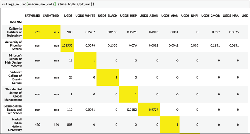
Display maximum column values
- Refactor the code to make it easier to read:
>>> def remove_binary_cols(df):
...     binary_only = df.nunique() == 2
...     cols = binary_only[binary_only].index.tolist()
...     return df.drop(columns=cols)
>>> def select_rows_with_max_cols(df):
...     max_cols = df.idxmax()
...     unique = max_cols.unique()
...     return df.loc[unique]
>>> (
...     college
...     .assign(
...         MD_EARN_WNE_P10=pd.to_numeric(
...             college.MD_EARN_WNE_P10, errors="coerce"
...         ),
...         GRAD_DEBT_MDN_SUPP=pd.to_numeric(
...             college.GRAD_DEBT_MDN_SUPP, errors="coerce"
...         ),
...     )
...     .select_dtypes("number")
...     .pipe(remove_binary_cols)
...     .pipe(select_rows_with_max_cols)
... )
              SATVRMID  SATMTMID  ...  MD_EARN_WNE_P10  GRAD_DEBT_MDN_SUPP
INSTNM                            ...
Californi...     765.0     785.0  ...      77800.0          11812.5
Universit...       NaN       NaN  ...          NaN          33000.0
Mr Leon's...       NaN       NaN  ...          NaN          15710.0
Velvatex ...       NaN       NaN  ...          NaN              NaN
Thunderbi...       NaN       NaN  ...     118900.0              NaN
...                ...       ...  ...          ...              ...
MTI Busin...       NaN       NaN  ...      23000.0           9500.0
ABC Beaut...       NaN       NaN  ...          NaN          16500.0
Dongguk U...       NaN       NaN  ...          NaN              NaN
Medical C...       NaN       NaN  ...     233100.0              NaN
Southwest...       NaN       NaN  ...      27200.0          49750.0
How it works…
The .idxmax method is a useful method, especially when the index is meaningfully labeled. It was unexpected that both MD_EARN_WNE_P10 and GRAD_DEBT_MDN_SUPP were of the object data type. When loading CSV files, pandas lists the column as an object type (even though it might contain both number and string types) if the column contains at least one string.
By examining a specific column value in step 2, we were able to discover that we had strings in these columns. In step 3, we use the .value_counts method to reveal offending characters. We uncover the PrivacySuppressed values that are causing havoc.
pandas can force all strings that contain only numeric characters to numeric data types with the to_numeric function. We do this in step 4. To override the default behavior of raising an error when to_numeric encounters a string that cannot be converted, you must pass coerce to the errors parameter. This forces all non-numeric character strings to become missing values (np.nan).
Several columns do not have useful or meaningful maximum values. They were removed in step 5 through step 8. The .select_dtypes method can be beneficial for wide DataFrames with many columns.
In step 9, .idxmax iterates through all the columns to find the index of the maximum value for each column. It outputs the results as a Series. The school with both the highest SAT math and verbal scores is California Institute of Technology, while Dongguk University Los Angeles has the highest number of students older than 25.
Although the information provided by .idxmax is convenient, it does not yield the corresponding maximum value. To do this, we gather all the unique school names from the values of the max_cols Series in step 10.
Next, in step 11, we index off a .loc to select rows based on the index label, which was set to school names when loading the CSV in the first step. This filters for only schools that have a maximum value. DataFrames have a .style attribute that itself has some methods to alter the appearance of the displayed DataFrame. Highlighting the maximum value makes the result much clearer.
Finally, we refactor the code to make it a clean pipeline.
There's more…
By default, the .highlight_max method highlights the maximum value of each column. We can use the axis parameter to highlight the maximum value of each row instead. Here, we select just the race percentage columns of the college dataset and highlight the race with the highest percentage for each school:
>>> college = pd.read_csv(
...     "data/college.csv", index_col="INSTNM"
... )
>>> college_ugds = college.filter(like="UGDS_").head()

Display maximum column values
Replicating idxmax with method chaining
A good exercise is to attempt an implementation of a built-in DataFrame method on your own. This type of replication can give you a deeper understanding of other pandas methods that you normally wouldn't have come across. .idxmax is a challenging method to replicate using only the methods covered thus far in the book.
This recipe slowly chains together basic methods to eventually find all the row index values that contain a maximum column value.
How to do it…
- Load in the college dataset and execute the same operations as the previous recipe to get only the numeric columns that are of interest:
>>> def remove_binary_cols(df): ... binary_only = df.nunique() == 2 ... cols = binary_only[binary_only].index.tolist() ... return df.drop(columns=cols) >>> college_n = ( ... college ... .assign( ... MD_EARN_WNE_P10=pd.to_numeric( ... college.MD_EARN_WNE_P10, errors="coerce" ... ), ... GRAD_DEBT_MDN_SUPP=pd.to_numeric( ... college.GRAD_DEBT_MDN_SUPP, errors="coerce" ... ), ... ) ... .select_dtypes("number") ... .pipe(remove_binary_cols) ... ) - Find the maximum of each column with the
.maxmethod:>>> college_n.max().head() SATVRMID 765.0 SATMTMID 785.0 UGDS 151558.0 UGDS_WHITE 1.0 UGDS_BLACK 1.0 dtype: float64 - Use the
.eqDataFrame method to test each value against the column.maxmethod. By default, the.eqmethod aligns the columns of the column DataFrame with the labels of the passed Series index:>>> college_n.eq(college_n.max()).head() SATVRMID SATMTMID ... MD_EARN_WNE_P10 GRAD_DEBT_MDN_SUPP INSTNM ... Alabama A... False False ... False False Universit... False False ... False False Amridge U... False False ... False False Universit... False False ... False False Alabama S... False False ... False False - All the rows in this DataFrame that have at least one
Truevalue must contain a column maximum. Let's use the.anymethod to find all such rows that have at least oneTruevalue:>>> has_row_max = ( ... college_n ... .eq(college_n.max()) ... .any(axis="columns") ... ) >>> has_row_max.head() INSTNM Alabama A & M University False University of Alabama at Birmingham False Amridge University False University of Alabama in Huntsville False Alabama State University False dtype: bool - There are only 18 columns, which means that there should only be at most 18
Truevalues inhas_row_max. Let's find out how many there are:>>> college_n.shape (7535, 18) >>> has_row_max.sum() 401 - This was a bit unexpected, but it turns out that there are columns with many rows that equal the maximum value. This is common with many of the percentage columns that have a maximum of 1.
.idxmaxreturns the first occurrence of the maximum value. Let's back up a bit, remove the.anymethod, and look at the output from step 3. Let's run the.cumsummethod instead to accumulate all theTruevalues:>>> college_n.eq(college_n.max()).cumsum() SATVRMID SATMTMID ... MD_EARN_WNE_P10 GRAD_DEBT_MDN_SUPP INSTNM ... Alabama A... 0 0 ... 0 0 Universit... 0 0 ... 0 0 Amridge U... 0 0 ... 0 0 Universit... 0 0 ... 0 0 Alabama S... 0 0 ... 0 0 ... ... ... ... ... ... SAE Insti... 1 1 ... 1 2 Rasmussen... 1 1 ... 1 2 National ... 1 1 ... 1 2 Bay Area ... 1 1 ... 1 2 Excel Lea... 1 1 ... 1 2 - Some columns have one unique maximum, like
SATVRMIDandSATMTMID, while others likeUGDS_WHITEhave many. 109 schools have 100% of their undergraduates as White. If we chain the.cumsummethod one more time, the value 1 would only appear once in each column and it would be the first occurrence of the maximum:>>> (college_n.eq(college_n.max()).cumsum().cumsum()) SATVRMID SATMTMID ... MD_EARN_WNE_P10 GRAD_DEBT_MDN_SUPP INSTNM ... Alabama A... 0 0 ... 0 0 Universit... 0 0 ... 0 0 Amridge U... 0 0 ... 0 0 Universit... 0 0 ... 0 0 Alabama S... 0 0 ... 0 0 ... ... ... ... ... ... SAE Insti... 7305 7305 ... 3445 10266 Rasmussen... 7306 7306 ... 3446 10268 National ... 7307 7307 ... 3447 10270 Bay Area ... 7308 7308 ... 3448 10272 Excel Lea... 7309 7309 ... 3449 10274 - We can now test the equality of each value against 1 with the
.eqmethod and then use the.anymethod to find rows that have at least oneTruevalue:>>> has_row_max2 = ( ... college_n.eq(college_n.max()) ... .cumsum() ... .cumsum() ... .eq(1) ... .any(axis="columns") ... ) >>> has_row_max2.head() INSTNM Alabama A & M University False University of Alabama at Birmingham False Amridge University False University of Alabama in Huntsville False Alabama State University False dtype: bool - Check that
has_row_max2has no moreTruevalues than the number of columns:>>> has_row_max2.sum() 16 - We need all the institutions where
has_row_max2isTrue. We can use Boolean indexing on the Series itself:>>> idxmax_cols = has_row_max2[has_row_max2].index >>> idxmax_cols Index(['Thunderbird School of Global Management', 'Southwest University of Visual Arts-Tucson', 'ABC Beauty College Inc', 'Velvatex College of Beauty Culture', 'California Institute of Technology', 'Le Cordon Bleu College of Culinary Arts-San Francisco', 'MTI Business College Inc', 'Dongguk University-Los Angeles', 'Mr Leon's School of Hair Design-Moscow', 'Haskell Indian Nations University', 'LIU Brentwood', 'Medical College of Wisconsin', 'Palau Community College', 'California University of Management and Sciences', 'Cosmopolitan Beauty and Tech School', 'University of Phoenix-Arizona'], dtype='object', name='INSTNM') - All 16 of these institutions are the index of the first maximum occurrence for at least one of the columns. We can check whether they are the same as the ones found with the
.idxmaxmethod:>>> set(college_n.idxmax().unique()) == set(idxmax_cols) True - Refactor to an
idx_maxfunction:>>> def idx_max(df): ... has_row_max = ( ... df ... .eq(df.max()) ... .cumsum() ... .cumsum() ... .eq(1) ... .any(axis="columns") ... ) ... return has_row_max[has_row_max].index >>> idx_max(college_n) Index(['Thunderbird School of Global Management', 'Southwest University of Visual Arts-Tucson', 'ABC Beauty College Inc', 'Velvatex College of Beauty Culture', 'California Institute of Technology', 'Le Cordon Bleu College of Culinary Arts-San Francisco', 'MTI Business College Inc', 'Dongguk University-Los Angeles', 'Mr Leon's School of Hair Design-Moscow', 'Haskell Indian Nations University', 'LIU Brentwood', 'Medical College of Wisconsin', 'Palau Community College', 'California University of Management and Sciences', 'Cosmopolitan Beauty and Tech School', 'University of Phoenix-Arizona'], dtype='object', name='INSTNM')
How it works…
The first step replicates work from the previous recipe by converting two columns to numeric and eliminating the binary columns. We find the maximum value of each column in step 2. Care needs to be taken here as pandas silently drops columns that cannot produce a maximum. If this happens, then step 3 will still complete but provide False values for each column without an available maximum.
Step 4 uses the .any method to scan across each row in search of at least one True value. Any row with at least one True value contains a maximum value for a column. We sum up the resulting Boolean Series in step 5 to determine how many rows contain a maximum. Somewhat unexpectedly, there are far more rows than columns. Step 6 gives an insight into why this happens. We take a cumulative sum of the output from step 3 and detect the total number of rows that equal the maximum for each column.
Many colleges have 100% of their student population as only a single race. This is by far the largest contributor to the multiple rows with maximums. As you can see, there is only one row with a maximum value for both SAT score columns and undergraduate population, but several of the race columns have a tie for the maximum.
Our goal is to find the first row with the maximum value. We need to take the cumulative sum once more so that each column has only a single row equal to 1. Step 8 formats the code to have one method per line and runs the .any method as was done in step 4. If this step is successful, then we should have no more True values than the number of columns. Step 9 asserts that this is true.
To validate that we have found the same columns as .idxmax in the previous columns, we use Boolean selection on has_row_max2 with itself. The columns will be in a different order, so we convert the sequence of column names to sets, which are inherently unordered to compare equality.
There's more…
It is possible to complete this recipe in one long line of code chaining the indexing operator with an anonymous function. This little trick removes the need for step 10. We can time the difference between the .idxmax method and our manual effort in this recipe:
>>> def idx_max(df):
...     has_row_max = (
...         df
...         .eq(df.max())
...         .cumsum()
...         .cumsum()
...         .eq(1)
...         .any(axis="columns")
...         [lambda df_: df_]
...         .index
...     )
...     return has_row_max
>>> %timeit college_n.idxmax().values
1.12 ms ± 28.4 μs per loop (mean ± std. dev. of 7 runs, 1000 loops each)
>>> %timeit idx_max(college_n)
5.35 ms ± 55.2 μs per loop (mean ± std. dev. of 7 runs, 100 loops each)
Our effort is, unfortunately, five times as slow as the built-in .idxmax pandas method, but regardless of its performance regression, many creative and practical solutions use the accumulation methods like .cumsum with Boolean Series to find streaks or specific patterns along an axis.
Finding the most common maximum of columns
The college dataset contains the undergraduate population percentage of eight different races for over 7,500 colleges. It would be interesting to find the race with the highest undergrad population for each school and then find the distribution of this result for the entire dataset. We would be able to answer a question like, "What percentage of institutions have more White students than any other race?"
In this recipe, we find the race with the highest percentage of the undergraduate population for each school with the .idxmax method and then find the distribution of these maximums.
How to do it…
- Read in the college dataset and select just those columns with undergraduate race percentage information:
>>> college = pd.read_csv( ... "data/college.csv", index_col="INSTNM" ... ) >>> college_ugds = college.filter(like="UGDS_") >>> college_ugds.head() UGDS_WHITE UGDS_BLACK ... UGDS_NRA UGDS_UNKN INSTNM ... Alabama A... 0.0333 0.9353 ... 0.0059 0.0138 Universit... 0.5922 0.2600 ... 0.0179 0.0100 Amridge U... 0.2990 0.4192 ... 0.0000 0.2715 Universit... 0.6988 0.1255 ... 0.0332 0.0350 Alabama S... 0.0158 0.9208 ... 0.0243 0.0137 - Use the
.idxmaxmethod applied against the column axis to get the college name with the highest race percentage for each row:>>> highest_percentage_race = college_ugds.idxmax( ... axis="columns" ... ) >>> highest_percentage_race.head() INSTNM Alabama A & M University University of Alabama at Birmingham Amridge University University of Alabama in Huntsville Alabama State University dtype: object - Use the
.value_countsmethod to return the distribution of maximum occurrences. Add thenormalize=Trueparameter so that it sums to 1:>>> highest_percentage_race.value_counts(normalize=True) UGDS_WHITE 0.670352 UGDS_BLACK 0.151586 UGDS_HISP 0.129473 UGDS_UNKN 0.023422 UGDS_ASIAN 0.012074 UGDS_AIAN 0.006110 UGDS_NRA 0.004073 UGDS_NHPI 0.001746 UGDS_2MOR 0.001164 dtype: float64
How it works…
The key to this recipe is recognizing that the columns all represent the same unit of information. We can compare these columns with each other, which is usually not the case. For instance, it wouldn't make sense to compare SAT verbal scores with the undergraduate population. As the data is structured in this manner, we can apply the .idxmax method to each row of data to find the column with the largest value. We need to alter its default behavior with the axis parameter.
Step 3 completes this operation and returns a Series, to which we can now apply the .value_counts method to return the distribution. We pass True to the normalize parameter as we are interested in the distribution (relative frequency) and not the raw counts.
There's more…
We might want to explore more and answer the question: For those schools with more Black students than any other race, what is the distribution of its second highest race percentage?
>>> (
...     college_ugds
...     [highest_percentage_race == "UGDS_BLACK"]
...     .drop(columns="UGDS_BLACK")
...     .idxmax(axis="columns")
...     .value_counts(normalize=True)
... )
UGDS_WHITE    0.661228
UGDS_HISP     0.230326
UGDS_UNKN     0.071977
UGDS_NRA      0.018234
UGDS_ASIAN    0.009597
UGDS_2MOR     0.006718
UGDS_AIAN     0.000960
UGDS_NHPI     0.000960
dtype: float64
We needed to drop the UGDS_BLACK column before applying the same method from this recipe. It seems that these schools with higher Black populations tend to have higher Hispanic populations.