
12
Time Series Analysis
Introduction
The roots of pandas lay in analyzing financial time series data. Time series are points of data gathered over time. Generally, the time is evenly spaced between each data point. However, there may be gaps in the observations. pandas includes functionality to manipulate dates, aggregate over different time periods, sample different periods of time, and more.
Understanding the difference between Python and pandas date tools
Before we get to pandas, it can help to be aware of and understand core Python's date and time functionality. The datetime module provides three data types: date, time, and datetime. Formally, a date is a moment in time consisting of just the year, month, and day. For instance, June 7, 2013 would be a date. A time consists of hours, minutes, seconds, and microseconds (one-millionth of a second) and is unattached to any date. An example of time would be 12 hours and 30 minutes. A datetime consists of both the elements of a date and time together.
On the other hand, pandas has a single object to encapsulate date and time called a Timestamp. It has nanosecond (one-billionth of a second) precision and is derived from NumPy's datetime64 data type. Both Python and pandas each have a timedelta object that is useful when doing date addition and subtraction.
In this recipe, we will first explore Python's datetime module and then turn to the corresponding date tools in pandas.
How to do it…
- Let's begin by importing the
datetimemodule into our namespace and creating adate,time, anddatetimeobject:>>> import pandas as pd >>> import numpy as np >>> import datetime >>> date = datetime.date(year=2013, month=6, day=7) >>> time = datetime.time(hour=12, minute=30, ... second=19, microsecond=463198) >>> dt = datetime.datetime(year=2013, month=6, day=7, ... hour=12, minute=30, second=19, ... microsecond=463198) >>> print(f"date is {date}") date is 2013-06-07 >>> print(f"time is {time}") time is 12:30:19.463198 >>> print(f"datetime is {dt}") datetime is 2013-06-07 12:30:19.463198 - Let's construct and print out a
timedeltaobject, the other major data type from thedatetimemodule:>>> td = datetime.timedelta(weeks=2, days=5, hours=10, ... minutes=20, seconds=6.73, ... milliseconds=99, microseconds=8) >>> td datetime.timedelta(days=19, seconds=37206, microseconds=829008) - Add this
tdto thedateanddtobjects from step 1:>>> print(f'new date is {date+td}') new date is 2013-06-26 >>> print(f'new datetime is {dt+td}') new datetime is 2013-06-26 22:50:26.292206 - Attempting to add a
timedeltato atimeobject is not possible:>>> time + td Traceback (most recent call last): ... TypeError: unsupported operand type(s) for +: 'datetime.time' and 'datetime.timedelta' - Let's turn to pandas and its
Timestampobject, which is a moment in time with nanosecond precision. TheTimestampconstructor is very flexible, and handles a wide variety of inputs:>>> pd.Timestamp(year=2012, month=12, day=21, hour=5, ... minute=10, second=8, microsecond=99) Timestamp('2012-12-21 05:10:08.000099') >>> pd.Timestamp('2016/1/10') Timestamp('2016-01-10 00:00:00') >>> pd.Timestamp('2014-5/10') Timestamp('2014-05-10 00:00:00') >>> pd.Timestamp('Jan 3, 2019 20:45.56') Timestamp('2019-01-03 20:45:33') >>> pd.Timestamp('2016-01-05T05:34:43.123456789') Timestamp('2016-01-05 05:34:43.123456789') - It's also possible to pass in a single integer or float to the
Timestampconstructor, which returns a date equivalent to the number of nanoseconds after the Unix epoch (January 1, 1970):>>> pd.Timestamp(500) Timestamp('1970-01-01 00:00:00.000000500') >>> pd.Timestamp(5000, unit='D') Timestamp('1983-09-10 00:00:00') - pandas provides the
to_datetimefunction that works similarly to theTimestampconstructor, but comes with a few different parameters for special situations. This comes in useful for converting string columns in DataFrames to dates.But it also works on scalar dates; see the following examples:
>>> pd.to_datetime('2015-5-13') Timestamp('2015-05-13 00:00:00') >>> pd.to_datetime('2015-13-5', dayfirst=True) Timestamp('2015-05-13 00:00:00') >>> pd.to_datetime('Start Date: Sep 30, 2017 Start Time: 1:30 pm', ... format='Start Date: %b %d, %Y Start Time: %I:%M %p') Timestamp('2017-09-30 13:30:00') >>> pd.to_datetime(100, unit='D', origin='2013-1-1') Timestamp('2013-04-11 00:00:00') - The
to_datetimefunction comes equipped with even more functionality. It is capable of converting entire lists or Series of strings or integers toTimestampobjects. Since we are far more likely to interact with Series or DataFrames and not single scalar values, you are far more likely to useto_datetimethanTimestamp:>>> s = pd.Series([10, 100, 1000, 10000]) >>> pd.to_datetime(s, unit='D') 0 1970-01-11 1 1970-04-11 2 1972-09-27 3 1997-05-19 dtype: datetime64[ns] >>> s = pd.Series(['12-5-2015', '14-1-2013', ... '20/12/2017', '40/23/2017']) >>> pd.to_datetime(s, dayfirst=True, errors='coerce') 0 2015-05-12 1 2013-01-14 2 2017-12-20 3 NaT dtype: datetime64[ns] >>> pd.to_datetime(['Aug 3 1999 3:45:56', '10/31/2017']) DatetimeIndex(['1999-08-03 03:45:56', '2017-10-31 00:00:00'], dtype='datetime64[ns]', freq=None) - Like the
Timestampconstructor and theto_datetimefunction, pandas hasTimedeltaandto_timedeltato represent an amount of time. Both theTimedeltaconstructor and theto_timedeltafunction can create a singleTimedeltaobject. Liketo_datetime,to_timedeltahas a bit more functionality and can convert entire lists or Series intoTimedeltaobjects:>>> pd.Timedelta('12 days 5 hours 3 minutes 123456789 nanoseconds') Timedelta('12 days 05:03:00.123456') >>> pd.Timedelta(days=5, minutes=7.34) Timedelta('5 days 00:07:20.400000') >>> pd.Timedelta(100, unit='W') Timedelta('700 days 00:00:00') >>> pd.to_timedelta('67:15:45.454') Timedelta('2 days 19:15:45.454000') >>> s = pd.Series([10, 100]) >>> pd.to_timedelta(s, unit='s') 0 00:00:10 1 00:01:40 dtype: timedelta64[ns] >>> time_strings = ['2 days 24 minutes 89.67 seconds', ... '00:45:23.6'] >>> pd.to_timedelta(time_strings) TimedeltaIndex(['2 days 00:25:29.670000', '0 days 00:45:23.600000'], dtype='timedelta64[ns]', freq=None) - A
Timedeltamay be added or subtracted from anotherTimestamp. They may even be divided from each other to return a float:>>> pd.Timedelta('12 days 5 hours 3 minutes') * 2 Timedelta('24 days 10:06:00') >>> (pd.Timestamp('1/1/2017') + ... pd.Timedelta('12 days 5 hours 3 minutes') * 2) Timestamp('2017-01-25 10:06:00') >>> td1 = pd.to_timedelta([10, 100], unit='s') >>> td2 = pd.to_timedelta(['3 hours', '4 hours']) >>> td1 + td2 TimedeltaIndex(['03:00:10', '04:01:40'], dtype='timedelta64[ns]', freq=None) >>> pd.Timedelta('12 days') / pd.Timedelta('3 days') 4.0 - Both
TimestampandTimedeltahave a large number of features available as attributes and methods. Let's sample a few of them:>>> ts = pd.Timestamp('2016-10-1 4:23:23.9') >>> ts.ceil('h') Timestamp('2016-10-01 05:00:00') >>> ts.year, ts.month, ts.day, ts.hour, ts.minute, ts.second (2016, 10, 1, 4, 23, 23) >>> ts.dayofweek, ts.dayofyear, ts.daysinmonth (5, 275, 31) >>> ts.to_pydatetime() datetime.datetime(2016, 10, 1, 4, 23, 23, 900000) >>> td = pd.Timedelta(125.8723, unit='h') >>> td Timedelta('5 days 05:52:20.280000') >>> td.round('min') Timedelta('5 days 05:52:00') >>> td.components Components(days=5, hours=5, minutes=52, seconds=20, milliseconds=280, microseconds=0, nanoseconds=0) >>> td.total_seconds() 453140.28
How it works…
The datetime module is part of the Python standard library. It is a good idea to have some familiarity with it, as you will likely cross paths with it. The datetime module has only six types of objects: date, time, datetime, timedelta, timezone, and tzinfo. The pandas Timestamp and Timedelta objects have all the functionality of their datetime module counterparts and more. It will be possible to remain completely in pandas when working with time series.
Steps 1 and 2 show how to create datetimes, dates, times, and timedeltas with the datetime module. Only integers may be used as parameters of the date or time. Compare this to step 5, where the pandas Timestamp constructor can accept the same parameters, as well as a wide variety of date strings. In addition to integer components and strings, step 6 shows how a single numeric scalar can be used as a date. The units of this scalar are defaulted to nanoseconds (ns) but are changed to days (D) in the second statement with the other options being hours (h), minutes (m), seconds (s), milliseconds (ms), and microseconds (μs).
Step 2 details the construction of the datetime module's timedelta object with all of its parameters. Again, compare this to the pandas Timedelta constructor shown in step 9, which accepts these same parameters along with strings and scalar numerics.
In addition to the Timestamp and Timedelta constructors, which are only capable of creating a single object, the to_datetime and to_timedelta functions can convert entire sequences of integers or strings to the desired type. These functions also provide several more parameters not available with the constructors. One of these parameters is errors, which is defaulted to the string value raise but can also be set to ignore or coerce.
Whenever a string date is unable to be converted, the errors parameter determines what action to take. When set to raise, an exception is raised, and program execution stops. When set to ignore, the original sequence gets returned as it was prior to entering the function. When set to coerce, the NaT (not a time) object is used to represent the new value. The second call to to_datetime in step 8 converts all values to a Timestamp correctly, except for the last one, which is forced to become NaT.
Another one of these parameters available only to to_datetime is format, which is particularly useful whenever a string contains a particular date pattern that is not automatically recognized by pandas. In the third statement of step 7, we have a datetime enmeshed inside some other characters. We substitute the date and time pieces of the string with their respective formatting directives.
A date formatting directive appears as a single percent sign (%), followed by a single character. Each directive specifies some part of a date or time. See the official Python documentation for a table of all the directives (http://bit.ly/2kePoRe).
Slicing time series intelligently
DataFrame selection and slicing was covered previously. When the DataFrame has a DatetimeIndex, even more opportunities arise for selection and slicing.
In this recipe, we will use partial date matching to select and slice a DataFrame with a DatetimeIndex.
How to do it…
- Read in the Denver crimes dataset from the hdf5 file
crimes.h5, and output the column data types and the first few rows. The hdf5 file format allows efficient storage of large amounts of data and is different from a CSV text file:>>> crime = pd.read_hdf('data/crime.h5', 'crime') >>> crime.dtypes OFFENSE_TYPE_ID category OFFENSE_CATEGORY_ID category REPORTED_DATE datetime64[ns] GEO_LON float64 GEO_LAT float64 NEIGHBORHOOD_ID category IS_CRIME int64 IS_TRAFFIC int64 dtype: object - Notice that there are three categorical columns and a Timestamp (denoted by NumPy's
datetime64object). These data types were stored whenever the data file was created, unlike a CSV file, which only stores raw text. Set theREPORTED_DATEcolumn as the index to make intelligent Timestamp slicing possible:>>> crime = crime.set_index('REPORTED_DATE') >>> crime OFFENSE_TYPE_ID ... REPORTED_DATE ... 2014-06-29 02:01:00 traffic-accident-dui-duid ... 2014-06-29 01:54:00 vehicular-eluding-no-chase ... 2014-06-29 02:00:00 disturbing-the-peace ... 2014-06-29 02:18:00 curfew ... 2014-06-29 04:17:00 aggravated-assault ... ... ... ... 2017-09-13 05:48:00 burglary-business-by-force ... 2017-09-12 20:37:00 weapon-unlawful-discharge-of ... 2017-09-12 16:32:00 traf-habitual-offender ... 2017-09-12 13:04:00 criminal-mischief-other ... 2017-09-12 09:30:00 theft-other ... - As usual, it is possible to select all the rows equal to a single index by passing that value to the
.locattribute:>>> crime.loc['2016-05-12 16:45:00'] OFFENSE_TYPE_ID OFFENSE_CATEGORY_ID GEO_LON OFFENSE_TYPE_ID ... IS_TRAFFIC REPORTED_DATE ... 2016-05-12 16:45:00 traffic-accident ... 1 2016-05-12 16:45:00 traffic-accident ... 1 2016-05-12 16:45:00 fraud-identity-theft ... 0 - With a Timestamp in the index, it is possible to select all rows that partially match an index value. For instance, if we wanted all the crimes from May 5, 2016, we would select it as follows:
>>> crime.loc['2016-05-12'] OFFENSE_TYPE_ID ... IS_TRAFFIC REPORTED_DATE ... 2016-05-12 23:51:00 criminal-mischief-other ... 0 2016-05-12 18:40:00 liquor-possession ... 0 2016-05-12 22:26:00 traffic-accident ... 1 2016-05-12 20:35:00 theft-bicycle ... 0 2016-05-12 09:39:00 theft-of-motor-vehicle ... 0 ... ... ... ... 2016-05-12 17:55:00 public-peace-other ... 0 2016-05-12 19:24:00 threats-to-injure ... 0 2016-05-12 22:28:00 sex-aslt-rape ... 0 2016-05-12 15:59:00 menacing-felony-w-weap ... 0 2016-05-12 16:39:00 assault-dv ... 0 - Not only can you select a single date inexactly, but you can do so for an entire month, year, or even hour of the day:
>>> crime.loc['2016-05'].shape (8012, 7) >>> crime.loc['2016'].shape (91076, 7) >>> crime.loc['2016-05-12 03'].shape (4, 7) - The selection strings may also contain the name of the month:
>>> crime.loc['Dec 2015'].sort_index() OFFENSE_TYPE_ID ... REPORTED_DATE ... 2015-12-01 00:48:00 drug-cocaine-possess ... 2015-12-01 00:48:00 theft-of-motor-vehicle ... 2015-12-01 01:00:00 criminal-mischief-other ... 2015-12-01 01:10:00 traf-other ... 2015-12-01 01:10:00 traf-habitual-offender ... ... ... ... 2015-12-31 23:35:00 drug-cocaine-possess ... 2015-12-31 23:40:00 traffic-accident ... 2015-12-31 23:44:00 drug-cocaine-possess ... 2015-12-31 23:45:00 violation-of-restraining-order ... 2015-12-31 23:50:00 weapon-poss-illegal-dangerous ... - Many other string patterns with month name included also work:
>>> crime.loc['2016 Sep, 15'].shape (252, 7) >>> crime.loc['21st October 2014 05'].shape (4, 7) - In addition to selection, you may use the slice notation to select a precise range of data. This example will include all values starting from March 4, 2015 through the end of January 1, 2016:
>>> crime.loc['2015-3-4':'2016-1-1'].sort_index() OFFENSE_TYPE_ID ... REPORTED_DATE ... 2015-03-04 00:11:00 assault-dv ... 2015-03-04 00:19:00 assault-dv ... 2015-03-04 00:27:00 theft-of-services ... 2015-03-04 00:49:00 traffic-accident-hit-and-run ... 2015-03-04 01:07:00 burglary-business-no-force ... ... ... ... 2016-01-01 23:15:00 traffic-accident-hit-and-run ... 2016-01-01 23:16:00 traffic-accident ... 2016-01-01 23:40:00 robbery-business ... 2016-01-01 23:45:00 drug-cocaine-possess ... 2016-01-01 23:48:00 drug-poss-paraphernalia ... - Notice that all crimes committed on the end date regardless of the time are included in the returned result. This is true for any result using the label-based
.locattribute. You can provide as much precision (or lack thereof) to any start or end portion of the slice:>>> crime.loc['2015-3-4 22':'2016-1-1 11:22:00'].sort_index() OFFENSE_TYPE_ID ... REPORTED_DATE ... 2015-03-04 22:25:00 traffic-accident-hit-and-run ... 2015-03-04 22:30:00 traffic-accident ... 2015-03-04 22:32:00 traffic-accident-hit-and-run ... 2015-03-04 22:33:00 traffic-accident-hit-and-run ... 2015-03-04 22:36:00 theft-unauth-use-of-ftd ... ... ... ... 2016-01-01 11:10:00 theft-of-motor-vehicle ... 2016-01-01 11:11:00 traffic-accident ... 2016-01-01 11:11:00 traffic-accident-hit-and-run ... 2016-01-01 11:16:00 traf-other ... 2016-01-01 11:22:00 traffic-accident ...
How it works…
One of the features of hdf5 files is their ability to preserve the data types of each column, which reduces the memory required. In this case, three of these columns are stored as a pandas category instead of as an object. Storing them as objects will lead to a four times increase in memory usage:
>>> mem_cat = crime.memory_usage().sum()
>>> mem_obj = (crime
...    .astype({'OFFENSE_TYPE_ID':'object',
...             'OFFENSE_CATEGORY_ID':'object',
...            'NEIGHBORHOOD_ID':'object'})
...    .memory_usage(deep=True)
...    .sum()
... )
>>> mb = 2 ** 20
>>> round(mem_cat / mb, 1), round(mem_obj / mb, 1)
(29.4, 122.7)
To select and slice rows by date using the indexing operator, the index must contain date values. In step 2, we move the REPORTED_DATE column into the index and to create a DatetimeIndex as the new index:
>>> crime.index[:2]
DatetimeIndex(['2014-06-29 02:01:00', '2014-06-29 01:54:00'], dtype='datetime64[ns]', name='REPORTED_DATE', freq=None)
With a DatetimeIndex, a huge variety of strings may be used to select rows with the .loc attribute. In fact, all strings that can be sent to the pandas Timestamp constructor will work here. Surprisingly, it is not necessary to use the .loc attribute for any of the selections or slices in this recipe. The index operator by itself will work in the same manner. For instance, the second statement of step 7 may be written as crime['21st October 2014 05'].
Personally, I prefer using the .loc attribute when selecting rows and would always use it over the index operator on a DataFrame. The .loc indexer is explicit, and it is unambiguous that the first value passed to it is always used to select rows.
Steps 8 and 9 show how slicing works with timestamps. Any date that partially matches either the start or end value of the slice is included in the result.
There's more…
Our original crimes DataFrame was not sorted and slicing still worked as expected. Sorting the index will lead to large gains in performance. Let's see the difference with slicing done from step 8:
>>> %timeit crime.loc['2015-3-4':'2016-1-1']
12.2 ms ± 1.93 ms per loop (mean ± std. dev. of 7 runs, 100 loops each)
>>> crime_sort = crime.sort_index()
>>> %timeit crime_sort.loc['2015-3-4':'2016-1-1']
1.44 ms ± 41.9 µs per loop (mean ± std. dev. of 7 runs, 1000 loops each)
The sorted DataFrame provides an eight times performance improvement over the original.
Filtering columns with time data
The last section showed how to filter data that has a DatetimeIndex. Often, you will have columns with dates in them, and it does not make sense to have that column be the index. In this section, we will reproduce the slicing of the preceding section with columns. Sadly, the slicing constructs do not work on columns, so we will have to take a different tack.
How to do it…
- Read in the Denver crimes dataset from the hdf5 file
crimes.h5and inspect the column types:>>> crime = pd.read_hdf('data/crime.h5', 'crime') >>> crime.dtypes OFFENSE_TYPE_ID category OFFENSE_CATEGORY_ID category REPORTED_DATE datetime64[ns] GEO_LON float64 GEO_LAT float64 NEIGHBORHOOD_ID category IS_CRIME int64 IS_TRAFFIC int64 dtype: object - Select all the rows where the
REPORTED_DATEcolumn has a certain value. We will use a Boolean array to filter. Note, that we can compare the a datetime column to a string:>>> (crime ... [crime.REPORTED_DATE == '2016-05-12 16:45:00'] ... ) OFFEN/PE_ID ... IS_TRAFFIC 300905 traffic-accident ... 1 302354 traffic-accident ... 1 302373 fraud-identity-theft ... 0 - Select all rows with a partial date match. If we try this with the equality operator, it fails. We do not get an error, but there are no rows returned:
>>> (crime
...     [crime.REPORTED_DATE == '2016-05-12']
... )
Empty DataFrame
Columns: [OFFENSE_TYPE_ID, OFFENSE_CATEGORY_ID, REPORTED_DATE, GEO_LON, GEO_LAT, NEIGHBORHOOD_ID, IS_CRIME, IS_TRAFFIC]
Index: []
This also fails if we try and compare to the
.dt.dateattribute. That is because this is a series of Pythondatetime.dateobjects, and they do not support that comparison:>>> (crime ... [crime.REPORTED_DATE.dt.date == '2016-05-12'] ... ) Empty DataFrame Columns: [OFFENSE_TYPE_ID, OFFENSE_CATEGORY_ID, REPORTED_DATE, GEO_LON, GEO_LAT, NEIGHBORHOOD_ID, IS_CRIME, IS_TRAFFIC] Index: [] - If we want a partial date match, we can use the
.betweenmethod, which supports partial date strings. Note that the start and end dates (the parameter names areleftandrightrespectively) are inclusive by default. If there were a row with a date on midnight May 13, 2016, it would be included here:>>> (crime ... [crime.REPORTED_DATE.between( ... '2016-05-12', '2016-05-13')] ... ) OFFEN/PE_ID ... IS_TRAFFIC 295715 criminal-mischief-other ... 0 296474 liquor-possession ... 0 297204 traffic-accident ... 1 299383 theft-bicycle ... 0 299389 theft-of-motor-vehicle ... 0 ... ... ... ... 358208 public-peace-other ... 0 358448 threats-to-injure ... 0 363134 sex-aslt-rape ... 0 365959 menacing-felony-w-weap ... 0 378711 assault-dv ... 0 - Because
.betweensupports partial date strings, we can replicate most of the slicing functionality of the previous section with it. We can match just a month, year, or hour of the day:>>> (crime ... [crime.REPORTED_DATE.between( ... '2016-05', '2016-06')] ... .shape ... ) (8012, 8) >>> (crime ... [crime.REPORTED_DATE.between( ... '2016', '2017')] ... .shape ... ) (91076, 8) >>> (crime ... [crime.REPORTED_DATE.between( ... '2016-05-12 03', '2016-05-12 04')] ... .shape ... ) (4, 8) - We can use other string patterns:
>>> (crime ... [crime.REPORTED_DATE.between( ... '2016 Sep, 15', '2016 Sep, 16')] ... .shape ... ) (252, 8) >>> (crime ... [crime.REPORTED_DATE.between( ... '21st October 2014 05', '21st October 2014 06')] ... .shape ... ) (4, 8) - Because
.locis closed and includes both start and end, the functionality of.betweenmimics that. However, in a partial date string there is a slight difference. Ending a slice on2016-1-1will include all values for January 1, 2016. Using that value as the end value will include values up to the start of that day. To replicate the slice['2015-3-4':'2016-1-1'], we need to add the last time of the end day:>>> (crime ... [crime.REPORTED_DATE.between( ... '2015-3-4','2016-1-1 23:59:59')] ... .shape ... ) (75403, 8) - We can tweak this dates as needed. Below replicates the behavior of the last step of the previous recipe:
>>> (crime
...     [crime.REPORTED_DATE.between(
...          '2015-3-4 22','2016-1-1 11:22:00')]
...     .shape
... )
(75071, 8)
How it works…
The pandas library can slice index values, but not columns. To replicate DatetimeIndex slicing on a column, we need to use the .between method. The body of this method is just seven lines of code:
def between(self, left, right, inclusive=True):
if inclusive:
lmask = self >= left
rmask = self <= right
else:
lmask = self > left
rmask = self < right
return lmask & rmask
This gives us insight that we can build up mask and combine them as needed. For example, we can replicate step 7 using two masks:
>>> lmask = crime.REPORTED_DATE >= '2015-3-4 22'
>>> rmask = crime.REPORTED_DATE <= '2016-1-1 11:22:00'
>>> crime[lmask & rmask].shape
(75071, 8)
There's more…
Let's compare timing of .loc on the index and .between on a column:
>>> ctseries = crime.set_index('REPORTED_DATE')
>>> %timeit ctseries.loc['2015-3-4':'2016-1-1']
11 ms ± 3.1 ms per loop (mean ± std. dev. of 7 runs, 100 loops each)
>>> %timeit crime[crime.REPORTED_DATE.between('2015-3-4','2016-1-1')]
20.1 ms ± 525 µs per loop (mean ± std. dev. of 7 runs, 10 loops each)
Having the date information in the index provides a slight speed improvement. If you need to perform date slicing on a single column, it might make sense to set the index to a date column. Note that there is also overhead for setting the index to a column, and if you are only slicing a single time, the overhead makes the time for these two operations about the same.
Using methods that only work with a DatetimeIndex
There are a number of DataFrame and Series methods that only work with a DatetimeIndex. If the index is of any other type, these methods will fail.
In this recipe, we will first use methods to select rows of data by their time component. We will then learn about the powerful DateOffset objects and their aliases.
How to do it…
- Read in the crime hdf5 dataset, set the index as
REPORTED_DATE, and ensure that we have aDatetimeIndex:>>> crime = (pd.read_hdf('data/crime.h5', 'crime') ... .set_index('REPORTED_DATE') ... ) >>> type(crime.index) <class 'pandas.core.indexes.datetimes.DatetimeIndex'> - Use the
.between_timemethod to select all crimes that occurred between 2 A.M. and 5 A.M., regardless of the date:>>> crime.between_time('2:00', '5:00', include_end=False) OFFENSE_TYPE_ID ... REPORTED_DATE ... 2014-06-29 02:01:00 traffic-accident-dui-duid ... 2014-06-29 02:00:00 disturbing-the-peace ... 2014-06-29 02:18:00 curfew ... 2014-06-29 04:17:00 aggravated-assault ... 2014-06-29 04:22:00 violation-of-restraining-order ... ... ... ... 2017-08-25 04:41:00 theft-items-from-vehicle ... 2017-09-13 04:17:00 theft-of-motor-vehicle ... 2017-09-13 02:21:00 assault-simple ... 2017-09-13 03:21:00 traffic-accident-dui-duid ... 2017-09-13 02:15:00 traffic-accident-hit-and-run ... - Select all dates at a specific time with
.at_time:>>> crime.at_time('5:47') OFFENSE_TYPE_ID ... REPORTED_DATE ... 2013-11-26 05:47:00 criminal-mischief-other ... 2017-04-09 05:47:00 criminal-mischief-mtr-veh ... 2017-02-19 05:47:00 criminal-mischief-other ... 2017-02-16 05:47:00 aggravated-assault ... 2017-02-12 05:47:00 police-interference ... ... ... ... 2013-09-10 05:47:00 traffic-accident ... 2013-03-14 05:47:00 theft-other ... 2012-10-08 05:47:00 theft-items-from-vehicle ... 2013-08-21 05:47:00 theft-items-from-vehicle ... 2017-08-23 05:47:00 traffic-accident-hit-and-run ... - The
.firstmethods provide an elegant way of selecting the first n segments of time, where n is an integer. These segments of time are represented byDateOffsetobjects that can be in thepd.offsetsmodule. The DataFrame must be sorted on its index to guarantee that this method will work. Let's select the first six months of crime data:>>> crime_sort = crime.sort_index() >>> crime_sort.first(pd.offsets.MonthBegin(6)) OFFENSE_TYPE_ID ... REPORTED_DATE ... 2012-01-02 00:06:00 aggravated-assault ... 2012-01-02 00:06:00 violation-of-restraining-order ... 2012-01-02 00:16:00 traffic-accident-dui-duid ... 2012-01-02 00:47:00 traffic-accident ... 2012-01-02 01:35:00 aggravated-assault ... ... ... ... 2012-06-30 23:40:00 traffic-accident-dui-duid ... 2012-06-30 23:44:00 traffic-accident ... 2012-06-30 23:50:00 criminal-mischief-mtr-veh ... 2012-06-30 23:54:00 traffic-accident-hit-and-run ... 2012-07-01 00:01:00 robbery-street ... - This captured the data from January through June but also, surprisingly, selected a single row in July. The reason for this is that pandas uses the time component of the first element in the index, which, in this example, is 6 minutes. Let's use
MonthEnd, a slightly different offset:>>> crime_sort.first(pd.offsets.MonthEnd(6)) OFFENSE_TYPE_ID ... REPORTED_DATE ... 2012-01-02 00:06:00 aggravated-assault ... 2012-01-02 00:06:00 violation-of-restraining-order ... 2012-01-02 00:16:00 traffic-accident-dui-duid ... 2012-01-02 00:47:00 traffic-accident ... 2012-01-02 01:35:00 aggravated-assault ... ... ... ... 2012-06-29 23:01:00 aggravated-assault ... 2012-06-29 23:11:00 traffic-accident ... 2012-06-29 23:41:00 robbery-street ... 2012-06-29 23:57:00 assault-simple ... 2012-06-30 00:04:00 traffic-accident ... - This captured nearly the same amount of data but if you look closely, only a single row from June 30th was captured. Again, this is because the time component of the first index was preserved. The exact search went to
2012-06-30 00:06:00. So, how do we get exactly six months of data? There are a couple of ways. AllDateOffsetobjects have anormalizeparameter that, when set toTrue, sets all the time components to zero. The following should get us very close to what we want:>>> crime_sort.first(pd.offsets.MonthBegin(6, normalize=True)) OFFENSE_TYPE_ID ... REPORTED_DATE ... 2012-01-02 00:06:00 aggravated-assault ... 2012-01-02 00:06:00 violation-of-restraining-order ... 2012-01-02 00:16:00 traffic-accident-dui-duid ... 2012-01-02 00:47:00 traffic-accident ... 2012-01-02 01:35:00 aggravated-assault ... ... ... ... 2012-06-30 23:40:00 traffic-accident-hit-and-run ... 2012-06-30 23:40:00 traffic-accident-dui-duid ... 2012-06-30 23:44:00 traffic-accident ... 2012-06-30 23:50:00 criminal-mischief-mtr-veh ... 2012-06-30 23:54:00 traffic-accident-hit-and-run ... - This method has successfully captured all the data for the first six months of the year. With
normalizeset toTrue, the search went to2012-07-01 00:00:00, which would include any crimes reported exactly on this date and time. There is no possible way to use the.firstmethod to ensure that only data from January to June is captured. The following slice would yield the exact result:>>> crime_sort.loc[:'2012-06'] OFFENSE_TYPE_ID ... REPORTED_DATE ... 2012-01-02 00:06:00 aggravated-assault ... 2012-01-02 00:06:00 violation-of-restraining-order ... 2012-01-02 00:16:00 traffic-accident-dui-duid ... 2012-01-02 00:47:00 traffic-accident ... 2012-01-02 01:35:00 aggravated-assault ... ... ... ... 2012-06-30 23:40:00 traffic-accident-hit-and-run ... 2012-06-30 23:40:00 traffic-accident-dui-duid ... 2012-06-30 23:44:00 traffic-accident ... 2012-06-30 23:50:00 criminal-mischief-mtr-veh ... 2012-06-30 23:54:00 traffic-accident-hit-and-run ... - There are a dozen
DateOffsetobjects for moving forward or backward to the next nearest offset. Instead of hunting down theDateOffsetobjects inpd.offsets, you can use a string called an offset alias instead. For instance, the string forMonthEndisMand forMonthBeginisMS. To denote the number of these offset aliases, place an integer in front of it. Use this table to find all the aliases (https://pandas.pydata.org/pandas-docs/stable/user_guide/timeseries.html#timeseries-offset-aliases). Let's see some examples of offset aliases with the description of what is being selected in the comments:>>> crime_sort.first('5D') # 5 days OFFENSE_TYPE_ID ... REPORTED_DATE ... 2012-01-02 00:06:00 aggravated-assault ... 2012-01-02 00:06:00 violation-of-restraining-order ... 2012-01-02 00:16:00 traffic-accident-dui-duid ... 2012-01-02 00:47:00 traffic-accident ... 2012-01-02 01:35:00 aggravated-assault ... ... ... ... 2012-01-06 23:11:00 theft-items-from-vehicle ... 2012-01-06 23:23:00 violation-of-restraining-order ... 2012-01-06 23:30:00 assault-dv ... 2012-01-06 23:44:00 theft-of-motor-vehicle ... 2012-01-06 23:55:00 threats-to-injure ... >>> crime_sort.first('5B') # 5 business days OFFENSE_TYPE_ID ... REPORTED_DATE ... 2012-01-02 00:06:00 aggravated-assault ... 2012-01-02 00:06:00 violation-of-restraining-order ... 2012-01-02 00:16:00 traffic-accident-dui-duid ... 2012-01-02 00:47:00 traffic-accident ... 2012-01-02 01:35:00 aggravated-assault ... ... ... ... 2012-01-08 23:46:00 theft-items-from-vehicle ... 2012-01-08 23:51:00 burglary-residence-no-force ... 2012-01-08 23:52:00 theft-other ... 2012-01-09 00:04:00 traffic-accident-hit-and-run ... 2012-01-09 00:05:00 fraud-criminal-impersonation ... >>> crime_sort.first('7W') # 7 weeks, with weeks ending on Sunday OFFENSE_TYPE_ID ... REPORTED_DATE ... 2012-01-02 00:06:00 aggravated-assault ... 2012-01-02 00:06:00 violation-of-restraining-order ... 2012-01-02 00:16:00 traffic-accident-dui-duid ... 2012-01-02 00:47:00 traffic-accident ... 2012-01-02 01:35:00 aggravated-assault ... ... ... ... 2012-02-18 21:57:00 traffic-accident ... 2012-02-18 22:19:00 criminal-mischief-graffiti ... 2012-02-18 22:20:00 traffic-accident-dui-duid ... 2012-02-18 22:44:00 criminal-mischief-mtr-veh ... 2012-02-18 23:27:00 theft-items-from-vehicle ... >>> crime_sort.first('3QS') # 3rd quarter start OFFENSE_TYPE_ID ... REPORTED_DATE ... 2012-01-02 00:06:00 aggravated-assault ... 2012-01-02 00:06:00 violation-of-restraining-order ... 2012-01-02 00:16:00 traffic-accident-dui-duid ... 2012-01-02 00:47:00 traffic-accident ... 2012-01-02 01:35:00 aggravated-assault ... ... ... ... 2012-09-30 23:17:00 drug-hallucinogen-possess ... 2012-09-30 23:29:00 robbery-street ... 2012-09-30 23:29:00 theft-of-motor-vehicle ... 2012-09-30 23:41:00 traffic-accident-hit-and-run ... 2012-09-30 23:43:00 robbery-business ... >>> crime_sort.first('A') # one year end OFFENSE_TYPE_ID ... REPORTED_DATE ... 2012-01-02 00:06:00 aggravated-assault ... 2012-01-02 00:06:00 violation-of-restraining-order ... 2012-01-02 00:16:00 traffic-accident-dui-duid ... 2012-01-02 00:47:00 traffic-accident ... 2012-01-02 01:35:00 aggravated-assault ... ... ... ... 2012-12-30 23:13:00 traffic-accident ... 2012-12-30 23:14:00 burglary-residence-no-force ... 2012-12-30 23:39:00 theft-of-motor-vehicle ... 2012-12-30 23:41:00 traffic-accident ... 2012-12-31 00:05:00 assault-simple ...
How it works…
Once we ensure that our index is a DatetimeIndex, we can take advantage of all the methods in this recipe. It is impossible to do selection or slicing based on just the time component of a Timestamp with the .loc attribute. To select all dates by a range of time, you must use the .between_time method, or to select an exact time, use .at_time. Make sure that the passed string for start and end times consists of at least the hour and minute. It is also possible to use time objects from the datetime module. For instance, the following command would yield the same result as in step 2:
>>> import datetime
>>> crime.between_time(datetime.time(2,0), datetime.time(5,0),
...                    include_end=False)
                                    OFFENSE_TYPE_ID  ...
REPORTED_DATE                                        ...
2014-06-29 02:01:00       traffic-accident-dui-duid  ...
2014-06-29 02:00:00            disturbing-the-peace  ...
2014-06-29 02:18:00                          curfew  ...
2014-06-29 04:17:00              aggravated-assault  ...
2014-06-29 04:22:00  violation-of-restraining-order  ...
...                                             ...  ...
2017-08-25 04:41:00        theft-items-from-vehicle  ...
2017-09-13 04:17:00          theft-of-motor-vehicle  ...
2017-09-13 02:21:00                  assault-simple  ...
2017-09-13 03:21:00       traffic-accident-dui-duid  ...
2017-09-13 02:15:00    traffic-accident-hit-and-run  ...
In step 4, we begin using the .first method, but with a complicated parameter offset. It must be a DateOffset object or an offset alias as a string. To help understand DateOffset objects, it's best to see what they do to a single Timestamp. For example, let's take the first element of the index and add six months to it in two different ways:
>>> first_date = crime_sort.index[0]
>>> first_date
Timestamp('2012-01-02 00:06:00')
>>> first_date + pd.offsets.MonthBegin(6)
Timestamp('2012-07-01 00:06:00')
>>> first_date + pd.offsets.MonthEnd(6)
Timestamp('2012-06-30 00:06:00')
Neither the MonthBegin not the MonthEnd offsets add or subtract an exact amount of time but effectively round up to the next beginning or end of the month regardless of what day it is. Internally, the .first method uses the very first index element of the DataFrame and adds the DateOffset passed to it. It then slices up until this new date. For instance, step 4 is equivalent to the following:
>>> step4 = crime_sort.first(pd.offsets.MonthEnd(6))
>>> end_dt = crime_sort.index[0] + pd.offsets.MonthEnd(6)
>>> step4_internal = crime_sort[:end_dt]
>>> step4.equals(step4_internal)
True
In step 8, offset aliases make for a much more compact method of referencing DateOffsets.
There's more…
It is possible to build a custom DateOffset when those available do not suit your needs:
>>> dt = pd.Timestamp('2012-1-16 13:40')
>>> dt + pd.DateOffset(months=1)
Timestamp('2012-02-16 13:40:00')
Notice that this custom DateOffset increased the Timestamp by exactly one month. Let's look at one more example using many more date and time components:
>>> do = pd.DateOffset(years=2, months=5, days=3,
...     hours=8, seconds=10)
>>> pd.Timestamp('2012-1-22 03:22') + do
Timestamp('2014-06-25 11:22:10')
Counting the number of weekly crimes
The Denver crime dataset is huge, with over 460,000 rows each marked with a reported date. Counting the number of weekly crimes is one of many queries that can be answered by grouping according to some period of time. The .resample method provides an easy interface to grouping by any possible span of time.
In this recipe, we will use both the .resample and .groupby methods to count the number of weekly crimes.
How to do it…
- Read in the crime hdf5 dataset, set the index as the
REPORTED_DATE, and then sort it to increase performance for the rest of the recipe:>>> crime_sort = (pd.read_hdf('data/crime.h5', 'crime') ... .set_index('REPORTED_DATE') ... .sort_index() ... ) - To count the number of crimes per week, we need to form a group for each week. The
.resamplemethod takes aDateOffsetobject or alias and returns an object ready to perform an action on all groups. The object returned from the.resamplemethod is very similar to the object produced after calling the.groupbymethod:>>> crime_sort.resample('W') <pandas.core.resample.DatetimeIndexResampler object at 0x10f07acf8> - The offset alias,
W, was used to inform pandas that we want to group by each week. There isn't much that happened in the preceding step. pandas has validated our offset and returned an object that is ready to perform an action on each week as a group. There are several methods that we can chain after calling.resampleto return some data. Let's chain the.sizemethod to count the number of weekly crimes:>>> (crime_sort ... .resample('W') ... .size() ... ) REPORTED_DATE 2012-01-08 877 2012-01-15 1071 2012-01-22 991 2012-01-29 988 2012-02-05 888 ... 2017-09-03 1956 2017-09-10 1733 2017-09-17 1976 2017-09-24 1839 2017-10-01 1059 Freq: W-SUN, Length: 300, dtype: int64 - We now have the weekly crime count as a Series with the new index incrementing one week at a time. There are a few things that happen by default that are very important to understand. Sunday is chosen as the last day of the week and is also the date used to label each element in the resulting Series. For instance, the first index value January 8, 2012 is a Sunday. There were 877 crimes committed during that week ending on the 8th. The week of Monday, January 9th to Sunday, January 15th recorded 1,071 crimes. Let's do some sanity checks and ensure that our resampling is doing this:
>>> len(crime_sort.loc[:'2012-1-8']) 877 >>> len(crime_sort.loc['2012-1-9':'2012-1-15']) 1071 - Let's choose a different day to end the week besides Sunday with an anchored offset:
>>> (crime_sort ... .resample('W-THU') ... .size() ... ) REPORTED_DATE 2012-01-05 462 2012-01-12 1116 2012-01-19 924 2012-01-26 1061 2012-02-02 926 ... 2017-09-07 1803 2017-09-14 1866 2017-09-21 1926 2017-09-28 1720 2017-10-05 28 Freq: W-THU, Length: 301, dtype: int64 - Nearly all the functionality of
.resamplemay be reproduced by the.groupbymethod. The only difference is that you must pass the offset into apd.Grouperobject:>>> weekly_crimes = (crime_sort ... .groupby(pd.Grouper(freq='W')) ... .size() ... ) >>> weekly_crimes REPORTED_DATE 2012-01-08 877 2012-01-15 1071 2012-01-22 991 2012-01-29 988 2012-02-05 888 ... 2017-09-03 1956 2017-09-10 1733 2017-09-17 1976 2017-09-24 1839 2017-10-01 1059 Freq: W-SUN, Length: 300, dtype: int64
How it works…
The .resample method, by default, works implicitly with a DatetimeIndex, which is why we set it to REPORTED_DATE in step 1. In step 2, we created an intermediate object that helps us understand how to form groups within the data. The first parameter to .resample is the rule determining how the Timestamps in the index will be grouped. In this instance, we use the offset alias W to form groups one week in length ending on Sunday. The default ending day is Sunday, but may be changed with an anchored offset by appending a dash and the first three letters of a day of the week.
Once we have formed groups with .resample, we must chain a method to take action on each of them. In step 3, we use the .size method to count the number of crimes per week. You might be wondering what are all the possible attributes and methods available to use after calling .resample. The following examines the .resample object and outputs them:
>>> r = crime_sort.resample('W')
>>> [attr for attr in dir(r) if attr[0].islower()]
['agg', 'aggregate', 'apply', 'asfreq', 'ax', 'backfill', 'bfill', 'count',
'ffill', 'fillna', 'first', 'get_group', 'groups', 'indices',
'interpolate', 'last', 'max', 'mean', 'median', 'min', 'ndim', 'ngroups',
'nunique', 'obj', 'ohlc', 'pad', 'plot', 'prod', 'sem', 'size', 'std',
'sum', 'transform', 'var']
Step 4 verifies the accuracy of the count from step 3 by slicing the data by week and counting the number of rows. The .resample method is not necessary to group by Timestamp as the functionality is available from the .groupby method itself. However, you must pass an instance of pd.Grouper to the groupby method using the freq parameter for the offset, as done in step 6.
There's more…
It is possible to use .resample even when the index does not contain a Timestamp. You can use the on parameter to select the column with Timestamps that will be used to form groups:
>>> crime = pd.read_hdf('data/crime.h5', 'crime')
>>> weekly_crimes2 = crime.resample('W', on='REPORTED_DATE').size()
>>> weekly_crimes2.equals(weekly_crimes)
True
This is also possible using groupby with pd.Grouper by selecting the Timestamp column with the key parameter:
>>> weekly_crimes_gby2 = (crime
...     .groupby(pd.Grouper(key='REPORTED_DATE', freq='W'))
...     .size()
... )
>>> weekly_crimes2.equals(weekly_crimes)
True
We can also produce a line plot of all the crimes in Denver (including traffic accidents) by calling the .plot method on our Series of weekly crimes:
>>> import matplotlib.pyplot as plt
>>> fig, ax = plt.subplots(figsize=(16, 4))
>>> weekly_crimes.plot(title='All Denver Crimes', ax=ax)
>>> fig.savefig('c12-crimes.png', dpi=300)

Weekly crime plot
Aggregating weekly crime and traffic accidents separately
The Denver crime dataset has all crime and traffic accidents together in one table, and separates them through the binary columns: IS_CRIME and IS_TRAFFIC. The .resample method allows you to group by a period of time and aggregate specific columns separately.
In this recipe, we will use the .resample method to group by each quarter of the year and then sum up the number of crimes and traffic accidents separately.
How to do it…
- Read in the crime hdf5 dataset, set the index as
REPORTED_DATE, and then sort it to increase performance for the rest of the recipe:>>> crime = (pd.read_hdf('data/crime.h5', 'crime') ... .set_index('REPORTED_DATE') ... .sort_index() ... ) - Use the
.resamplemethod to group by each quarter of the year and then sum theIS_CRIMEandIS_TRAFFICcolumns for each group:>>> (crime ... .resample('Q') ... [['IS_CRIME', 'IS_TRAFFIC']] ... .sum() ... ) IS_CRIME IS_TRAFFIC REPORTED_DATE 2012-03-31 7882 4726 2012-06-30 9641 5255 2012-09-30 10566 5003 2012-12-31 9197 4802 2013-03-31 8730 4442 ... ... ... 2016-09-30 17427 6199 2016-12-31 15984 6094 2017-03-31 16426 5587 2017-06-30 17486 6148 2017-09-30 17990 6101 - Notice that the dates all appear as the last day of the quarter. This is because the offset alias,
Q, represents the end of the quarter. Let's use the offset aliasQSto represent the start of the quarter:>>> (crime ... .resample('QS') ... [['IS_CRIME', 'IS_TRAFFIC']] ... .sum() ... ) IS_CRIME IS_TRAFFIC REPORTED_DATE 2012-01-01 7882 4726 2012-04-01 9641 5255 2012-07-01 10566 5003 2012-10-01 9197 4802 2013-01-01 8730 4442 ... ... ... 2016-07-01 17427 6199 2016-10-01 15984 6094 2017-01-01 16426 5587 2017-04-01 17486 6148 2017-07-01 17990 6101 - Let's verify these results by checking whether the second quarter of data is correct:
>>> (crime ... .loc['2012-4-1':'2012-6-30', ['IS_CRIME', 'IS_TRAFFIC']] ... .sum() ... ) IS_CRIME 9641 IS_TRAFFIC 5255 dtype: int64 - It is possible to replicate this operation using the
.groupbymethod:>>> (crime ... .groupby(pd.Grouper(freq='Q')) ... [['IS_CRIME', 'IS_TRAFFIC']] ... .sum() ... ) IS_CRIME IS_TRAFFIC REPORTED_DATE 2012-03-31 7882 4726 2012-06-30 9641 5255 2012-09-30 10566 5003 2012-12-31 9197 4802 2013-03-31 8730 4442 ... ... ... 2016-09-30 17427 6199 2016-12-31 15984 6094 2017-03-31 16426 5587 2017-06-30 17486 6148 2017-09-30 17990 6101 - Let's make a plot to visualize the trends in crime and traffic accidents over time:
>>> fig, ax = plt.subplots(figsize=(16, 4))
>>> (crime
...     .groupby(pd.Grouper(freq='Q'))
...     [['IS_CRIME', 'IS_TRAFFIC']]
...     .sum()
...     .plot(color=['black', 'lightgrey'], ax=ax,
...           title='Denver Crimes and Traffic Accidents')
... )
>>> fig.savefig('c12-crimes2.png', dpi=300)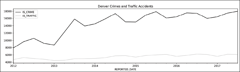
Quarterly crime plot
How it works…
After reading in and preparing our data in step 1, we begin grouping and aggregating in step 2. Immediately after calling the .resample method, we can continue either by chaining a method or by selecting a group of columns to aggregate. We choose to select the IS_CRIME and IS_TRAFFIC columns to aggregate. If we didn't select just these two, then all of the numeric columns would have been summed with the following outcome:
>>> (crime
...     .resample('Q')
...     .sum()
... )
                    GEO_LON  ...  IS_TRAFFIC
REPORTED_DATE                ...
2012-03-31    -1.313006e+06  ...        4726
2012-06-30    -1.547274e+06  ...        5255
2012-09-30    -1.615835e+06  ...        5003
2012-12-31    -1.458177e+06  ...        4802
2013-03-31    -1.368931e+06  ...        4442
...                     ...  ...         ...
2016-09-30    -2.459343e+06  ...        6199
2016-12-31    -2.293628e+06  ...        6094
2017-03-31    -2.288383e+06  ...        5587
2017-06-30    -2.453857e+06  ...        6148
2017-09-30    -2.508001e+06  ...        6101
By default, the offset alias Q technically uses December 31st as the last day of the year. The span of dates that represent a single quarter are all calculated using this ending date. The aggregated result uses the last day of the quarter as its label. Step 3 uses the offset alias QS, which, by default, calculates quarters using January 1st as the first day of the year.
Most public businesses report quarterly earnings but they do not all have the same calendar year beginning in January. For instance, if we wanted our quarters to begin March 1st, then we could use QS-MAR to anchor our offset alias:
>>> (crime_sort
...     .resample('QS-MAR')
...     [['IS_CRIME', 'IS_TRAFFIC']]
...     .sum()
... )
               IS_CRIME  IS_TRAFFIC
REPORTED_DATE
2011-12-01         5013        3198
2012-03-01         9260        4954
2012-06-01        10524        5190
2012-09-01         9450        4777
2012-12-01         9003        4652
...                 ...         ...
2016-09-01        16932        6202
2016-12-01        15615        5731
2017-03-01        17287        5940
2017-06-01        18545        6246
2017-09-01         5417        1931
As in the preceding recipe, we verify our results via manual slicing in step 4. In step 5 we replicate the result of step 3 with the .groupby method using pd.Grouper to set our group length. In step 6, we call the DataFrame .plot method. By default, a line is plotted for each column of data. The plot clearly shows a sharp increase in reported crimes during the first three quarters of the year. There also appears to be a seasonal component to both crime and traffic, with numbers lower in the cooler months and higher in the warmer months.
There's more…
To get a different visual perspective, we can plot the percentage increase in crime and traffic, instead of the raw count. Let's divide all the data by the first row and plot again:
>>> crime_begin = (crime
...     .resample('Q')
...     [['IS_CRIME', 'IS_TRAFFIC']]
...     .sum()
...     .iloc[0]
... )
>>> fig, ax = plt.subplots(figsize=(16, 4))
>>> (crime
...     .resample('Q')
...     [['IS_CRIME', 'IS_TRAFFIC']]
...     .sum()
...     .div(crime_begin)
...     .sub(1)
...     .round(2)
...     .mul(100)
...     .plot.bar(color=['black', 'lightgrey'], ax=ax,
...           title='Denver Crimes and Traffic Accidents % Increase')
... )
>>> fig.autofmt_xdate()
>>> fig.savefig('c12-crimes3.png', dpi=300, bbox_inches='tight')
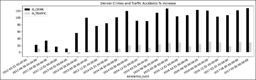
Quarterly crime plot
Measuring crime by weekday and year
Measuring crimes by weekday and by year simultaneously requires the functionality to pull this information from a Timestamp. Thankfully, this functionality is built into any Timestamp column with the .dt attribute.
In this recipe, we will use the .dt attribute to provide us with both the weekday name and year of each crime as a Series. We count all of the crimes by forming groups using both of these Series. Finally, we adjust the data to consider partial years and population before creating a heatmap of the total amount of crime.
How to do it…
- Read in the Denver crime hdf5 dataset leaving the
REPORTED_DATEas a column:>>> crime = pd.read_hdf('data/crime.h5', 'crime') >>> crime OFFEN/PE_ID ... IS_TRAFFIC 0 traffic-accident-dui-duid ... 1 1 vehicular-eluding-no-chase ... 0 2 disturbing-the-peace ... 0 3 curfew ... 0 4 aggravated-assault ... 0 ... ... ... ... 460906 burglary-business-by-force ... 0 460907 weapon-unlawful-discharge-of ... 0 460908 traf-habitual-offender ... 0 460909 criminal-mischief-other ... 0 460910 theft-other ... 0 - All Timestamp columns have a special attribute,
.dt, which gives access to a variety of extra attributes and methods specifically designed for dates. Let's find the day name of eachREPORTED_DATEand then count these values:>>> (crime ... ['REPORTED_DATE'] ... .dt.day_name() ... .value_counts() ... ) Monday 70024 Friday 69621 Wednesday 69538 Thursday 69287 Tuesday 68394 Saturday 58834 Sunday 55213 Name: REPORTED_DATE, dtype: int64 - The weekends appear to have substantially less crime and traffic accidents. Let's put this data in correct weekday order and make a horizontal bar plot:
>>> days = ['Monday', 'Tuesday', 'Wednesday', 'Thursday',
...         'Friday', 'Saturday', 'Sunday']
>>> title = 'Denver Crimes and Traffic Accidents per Weekday'
>>> fig, ax = plt.subplots(figsize=(6, 4))
>>> (crime
...    ['REPORTED_DATE']
...    .dt.day_name()
...    .value_counts()
...    .reindex(days)
...    .plot.barh(title=title, ax=ax)
... )
>>> fig.savefig('c12-crimes4.png', dpi=300, bbox_inches='tight')
Weekday crime plot
- We can do a very similar procedure to plot the count by year:
>>> title = 'Denver Crimes and Traffic Accidents per Year'
>>> fig, ax = plt.subplots(figsize=(6, 4))
>>> (crime
...    ['REPORTED_DATE']
...    .dt.year
...    .value_counts()
...    .sort_index()
...    .plot.barh(title=title, ax=ax)
... )
>>> fig.savefig('c12-crimes5.png', dpi=300, bbox_inches='tight')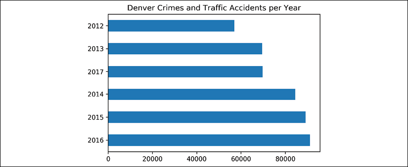
Yearly crime plot
- We need to group by both weekday and year. One way of doing this is to use these attributes in the
.groupbymethod:>>> (crime ... .groupby([crime['REPORTED_DATE'].dt.year.rename('year'), ... crime['REPORTED_DATE'].dt.day_name().rename('day')]) ... .size() ... ) year day 2012 Friday 8549 Monday 8786 Saturday 7442 Sunday 7189 Thursday 8440 ... 2017 Saturday 8514 Sunday 8124 Thursday 10545 Tuesday 10628 Wednesday 10576 Length: 42, dtype: int64 - We have aggregated the data correctly, but the structure is not conducive to make comparisons easily. Let's use the
.unstackmethod to get a more readable table:>>> (crime ... .groupby([crime['REPORTED_DATE'].dt.year.rename('year'), ... crime['REPORTED_DATE'].dt.day_name().rename('day')]) ... .size() ... .unstack('day') ... ) day Friday Monday Saturday Sunday Thursday Tuesday year 2012 8549 8786 7442 7189 8440 8191 2013 10380 10627 8875 8444 10431 10416 2014 12683 12813 10950 10278 12309 12440 2015 13273 13452 11586 10624 13512 13381 2016 14059 13708 11467 10554 14050 13338 2017 10677 10638 8514 8124 10545 10628 - We now have a nicer representation that is easier to read but noticeably, the 2017 numbers are incomplete. To help make a fairer comparison, we can make a linear extrapolation to estimate the final number of crimes. Let's first find the last day that we have data for in 2017:
>>> criteria = crime['REPORTED_DATE'].dt.year == 2017 >>> crime.loc[criteria, 'REPORTED_DATE'].dt.dayofyear.max() 272 - A naive estimate would be to assume a constant rate of crime throughout the year and multiply all values in the 2017 table by 365/272. However, we can do a little better and look at our historical data and calculate the average percentage of crimes that have taken place through the first 272 days of the year:
>>> round(272 / 365, 3) 0.745 >>> crime_pct = (crime ... ['REPORTED_DATE'] ... .dt.dayofyear.le(272) ... .groupby(crime.REPORTED_DATE.dt.year) ... .mean() ... .mul(100) ... .round(2) ... ) >>> crime_pct REPORTED_DATE 2012 74.84 2013 72.54 2014 75.06 2015 74.81 2016 75.15 2017 100.00 Name: REPORTED_DATE, dtype: float64 >>> crime_pct.loc[2012:2016].median() 74.84 - It turns out (perhaps coincidentally) that the percentage of crimes that happen during the first 272 days of the year is almost exactly proportional to the percentage of days passed in the year. Let's now update the row for 2017 and change the column order to match the weekday order:
>>> def update_2017(df_): ... df_.loc[2017] = (df_ ... .loc[2017] ... .div(.748) ... .astype('int') ... ) ... return df_ >>> (crime ... .groupby([crime['REPORTED_DATE'].dt.year.rename('year'), ... crime['REPORTED_DATE'].dt.day_name().rename('day')]) ... .size() ... .unstack('day') ... .pipe(update_2017) ... .reindex(columns=days) ... ) day Monday Tuesday Wednesday ... Friday Saturday Sunday year ... 2012 8786 8191 8440 ... 8549 7442 7189 2013 10627 10416 10354 ... 10380 8875 8444 2014 12813 12440 12948 ... 12683 10950 10278 2015 13452 13381 13320 ... 13273 11586 10624 2016 13708 13338 13900 ... 14059 11467 10554 2017 14221 14208 14139 ... 14274 11382 10860 - We could make a bar or line plot, but this is also a good situation for a heatmap, which is in the
seabornlibrary:>>> import seaborn as sns >>> fig, ax = plt.subplots(figsize=(6, 4)) >>> table = (crime ... .groupby([crime['REPORTED_DATE'].dt.year.rename('year'), ... crime['REPORTED_DATE'].dt.day_name().rename('day')]) ... .size() ... .unstack('day') ... .pipe(update_2017) ... .reindex(columns=days) ... ) >>> sns.heatmap(table, cmap='Greys', ax=ax) >>> fig.savefig('c12-crimes6.png', dpi=300, bbox_inches='tight')
Yearly crime heatmap
- Crime seems to be rising every year but this data does not account for rising population. Let's read in a table for the Denver population for each year that we have data:
>>> denver_pop = pd.read_csv('data/denver_pop.csv', ... index_col='Year') >>> denver_pop Population Year 2017 705000 2016 693000 2015 680000 2014 662000 2013 647000 2012 634000 - Many crime metrics are reported as rates per 100,000 residents. Let's divide the population by 100,000 and then divide the raw crime counts by this number to get the crime rate per 100,000 residents:
>>> den_100k = denver_pop.div(100_000).squeeze() >>> normalized = (crime ... .groupby([crime['REPORTED_DATE'].dt.year.rename('year'), ... crime['REPORTED_DATE'].dt.day_name().rename('day')]) ... .size() ... .unstack('day') ... .pipe(update_2017) ... .reindex(columns=days) ... .div(den_100k, axis='index') ... .astype(int) ... ) >>> normalized day Monday Tuesday Wednesday ... Friday Saturday Sunday 2012 1385 1291 1331 ... 1348 1173 1133 2013 1642 1609 1600 ... 1604 1371 1305 2014 1935 1879 1955 ... 1915 1654 1552 2015 1978 1967 1958 ... 1951 1703 1562 2016 1978 1924 2005 ... 2028 1654 1522 2017 2017 2015 2005 ... 2024 1614 1540 - Once again, we can make a heatmap that, even after adjusting for population increase, looks nearly identical to the first one:
>>> import seaborn as sns
>>> fig, ax = plt.subplots(figsize=(6, 4))
>>> sns.heatmap(normalized, cmap='Greys', ax=ax)
>>> fig.savefig('c12-crimes7.png', dpi=300, bbox_inches='tight')
Normalized yearly crime heatmap
How it works…
All DataFrame columns containing Timestamps have access to numerous other attributes and methods with the .dt attribute. In fact, all of these methods and attributes available from the .dt attribute are also available on a Timestamp object.
In step 2, we use the .dt attribute (which only works on a Series) to extract the day name and count the occurrences. Before making a plot in step 3, we manually rearrange the order of the index with the .reindex method, which, in its most basic use case, accepts a list containing the desired order. This task could have also been accomplished with the .loc indexer like this:
>>> (crime
...    ['REPORTED_DATE']
...    .dt.day_name()
...    .value_counts()
...    .loc[days]
... )
Monday       70024
Tuesday      68394
Wednesday    69538
Thursday     69287
Friday       69621
Saturday     58834
Sunday       55213
Name: REPORTED_DATE, dtype: int64
The .reindex method is more performant and has many parameters for more diverse situations than .loc.
In step 4, we do a very similar procedure and retrieve the year using the .dt attribute again, and then count the occurrences with the .value_counts method. In this instance, we use .sort_index over .reindex, as years will naturally sort in the desired order.
The goal of the recipe is to group by both weekday and year together, which we do in step 5. The .groupby method is flexible and can form groups in multiple ways. In this recipe, we pass it two Series derived from the year and weekday columns. We then chain the .size method to it, which returns a single value, the length of each group.
After step 5, our Series is long with only a single column of data, which makes it difficult to make comparisons by year and weekday.
To ease the readability, we pivot the weekday level into horizontal column names with .unstack in step 6. Step 6 is doing a cross tabulation. Here is another way to do this in pandas:
>>> (crime
...     .assign(year=crime.REPORTED_DATE.dt.year,
...             day=crime.REPORTED_DATE.dt.day_name())
...     .pipe(lambda df_: pd.crosstab(df_.year, df_.day))
... )
day   Friday  Monday  ...  Tuesday  Wednesday
year                  ...
2012    8549    8786  ...     8191       8440
2013   10380   10627  ...    10416      10354
2014   12683   12813  ...    12440      12948
2015   13273   13452  ...    13381      13320
2016   14059   13708  ...    13338      13900
2017   10677   10638  ...    10628      10576
In step 7, we use Boolean indexing to select only the crimes in 2017 and then use .dayofyear from the .dt attribute to find the total elapsed days from the beginning of the year. The maximum of this Series should tell us how many days we have data for in 2017.
Step 8 is quite complex. We first create a Boolean Series by testing whether each crime was committed on or before the 272nd day of the year with crime['REPORTED_DATE'].dt.dayofyear.le(272). From here, we again use the .groupby method to form groups by the previously calculated year Series and then use the .mean method to find the percentage of crimes committed on or before the 272nd day for each year.
The .loc attribute selects the entire 2017 row of data in step 9. We adjust this row by dividing by the median percentage found in step 8.
Lots of crime visualizations are done with heatmaps, and one is done here in step 10 with the help of the seaborn library. The cmap parameter takes a string name of the several dozen available matplotlib colormaps.
In step 12, we create a crime rate per 100k residents by dividing by the population of that year. This is another fairly tricky operation. Normally, when you divide one DataFrame by another, they align on their columns and index. However, in this step, there are no columns in common with denver_pop so no values will align if we try and divide them. To work around this, we create the den_100k Series with the squeeze method. We still can't divide these two objects as, by default, division between a DataFrame and a Series aligns the columns of the DataFrame with the index of the Series, like this:
>>> (crime
...     .groupby([crime['REPORTED_DATE'].dt.year.rename('year'),
...               crime['REPORTED_DATE'].dt.day_name().rename('day')])
...     .size()
...     .unstack('day')
...     .pipe(update_2017)
...     .reindex(columns=days)
... ) / den_100k
      2012  2013  2014  ...  Thursday  Tuesday  Wednesday
year                    ...
2012   NaN   NaN   NaN  ...       NaN      NaN       NaN
2013   NaN   NaN   NaN  ...       NaN      NaN       NaN
2014   NaN   NaN   NaN  ...       NaN      NaN       NaN
2015   NaN   NaN   NaN  ...       NaN      NaN       NaN
2016   NaN   NaN   NaN  ...       NaN      NaN       NaN
2017   NaN   NaN   NaN  ...       NaN      NaN       NaN
We need the index of the DataFrame to align with the index of Series, and to do this, we use the .div method, which allows us to change the direction of alignment with the axis parameter. A heatmap of the adjusted crime rate is plotted in step 13.
There's more…
If we wanted to look at specific types of crimes we could do the following:
>>> days = ['Monday', 'Tuesday', 'Wednesday', 'Thursday',
...         'Friday', 'Saturday', 'Sunday']
>>> crime_type = 'auto-theft'
>>> normalized = (crime
...     .query('OFFENSE_CATEGORY_ID == @crime_type')
...     .groupby([crime['REPORTED_DATE'].dt.year.rename('year'),
...               crime['REPORTED_DATE'].dt.day_name().rename('day')])
...     .size()
...     .unstack('day')
...     .pipe(update_2017)
...     .reindex(columns=days)
...     .div(den_100k, axis='index')
...     .astype(int)
... )
>>> normalized
day   Monday  Tuesday  Wednesday  ...  Friday  Saturday  Sunday
2012      95       72         72  ...      71        78      76
2013      85       74         74  ...      65        68      67
2014      94       76         72  ...      76        67      67
2015     108      102         89  ...      92        85      78
2016     119      102        100  ...      97        86      85
2017     114      118        111  ...     111        91     102
Grouping with anonymous functions with a DatetimeIndex
Using DataFrames with a DatetimeIndex opens the door to many new and different operations as seen with several recipes in this chapter.
In this recipe, we will show the versatility of using the .groupby method for DataFrames that have a DatetimeIndex.
How to do it…
- Read in the Denver crime hdf5 file, place the
REPORTED_DATEcolumn in the index, and sort it:>>> crime = (pd.read_hdf('data/crime.h5', 'crime') ... .set_index('REPORTED_DATE') ... .sort_index() ... ) - The
DatetimeIndexhas many of the same attributes and methods as a pandasTimestamp. Let's take a look at some that they have in common:>>> common_attrs = (set(dir(crime.index)) & ... set(dir(pd.Timestamp))) >>> [attr for attr in common_attrs if attr[0] != '_'] ['tz_convert', 'is_month_start', 'nanosecond', 'day_name', 'microsecond', 'quarter', 'time', 'tzinfo', 'week', 'year', 'to_period', 'freqstr', 'dayofyear', 'is_year_end', 'weekday_name', 'month_name', 'minute', 'hour', 'dayofweek', 'second', 'max', 'min', 'to_numpy', 'tz_localize', 'is_quarter_end', 'to_julian_date', 'strftime', 'day', 'days_in_month', 'weekofyear', 'date', 'daysinmonth', 'month', 'weekday', 'is_year_start', 'is_month_end', 'ceil', 'timetz', 'freq', 'tz', 'is_quarter_start', 'floor', 'normalize', 'resolution', 'is_leap_year', 'round', 'to_pydatetime'] - We can then use the
.indexto find weekday names, similarly to what was done in step 2 of the preceding recipe:>>> crime.index.day_name().value_counts() Monday 70024 Friday 69621 Wednesday 69538 Thursday 69287 Tuesday 68394 Saturday 58834 Sunday 55213 Name: REPORTED_DATE, dtype: int64 - The
.groupbymethod can accept a function as an argument. This function will be passed the.indexand the return value is used to form groups. Let's see this in action by grouping with a function that turns the.indexinto a weekday name and then counts the number of crimes and traffic accidents separately:>>> (crime ... .groupby(lambda idx: idx.day_name()) ... [['IS_CRIME', 'IS_TRAFFIC']] ... .sum() ... ) IS_CRIME IS_TRAFFIC Friday 48833 20814 Monday 52158 17895 Saturday 43363 15516 Sunday 42315 12968 Thursday 49470 19845 Tuesday 49658 18755 Wednesday 50054 19508 - You can use a list of functions to group by both the hour of day and year, and then reshape the table to make it more readable:
>>> funcs = [lambda idx: idx.round('2h').hour, lambda idx: idx.year] >>> (crime ... .groupby(funcs) ... [['IS_CRIME', 'IS_TRAFFIC']] ... .sum() ... .unstack() ... ) IS_CRIME ... IS_TRAFFIC 2012 2013 2014 ... 2015 2016 2017 0 2422 4040 5649 ... 1136 980 782 2 1888 3214 4245 ... 773 718 537 4 1472 2181 2956 ... 471 464 313 6 1067 1365 1750 ... 494 593 462 8 2998 3445 3727 ... 2331 2372 1828 .. ... ... ... ... ... ... ... 14 4266 5698 6708 ... 2840 2763 1990 16 4113 5889 7351 ... 3160 3527 2784 18 3660 5094 6586 ... 3412 3608 2718 20 3521 4895 6130 ... 2071 2184 1491 22 3078 4318 5496 ... 1671 1472 1072 - If you are using Jupyter, you can add
.style.highlight_max(color='lightgrey')to bring attention to the largest value in each column:>>> funcs = [lambda idx: idx.round('2h').hour, lambda idx: idx.year] >>> (crime ... .groupby(funcs) ... [['IS_CRIME', 'IS_TRAFFIC']] ... .sum() ... .unstack() ... .style.highlight_max(color='lightgrey') ... )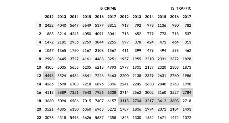
Popular crime hours
How it works…
In step 1, we read in our data and placed a Timestamp column into the index to create a DatetimeIndex. In step 2, we see that a DatetimeIndex has lots of the same functionality that a single Timestamp object has. In step 3, we use these extra features of the DatetimeIndex to extract the day name.
In step 4, we take advantage of the .groupby method to accept a function that is passed the DatetimeIndex. The idx in the anonymous function is the DatetimeIndex, and we use it to retrieve the day name. It is possible to pass .groupby a list of any number of custom functions, as done in step 5. Here, the first function uses the .round DatetimeIndex method to round each value to the nearest second hour. The second function returns the .year attribute. After the grouping and aggregating, we .unstack the years as columns. We then highlight the maximum value of each column. Crime is reported most often between 3 and 5 P.M. Most traffic accidents occur between 5 P.M. and 7 P.M.
Grouping by a Timestamp and another column
The .resample method is unable to group by anything other than periods of time. The .groupby method, however, has the ability to group by both periods of time and other columns.
In this recipe, we will show two very similar but different approaches to group by Timestamps and another column.
How to do it…
- Read in the employee dataset, and create a
DatetimeIndexwith theHIRE_DATEcolumn:>>> employee = pd.read_csv('data/employee.csv', ... parse_dates=['JOB_DATE', 'HIRE_DATE'], ... index_col='HIRE_DATE') >>> employee UNIQUE_ID ... JOB_DATE HIRE_DATE ... 2006-06-12 0 ... 2012-10-13 2000-07-19 1 ... 2010-09-18 2015-02-03 2 ... 2015-02-03 1982-02-08 3 ... 1991-05-25 1989-06-19 4 ... 1994-10-22 ... ... ... ... 2014-06-09 1995 ... 2015-06-09 2003-09-02 1996 ... 2013-10-06 2014-10-13 1997 ... 2015-10-13 2009-01-20 1998 ... 2011-07-02 2009-01-12 1999 ... 2010-07-12 - Let's first do a grouping by just gender, and find the average salary for each:
>>> (employee ... .groupby('GENDER') ... ['BASE_SALARY'] ... .mean() ... .round(-2) ... ) GENDER Female 52200.0 Male 57400.0 Name: BASE_SALARY, dtype: float64 - Let's find the average salary based on hire date, and group everyone into 10-year buckets:
>>> (employee ... .resample('10AS') ... ['BASE_SALARY'] ... .mean() ... .round(-2) ... ) HIRE_DATE 1958-01-01 81200.0 1968-01-01 106500.0 1978-01-01 69600.0 1988-01-01 62300.0 1998-01-01 58200.0 2008-01-01 47200.0 Freq: 10AS-JAN, Name: BASE_SALARY, dtype: float64 - If we wanted to group by both gender and a ten-year time span, we can call
.resampleafter calling.groupby:>>> (employee ... .groupby('GENDER') ... .resample('10AS') ... ['BASE_SALARY'] ... .mean() ... .round(-2) ... ) GENDER HIRE_DATE Female 1975-01-01 51600.0 1985-01-01 57600.0 1995-01-01 55500.0 2005-01-01 51700.0 2015-01-01 38600.0 ... Male 1968-01-01 106500.0 1978-01-01 72300.0 1988-01-01 64600.0 1998-01-01 59700.0 2008-01-01 47200.0 Name: BASE_SALARY, Length: 11, dtype: float64 - Now, this does what we set out to do, but we run into a slight issue whenever we want to compare female to male salaries. Let's
.unstackthe gender level and see what happens:>>> (employee ... .groupby('GENDER') ... .resample('10AS') ... ['BASE_SALARY'] ... .mean() ... .round(-2) ... .unstack('GENDER') ... ) GENDER Female Male HIRE_DATE 1958-0... NaN 81200.0 1968-0... NaN 106500.0 1975-0... 51600.0 NaN 1978-0... NaN 72300.0 1985-0... 57600.0 NaN ... ... ... 1995-0... 55500.0 NaN 1998-0... NaN 59700.0 2005-0... 51700.0 NaN 2008-0... NaN 47200.0 2015-0... 38600.0 NaN - The 10-year periods for males and females do not begin on the same date. This happened because the data was first grouped by gender and then, within each gender, more groups were formed based on hire dates. Let's verify that the first hired male was in 1958 and the first hired female was in 1975:
>>> employee[employee['GENDER'] == 'Male'].index.min() Timestamp('1958-12-29 00:00:00') >>> employee[employee['GENDER'] == 'Female'].index.min() Timestamp('1975-06-09 00:00:00') - To resolve this issue, we must group the date together with the gender, and this is only possible with the
.groupbymethod:>>> (employee ... .groupby(['GENDER', pd.Grouper(freq='10AS')]) ... ['BASE_SALARY'] ... .mean() ... .round(-2) ... ) GENDER HIRE_DATE Female 1968-01-01 NaN 1978-01-01 57100.0 1988-01-01 57100.0 1998-01-01 54700.0 2008-01-01 47300.0 ... Male 1968-01-01 106500.0 1978-01-01 72300.0 1988-01-01 64600.0 1998-01-01 59700.0 2008-01-01 47200.0 Name: BASE_SALARY, Length: 11, dtype: float64 - Now we can
.unstackthe gender and get our rows aligned perfectly:>>> (employee ... .groupby(['GENDER', pd.Grouper(freq='10AS')]) ... ['BASE_SALARY'] ... .mean() ... .round(-2) ... .unstack('GENDER') ... ) GENDER Female Male HIRE_DATE 1958-0... NaN 81200.0 1968-0... NaN 106500.0 1978-0... 57100.0 72300.0 1988-0... 57100.0 64600.0 1998-0... 54700.0 59700.0 2008-0... 47300.0 47200.0
How it works…
The read_csv function in step 1 allows to both convert columns into Timestamps and put them in the index at the same time creating a DatetimeIndex. Step 2 does a .groupby operation with a single grouping column, gender. Step 3 uses the .resample method with the offset alias 10AS to form groups in 10-year increments of time. The A is the alias for year, and the S informs us that the beginning of the period is used as the label. For instance, the data for the label 1988-01-01 spans that date until December 31, 1997.
In step 4, for each gender, male and female, completely different starting dates for the 10-year periods are calculated based on the earliest hired employee. Step 5 shows how this causes misalignment when we try to compare salaries of females to males. They don't have the same 10-year periods. Step 6 verifies that the year of the earliest hired employee for each gender matches the output from step 4.
To alleviate this issue, we must group both the gender and Timestamp together. The .resample method is only capable of grouping by a single column of Timestamps. We can only complete this operation with the .groupby method. With pd.Grouper, we can replicate the functionality of .resample. We pass the offset alias to the freq parameter and then place the object in a list with all the other columns that we wish to group, as done in step 7.
As both males and females now have the same starting dates for the 10-year period, the reshaped data in step 8 will align for each gender making comparisons much easier. It appears that male salaries tend to be higher given a longer length of employment, though both genders have the same average salary with under ten years of employment.
There's more…
From an outsider's perspective, it would not be obvious that the rows from the output in step 8 represented 10-year intervals. One way to improve the index labels would be to show the beginning and end of each time interval. We can achieve this by concatenating the current index year with 9 added to itself:
>>> sal_final = (employee
...    .groupby(['GENDER', pd.Grouper(freq='10AS')])
...    ['BASE_SALARY']
...    .mean()
...    .round(-2)
...    .unstack('GENDER')
... )
>>> years = sal_final.index.year
>>> years_right = years + 9
>>> sal_final.index = years.astype(str) + '-' + years_right.astype(str)
>>> sal_final
GENDER      Female      Male
HIRE_DATE
1958-1967      NaN   81200.0
1968-1977      NaN  106500.0
1978-1987  57100.0   72300.0
1988-1997  57100.0   64600.0
1998-2007  54700.0   59700.0
2008-2017  47300.0   47200.0
There is a completely different way to do this recipe. We can use the cut function to create equal-width intervals based on the year that each employee was hired and form groups from it:
>>> cuts = pd.cut(employee.index.year, bins=5, precision=0)
>>> cuts.categories.values
IntervalArray([(1958.0, 1970.0], (1970.0, 1981.0], (1981.0, 1993.0], (1993.0, 2004.0], (2004.0, 2016.0]],
closed='right',
dtype='interval[float64]')
>>> (employee
...     .groupby([cuts, 'GENDER'])
...     ['BASE_SALARY']
...     .mean()
...     .unstack('GENDER')
...     .round(-2)
... )
GENDER             Female     Male
(1958.0, 1970.0]      NaN  85400.0
(1970.0, 1981.0]  54400.0  72700.0
(1981.0, 1993.0]  55700.0  69300.0
(1993.0, 2004.0]  56500.0  62300.0
(2004.0, 2016.0]  49100.0  49800.0