
Chapter 6
Where to Parallelize
What's in This Chapter?
Hotspot analysis using the Intel compiler
Hotspot analysis using the auto-parallelizer
Hotspot analysis using Amplifier XE
The purpose of parallelization is to improve the performance of an application. Performance can be measured either by how much time a program takes to run or by how much work a program can do per second. Within a program, it is the busy sections, or hotspots, that should be made parallel. The more the hotspots contribute to the overall run time of the program, the better the performance improvement you will obtain by parallelizing them.
Hotspot analysis is an important first step in the parallelism process. This chapter shows three different ways to identify hotspots in your code using Parallel Studio XE. Without carrying out Hotspot analysis, there is a danger that you will end up making little or no difference to your program's performance. The section “Hotspot Analysis Using the Auto-Parallelizer” includes some tips on how to help the auto-parallelizer do its job better.
map_opts -tl -lc -opts /Oy-
Intel(R) Compiler option mapping tool

mapping Windows options to Linux for C++

‘-Oy-’ Windows option maps to
  --> ‘-fomit-frame-pointer-’ option on Linux
  --> ‘-fno-omit-frame-pointer’ option on Linux
  --> ‘-fp’ option on Linux
Different Ways of Profiling
You are already familiar with the four steps to parallelization (described in Chapter 3, “Parallel Studio XE for the Impatient”): analyze, implement, debug, and tune. It's now time to carry out the first of those steps, analyzing the hotspots in your code.
This book describes four ways of conducting a Hotspot analysis, the first three of which are covered in this chapter:
- Using the Intel compiler's loop profiler and associated profile viewer
- Letting the Intel compiler's auto-parallelizer help you find the hotspots
- Using Amplifier XE
- Performing a survey using Advisor (covered in Chapter 10, “Parallel Advisor Driven Design”)
Each approach has its merits, and you will probably grow to like a particular one. What you shouldn't do is guess where the hotspots are! If you do, you could end up spending wasted effort making code parallel with little or no return on your invested time.
The Example Application
The code in Listing 6.1 (at the end of this chapter) produces a black-and-white picture of a Mandelbrot fractal. The picture is stored as a PPM file and can be viewed with any PPM viewer. If you don't have a viewer, try IrfanView (www.irfanview.com).
Listing 6.1 is split into the following files:
- main.cpp — The entry point to the program
- mandelbrot.cpp — Calculates the fractal
- mandelbrot.h — Contains a number of defines and prototypes
- ppm.cpp — Prints the fractal to a PPM file
- wtime.c — A utility for measuring the application run time
When you run the example application, it displays the following simple text on the screen:
calculating…
printing…
Time to calc :…3.707
Time to print :…7.548
Time (Total) :…11.25
Figure 6.1 shows the default.ppm file generated by running the application and viewed using IrfanView.
Figure 6.1 The output of the Mandelbrot application
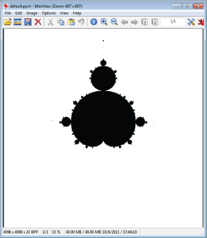
Table 6.1 shows the results of running the program built with the Intel compiler, using the options /O2 (optimize for speed) and /Qipo (enable interprocedural optimization). The results are the best of five runs, on an Intel Xeon Workstation with an Intel Xeon CPU, X5680 @ 3.33 GHz (two processors, supporting a total of 24 hardware threads).
Table 6.1 Time Taken to Run the Example Application
| Function | Time |
| Calculating | 3.433 |
| Printing | 2.206 |
| Total | 5.638 |
icl /O2 /Qipo wtime.c main.cpp mandelbrot.cpp ppm.cpp -o 6-1.exe
6-1.exe
Instructions for Linux Users
Sourcing the Compiler and Amplifier XE
source /opt/intel/composerxe/bin/compilervars.sh intel64
source /opt/intel/vtune_amplifier_xe/amplxe-vars.sh
source /opt/intel/inspector_xe/inspxe-vars.sh
Viewing the PPM File
Hotspot Analysis Using the Intel Compiler
A well-kept secret is that the Intel compiler has its own profiler and viewer. These are different products from Amplifier XE and rely on the compiler instrumenting your code.
With the profiler and viewer you can:
- Profile functions
- Profile loops
- View the output in a standalone viewer
- Read the results from a text file
Profiling Steps
Figure 6.2 shows the steps for profiling an application:
If you do not want to use the profile viewer or the XML, you can read the results from the .dump file. You can disable the generating of an XML file by setting the INTEL_LOOP_PROF_XML_DUMP environment variable to zero. Table 6.2 lists the options for controlling the profiling.
- Don't use IPO. You can disable it with the compiler option /Qipo-.
- Disable inlining using the /Ob0 or /Ob1 option.
- Use the /Qopt-report-phase ipo_inl option to get a list of inlined functions so that you can manually reconstruct the call tree.
Figure 6.2 Using the Intel compiler to find the hotspots
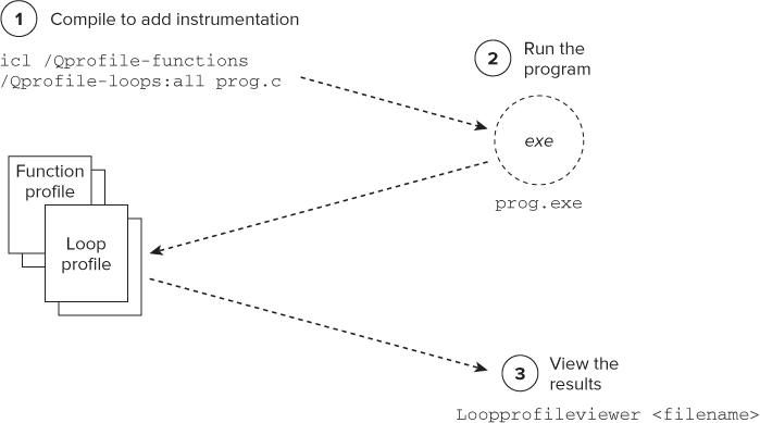
Table 6.2 Profiling Options and Their Arguments
| Option | Arguments |
| /Qprofile-functions | None |
| /Qprofile-loops:<arg> | Inner, outer, all |
| /Qprofile-loops-report:<arg> | 1 or 2 (times, or times and counts) |
An Example Session
Taking the Mandelbrot program, which by now you should be familiar with, here is a description of the profiling steps and the output generated. You can try this for yourself in Activity 6-2.
icl /Zi /O2 /Qipo wtime.c main.cpp  mandelbrot.cpp  ppm.cpp -o m1.exe
   /Qprofile-functions  /Qprofile-loops:all /Qprofile-loops-report:2
C:>m1.exe
calculating…
printing…
Time to calc :…3.707
Time to print :…7.548
Time (Total) :…11.25
C:dvCH6>dir /b
default.ppm
loop_prof_1317923290.xml
loop_prof_funcs_1317923290.dump
loop_prof_loops_1317923290.dump
m1.exe
m1.ilk
m1.pdb
main.cpp
main.obj
mandelbrot.cpp
mandelbrot.h
mandelbrot.obj
ppm.cpp
ppm.obj
vc90.pdb
loopprofileviewer  loop_prof_1317923290.xml

(Linux users: loopprofileviewer.sh or loopprofileviewer.csh)
-> INLINE: ?Mandelbrot@@YAXXZ(2905) (isz = 71) (sz = 74 (31+43))
    -> INLINE: ?SetZ@@YAXHHMM@Z(2906) (isz = 51) (sz = 62 (19+43))
      -> INLINE: ?CalcMandelbrot@@YAMMM@Z(2907) (isz = 26) (sz = 36 (17+19))
- There should be a decent number of iterations of the loop.
- The individual loops should do a reasonable amount of work.
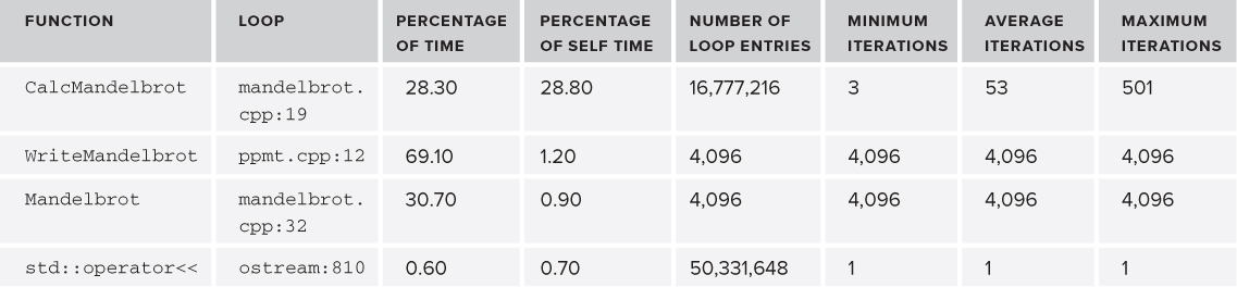
Figure 6.3 The standalone loop-profiling viewer
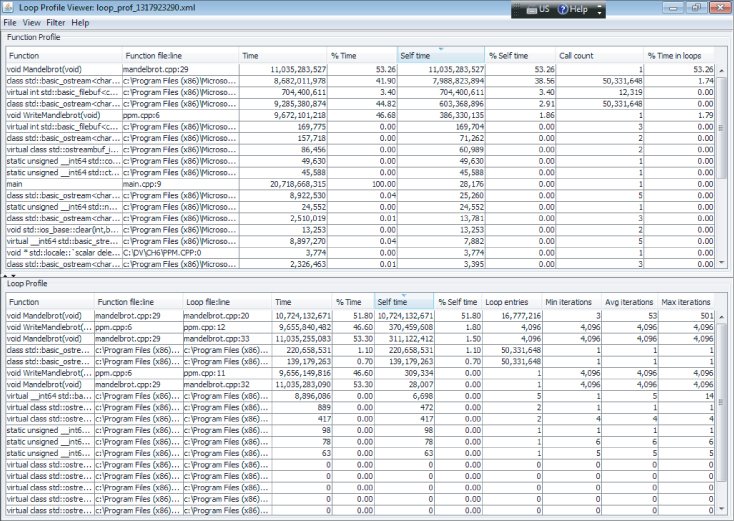
Table 6.3 Results of the Loop Profiling with Inlining Enabled
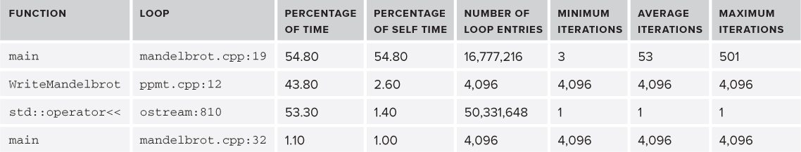
Table 6.4 Results of the Loop Profiling with Inlining Enabled
Overhead Introduced by Profiling
Using the profiling option of the compiler adds an overhead to the run time. Table 6.5 records the time taken for each type of profiling. On the Mandelbrot program, with all the profiling options enabled, the program runs twice as slow as when no profiling is carried out.
- Pros
- Easy to use
- Everything you need is available with the compiler, including a standalone viewer
- Profiles loops as well as functions
- Cons
- Very basic functionality
- Requires code to be instrumented, introducing a compile-time and a runtime overhead, which can be significant
- No call tree, so you have to construct the call stack manually
- No comparison facility
Table 6.5 Time Taken to Run the Example Application
| Type of Profiling | Time | Speedup |
| No profiling | 5.638 | 1 |
| Functions | 7.953 | 0.71 |
| Functions and outer loops (time) | 10.68 | 0.53 |
| Functions and outer loops (time and count) | 10.86 | 0.52 |
| Functions and all loops (time) | 10.98 | 0.51 |
| Functions and all loops (time and count) | 11.25 | 0.50 |
icl /Zi /O2 /Qipo wtime.c main.cpp  mandelbrot.cpp  ppm.cpp -o 6-2.exe
    /Qprofile-functions  /Qprofile-loops:all /Qprofile-loops-report:2
6-2.exe
Dealing with the Lack of Symbol Visibility
icl /Zi /O2 /Qipo wtime.c main.cpp  mandelbrot.cpp  ppm.cpp -o 6-2.exe
   /Qprofile-functions  /Qprofile-loops:all
/Qprofile-loops-report:2  /Qopt-report-phase ipo_inl
/Qopt-report-routine:main
Instructions for Linux Users
Hotspot Analysis Using the Auto-Parallelizer
The Intel compiler has an auto-parallelizer that can automatically add parallelism to loops. By default, the auto-parallelizer is disabled, but you can enable it with the /Qparallel option. Some developers use this feature to give hints on where best to parallelize their code.
The auto-parallelizer does four things:
- Finds loops that could be candidates for making parallel
- Decides if there is a sufficient amount of work done to justify parallelization
- Checks that no loop dependencies exist
- Appropriately partitions any data between the parallelized code
Profiling Steps
Figure 6.4 shows the steps for profiling with the help of the auto-parallelizer:
Figure 6.4 Using the auto-parallelizer to find hotspots
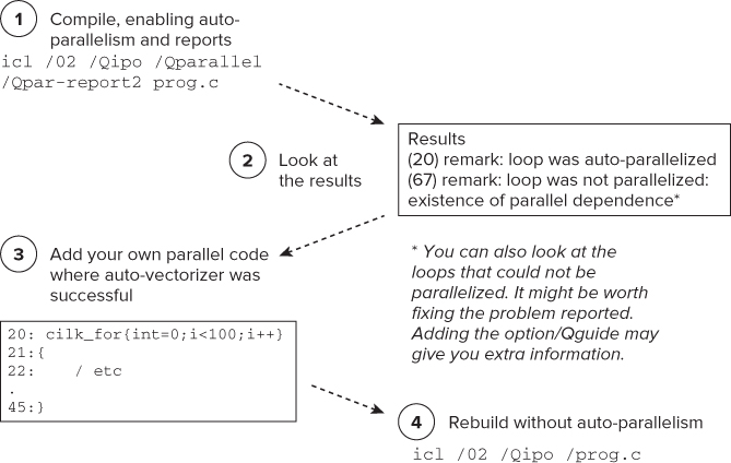
You might ask, “Why not just accept the results of the parallelizer?” The following are two of the common reasons:
- The auto-parallelizer (at the time of writing) uses OpenMP. Many developers prefer to use a more composable parallelism, such as that provided with Cilk Plus or Threading Building Blocks. In this context, “composability” refers to how well a parallel model can be mixed with other models.
- Some developers don't like relying on automatic features. They prefer to have more control over where and when threading is implemented.
An Example Session
Here's an example session of finding hotspots with the auto-parallelizer. You can try this out for yourself in Activity 6-3.
C: >serial.exe
calculating…
printing…
Time to calc :…3.667
Time to print :…2.311
Time (Total) :…5.978
icl /Zi /O2  wtime.c main.cpp  mandelbrot.cpp  ppm.cpp -o m1.exe
/Qparallel /Qipo /Qpar-report2
main.cpp(14):(col.3) remark: LOOP WAS AUTO-PARALLELIZED
main.cpp(14):(col.3) remark: loop was not parallelized: insufficient inner loop
main.cpp(14):(col.3) remark: loop was not parallelized: existence of parallel dependence
.
.
ppm.cpp(11):(col.3) remark: loop was not parallelized: existence of parallel dependence
ppm.cpp(12):(col.5) remark: loop was not parallelized: existence of parallel dependence
C:>parallel.exe
calculating…
printing…
Time to calc :…0.596
Time to print :…2.272
Time (Total) :…2.868
main.cpp 12: std::cout << "calculating…" << std::endl;
main.cpp 13:   double start = wtime();
main.cpp 14:   Mandelbrot();
main.cpp 15:   double mid = wtime();
mandelbrot.cpp 27:  void Mandelbrot ()
mandelbrot.cpp 28:  {
mandelbrot.cpp 29:    float xinc = (float)deltaX/(maxI-1);
mandelbrot.cpp 30:    float yinc = (float)deltaY/(maxJ-1);
mandelbrot.cpp 31:    for (int i=0; i<maxI; i++) {
mandelbrot.cpp 32:      for (int j=0; j<maxJ; j++) {
mandelbrot.cpp 33:      SetZ(i, j, xinc, yinc);
mandelbrot.cpp 34:      }
mandelbrot.cpp 35:    }
mandelbrot.cpp 36:  }
mandelbrot.cpp  0:  #include "mandelbrot.h"
mandelbrot.cpp  1:  #include <cilk/cilk.h>
mandelbrot.cpp 30:    float yinc = (float)deltaY/(maxJ-1);
mandelbrot.cpp 31:    cilk_for (int i=0; i<maxI; i++) {
mandelbrot.cpp 32:      for (int j=0; j<maxJ; j++) {
icl /Zi /O2  wtime.c main.cpp  mandelbrot.cpp  ppm.cpp -o myparallel.exe /Qipo

C:>myparallel.exe
calculating…
printing…
Time to calc :…0.2475
Time to print :…2.178
Time (Total) :…2.426
Programming Guidelines for Auto-Parallelism
Although this chapter is about using the auto-parallelizer to find hotspots, this is a good time to mention how you can help the auto-parallelizer to do its job better. For auto-parallelism to succeed, you must follow certain guidelines:
- The loop must be countable at compile time. Try to use constants where possible.
- There must be no data dependencies between loop iterations.
- Avoid placing structures in loop bodies (for example, function calls, pointers with ambiguous indirection to globals, and so on).
- Don't use the option /Od (or /Zi) on its own. Auto-parallelism will work only at optimization levels /O1 or greater.
- Use IPO (/Qipo). IPO gets applied before auto-parallelism and can improve the chance of the code being made parallel.
- Try to help the compiler by using the #pragma parallel option. (See the section “Using #pragma parallel.”)
Additional Options
Table 6.6 lists other options that you can use. Refer to the compiler help for more information.
Table 6.6 Some Auto-Parallelizer Options
| Option | Description |
| Qpar-affinity | Specifies thread affinity |
| Qpar-num-threads | Specifies the number of threads to use in a parallel region |
| Qpar-report | Controls the diagnostic information reported by the auto-parallelizer |
| Qpar-runtime-control | Generates code to perform runtime checks for loops that have symbolic loop bounds |
| Qpar-schedule | Specifies a scheduling algorithm or a tuning method for loop iterations |
| Qpar-threshold | Sets a threshold for the auto-parallelization of loops |
| Qparallel | Tells the auto-parallelizer to generate multithreaded code for loops that can be safely executed in parallel |
| Qparallel-source-info | Enables or disables source location emission when OpenMP or autoparallelization code is generated |
| Qpar-adjust-stack | Tells the compiler to generate code to adjust the stack size for a fiberbased main thread |
Helping the Compiler to Auto-Parallelize
To ensure correct code generation, the compiler treats any assumed dependencies as if they were proven dependencies, which prevents any auto-parallelization. The compiler will always assume a dependency where it cannot prove that it is not a dependency. However, if the programmer is certain that a loop can be safely auto-parallelized and any dependencies can be ignored, the compiler can be informed of this in several ways.
Using #pragma parallel
Used immediately before a loop, the #pragma parallel option instructs the compiler to ignore any assumed loop dependencies that would prevent correct auto-parallelization. It complements, but does not replace, the fully automatic approach; the loop will still not be parallelized if the compiler can prove that any dependencies exist.
Any loop being parallelized must conform to the for-loop style of an OpenMP work-sharing construct. The pragma can be used by itself or in conjunction with a selection of clauses, such as private, which acts in a similar way to the clauses used in the OpenMP method.
Currently, the clauses include the following:
- always[assert], which overrides the compiler heuristics that determine whether parallelizing a loop would increase performance. Using this clause forces the compiler to parallelize if it can, even if it considers that doing so might not improve performance. Adding assert causes the compiler to generate an error if it considers that the loop cannot be vectorized.
- private( var1[ :expr1][, var2[ :expr2] ] … ), where var is a scalar or array variable. When parallelizing a loop, private copies of each variable are created for each thread. expr is an optional expression used for array or pointer variables, which evaluates to an integer number giving the number of array elements. If expr is absent, the rules are the same as those used in the OpenMP method, and all the array elements are privatized. If expr is present, only that number of elements of the array are privatized. Multiple private clauses are merged as a union.
- lastprivate( var1[ :expr1][, var2[ :expr2] ] … ), where var and expr are the same as for private. Private copies of each variable are used within each thread created by the parallelization, as in the private clause; however, the values of the copies within the final iteration of the loop are copied back into the variables when the parallel region is left.
Following is an example of using #pragma parallel:
(41)    #pragma parallel private(b)
(42)    for( i=0; i<MAXIMUS; i++ )
(43)    {
(44)        if( a[i] > 0 )
(45)        {
(46)            b = a[i];
(47)            a[i] = 1.0/a[i];
(48)        }
(49)        if( a[i] > 1 )a[i] += b;
(50)    }
This results in the loop being both vectorized and parallelized, with the following messages:
C:Test.cpp(42): (col. 4) remark: LOOP WAS AUTO-PARALLELIZED.
C:Test.cpp(42): (col. 4) remark: LOOP WAS VECTORIZED.
Using #pragma noparallel
You can use the #pragma noparallel option immediately before a loop to stop it from being auto-parallelized.
Note that both #pragma parallel and #pragma noparallel are ignored unless the /Qparallel option is set.
- Pros
- Easy to carry out
- Quickly helps you spot the right places to parallelize
- Auto-parallelized loop can be compared with your own manually implemented parallelism
- Cons
- Can easily be confounded by nontrivial code
- Difficult to identify loops when IPO is enabled
icl /Zi /O2 /Qipo wtime.c main.cpp  mandelbrot.cpp  ppm.cpp -o 6-3.exe
   /Qparallel /Qpar-report2
speedup = new time / original time
#include <cilk/cilk.h>
.
.
 cilk_for (…etc ) {
.
.
.
icl /Zi /O2 /Qipo wtime.c main.cpp mandelbrot.cpp ppm.cpp -o 6-3b.exe
Instructions for Linux Users
Hotspot Analysis with Amplifier XE
The Hotspot analysis used in Amplifier XE helps you to identify the most time-consuming source code. Hotspot analysis also collects stack and call tree information. The analysis can be used to launch an application/process or attach to a running program/process.
Conducting a Default Analysis
The steps for conducting a Hotspot analysis with Amplifier XE were described in Chapter 3.
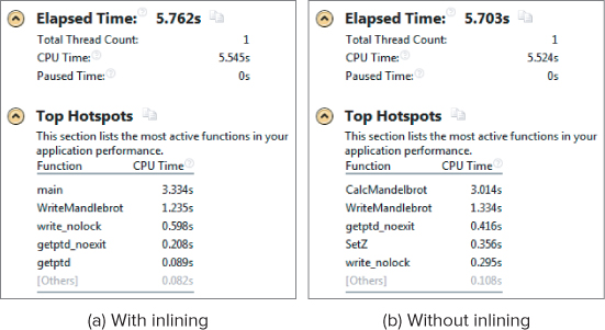
To get the best view of the application in Amplifier XE, it is best to disable inlining by using the /Ob0 or /Ob1 compiler options. The /Ob0 option disables all inlining, whereas the/Ob1 inlines only code that has been marked with the keywords inline, _inline_, _forceinline, _inline, or with a member function defined within a class declaration. (See online help for more information on these keywords.) Figure 6.5 shows the summary page of two Hotspot analysis sessions: one with inlining enabled (a) and one without (b). You can see that when inlining is disabled, the symbol names of the different functions become available.
Figure 6.5 Analysis summary with and without inlining
Finding the Right Loop to Parallelize
At the time of writing, Amplifier XE does not have a loop profiler, so you have to manually traverse up the call stack of a hotspot to find the best place to add parallelism. Figures 6.6 through 6.9 show screenshots of doing such a traversal. Clicking on the hotspot in Figure 6.6 displays the source view of the hotspot (Figure 6.7).
Figure 6.6 Bottom-up view of the hotspots
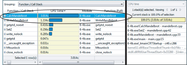
Figure 6.7 Source code view of the hotspots
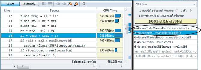
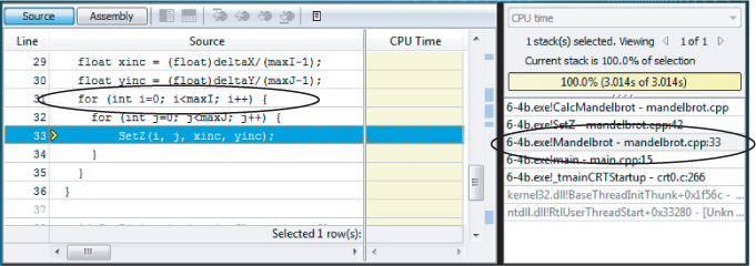
By double-clicking the stack pane on the right (see Figures 6.7 and 6.8), it is possible to traverse up the call stack until an appropriate place to add the parallelism is found, as in Figure 6.9.
icl /O2 /Qipo /Zi wtime.c main.cpp mandelbrot.cpp ppm.cpp -o 6-4.exe
amplxe-gui
Dealing with the Lack of Symbol Visibility
icl  /O2 /Qipo /Zi /Ob1 wtime.c main.cpp mandelbrot.cpp ppm.cpp
    -o 6-4.exe
Traversing Up the Call Stack
Instructions for Linux Users
Figure 6.8 Source code view, one stack up
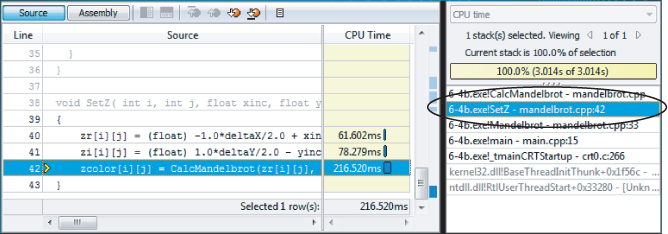
Figure 6.9 Source code view, two stacks up
Large or Long-Running Applications
In very large or long-running projects, the amount of data collected may grow to an unmanageable size. The postprocessing of the collected data (finalization) and opening and viewing very large data sets can become very sluggish and almost impractical to use.
Reducing the Size of Data Collected
Some strategies for reducing the amount of data collected include:
- Adjust the duration time estimate. Amplifier XE reduces the amount of samples it collects on very long runs. You can change the duration time estimate from “under 1 minute” to “over 3 hours,” with some intermediate values, as well.
- Automatically stop collection after a short period of time (for example, 30 seconds).
- Modify the data-collection limit. The default is 100MB.
- Use the Pause and Resume APIs to limit when data is collected.
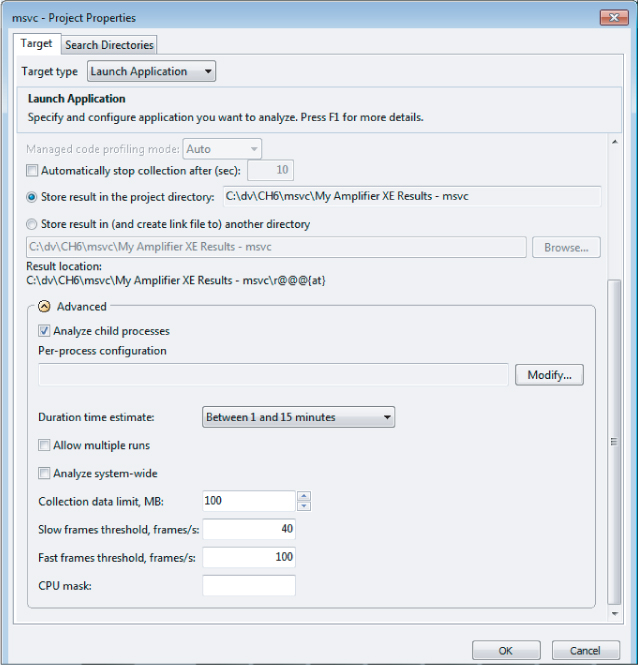
The first three items in the list are all configurable from the Project Properties dialog (see Figure 6.10), which you can access from the Amplifier XE menu File ⇒ Properties.
Figure 6.10 The Project Properties page
Using the Pause and Resume APIs
You can insert calls to the Pause and Resume APIs in your application to pause and resume data collection, respectively. By doing this you can reduce the amount of data that is collected. These APIs have to be used with caution, especially when analyzing threaded code, because important events may be missed, leading to a meaningless analysis.
The following code snippet shows how to use _itt_pause() and _itt_resume() functions in the Mandelbrot program:
#include "ittnotify.h"
.

int main()
{
  .
  .
  std::cout << "calculating…" << std::endl;
  double start = wtime();
  _itt_resume();
   Mandelbrot();
  double mid = wtime();

  std::cout << "printing…" << std::endl;
  WriteMandlebrot();
  _itt_pause();
  double end = wtime();
  .
  .
}
Once this code is inserted, any Hotspot analysis should be started by clicking the Start Paused button rather than the Start button.
To use the APIs, include the ittnotify.h header file. If you get an unresolved symbol at link time, you may have to add the libittnotify.lib library, which you can find in the Amplifier XElib32 or Amplifier XElib64 folders. Use the lib64 version if you are building a 64-bit application; otherwise, use the lib32 version.
Table 6.7 shows the difference in the size of data that is collected when doing a normal Hotspot analysis versus doing one with pauses and waits. As you can see, there is a significant saving in the amount of data collected.
Table 6.7 Amount of Data Collected when Profiling with and without the Pause and Resume APIs
| Method | Data Size |
| Without pause/resume | 253.9k |
| With pause/resume | 172.0k |
- Pros
- Very small profiling overhead
- Easy to traverse the call stack
- No special build needed, other than providing debug symbols
- Multiple options for collection and viewing
- Results can be compared
- Cons
- No loop profiler
- No call graph (but see the comments on manual call stack traversing in the section “Finding the Right Loop to Parallelize”)
Source Code
The source code in Listing 6.1 consists of several files and is used in the hands-on activities.
 Listing 6.1: main.cpp
main.cpp
#include <fstream>
#include <iostream>
#include <iomanip>
#include "mandelbrot.h"

float zr[maxI][maxJ],zi[maxI][maxJ];
float zcolor[maxI][maxJ];
extern "C" double wtime();

int main()
{
  std::cout << "calculating…" << std::endl;
  double start = wtime();
  Mandelbrot();
  double mid = wtime();

  std::cout << "printing…" << std::endl;
  WriteMandlebrot();
  double end = wtime();

  std::cout << "Time to calc :…"<< std::setprecision(4)
     << mid-start <<std::endl;
  std::cout << "Time to print :…" << end-mid <<std::endl;
  std::cout << "Time (Total) :…" << end-start <<std::endl;
}
code snippet Chapter6main.cpp
MANDELBROT.CPP
#include "mandelbrot.h"

float CalcMandelbrot(float r,float  i)
{
  float zi = 0.0;
  float zr = 0.0;

  int itercount = 0;

  float maxit = (float)maxIteration;
  while(1) {
  itercount++;
  float temp = zr * zi;
  float zr2 = zr * zr;
  float zi2 = zi * zi;
  zr = zr2 - zi2 + r;
  zi = temp + temp + i;
  if (zi2 + zr2 > maxThreshold)
    return (float)256*itercount/maxit;
  if (itercount > maxIteration)
    return (float)1.0;
  }
  return 1;
}

void SetZ( int i, int j, float xinc, float yinc )
{
  zr[i][j] = (float) -1.0*deltaX/2.0 + xinc * i;
  zi[i][j] = (float) 1.0*deltaY/2.0 - yinc * j;
  zcolor[i][j] = CalcMandelbrot(zr[i][j], zi[i][j] ) /1.0001;
}

void Mandelbrot ()
{
  float xinc = (float)deltaX/(maxI-1);
  float yinc = (float)deltaY/(maxJ-1);
  for (int i=0; i<maxI; i++) {
    for (int j=0; j<maxJ; j++) {
      SetZ(i, j, xinc, yinc);
    }
  }
}
code snippet Chapter6mandelbrot.cpp
MANDELBROT.H
#ifndef _MANDLE_H_
#define _MANDLE_H_
const int factor = 8;
const int  maxThreshold = 96;
const int  maxIteration = 500;
const int maxI = 1024 * factor;
const int  maxJ = 1024 * factor;
const float deltaX = 4.0;
const float deltaY = 4.0;

extern float zr[maxI][maxJ],zi[maxI][maxJ];
extern float zcolor[maxI][maxJ];

void Mandelbrot ();
void WriteMandlebrot();
#endif
code snippet Chapter6mandelbrot.h
PPM.CPP
#include <fstream>
#include "mandelbrot.h"

// write to a PPM file.
void WriteMandlebrot()
{
  std::ofstream ppm_file("default.ppm");
  ppm_file << "P6 " << maxI << " " << maxJ << " 255" << std::endl;

  unsigned char red, green, blue; // BLUE - did minimal work
  for (int i=0; i<maxI; i++) {
    for (int j=0; j<maxJ; j++) {
      float color = (float)zcolor[i][j] ;
      float temp = color;
      if (color >= .99999)
      {
        red = 255 ; green = 255; blue = 255;
      }
      else
      {
        red = 0 ; green = 0; blue = 0;
      }
      // write to PPM file
      ppm_file << red  << green << blue;
    }
  }
}
code snippet Chapter6ppm.cpp
WTIME.C
#ifdef _WIN32
#include <windows.h>
double wtime()
{
  LARGE_INTEGER ticks;
  LARGE_INTEGER frequency;
  QueryPerformanceCounter(&ticks);
  QueryPerformanceFrequency(&frequency);
  return (double)(ticks.QuadPart/(double)frequency.QuadPart);
}
#else
#include <sys/time.h>
#include <sys/resource.h>
double wtime()
{
  struct timeval time;
  struct timezone zone;
  gettimeofday(&time, &zone);
  return time.tv_sec + time.tv_usec*1e-6;
}
#endif
code snippet Chapter6wtime.c
Summary
This chapter described several methods of finding hotspots within an application. In practice you would probably want to use a combination of the methods to get best results. The identification of the hotspots is essential if you want to avoid wasted effort in attempting parallelism of any existing code.
It is very easy to apply parallelism at every opportunity you see within the code — for example, at every loop. However, many of these loops may not be invoked often enough nor do enough work, to make the effort of their parallelism worthwhile. Some loops that are tempting to parallelize may not really contribute much to the overall run time.
Finding the parallelization opportunities within your code is the goal of Hotspot analysis. It is an essential first step in adding parallelism to your code. Without this knowledge of your program, you are in danger of making code parallel without seeing any improvement in performance.
Having found the hotspots, the next steps are to implement the parallelism, check for errors, and, finally, tune the threaded application. The next chapter shows how to use different programming models to implement parallelism.