
CHAPTER 9
How to Assess Risk
The Difference Between Risk and Uncertainty
On Wall Street, risk and uncertainty are often used interchangeably, although, as we discuss below, they are not the same thing. That fact is apparent if one simply looks at the definition of each term in the Merriam-Webster dictionary:
- Uncertainty: Something that is doubtful or unknown
- Risk: Possibility of loss or injury
We illustrate the difference with a simple story:
Your grandmother gives you a lottery ticket as a birthday present.1 It is impossible to know if the ticket is a winner before the lottery is held. There is uncertainty to the outcome, but no risk because you have nothing to lose.
Next, assume that you buy a $2 ticket for the same lottery. In this case, there is uncertainty AND risk. The uncertainty is the same as with the ticket your grandmother gave you, but there is now the possibility of losing the $2 you paid for the ticket. The lottery ticket you purchased has financial risk because of the very real possibility of losing money.
As the example demonstrates, because uncertainty has no harm associated with it, there is no risk. It is only when an investor commits capital to an uncertain outcome that he is exposed to risk.
Merriam-Webster defines uncertainty as “something that is doubtful or unknown.” It is critically important to note that uncertainty is not necessarily bad and in many situations can be good.2 In general, however, humans crave certainty and hate uncertainty. Certainty makes us feel safe and secure, informed and intelligent, and in control, while uncertainty makes us feel insecure, in doubt, and powerless, and, in turn, often triggers fear. What are we afraid of? We fear the possibility of loss or injury, which is why most individuals equate uncertainty with risk.

Confusing Uncertainty and Risk Causes Mispricings
Confusing uncertainty with risk is a common investor mistake. For instance, most investors will avoid investment opportunities with a high degree of uncertainty, even if the potential return is high and the actual risk is low, because they (as human beings) hate uncertainty. Investors often process these opportunities incorrectly because they confuse uncertainty for risk and price the security accordingly. Shrewd investors, on the other hand, view these types of situations as opportunities because the actual risk is mispriced by the consensus.
In an interview in Graham & Doddsville, Dan Krueger, a portfolio manager at Owl Creek Asset Management responsible for the Herbalife bond analysis we discuss in the previous chapter, explained his views on the difference between risk and uncertainty while analyzing Lehman Brothers bonds during the 2008 Financial Crisis:
Uncertainty, to us as distressed investors, is our friend, because uncertainty is something investors will pay to avoid—sometimes pay a large amount. We love situations like Lehman which we call “high uncertainty, low risk.”3
Krueger explained further that there was a lot of uncertainty surrounding the Lehman bonds because of the “hundreds of unanswered questions,” which he knew “would eventually get answered over the coming months, quarters or years.” He added that “occasionally you’ll be given an opportunity to buy something at a price where even though you have a hundred unanswered questions, you realize that regardless of what the answers are, you probably cannot lose a lot of money, and most of the time you will make a little or a lot.” Exploiting other investors’ confusion of risk and uncertainty can be highly profitable and is one of the key reasons we feel the need to distinguish between the two concepts.
How Confusion of Risk and Uncertainty Manifests in the Wisdom of Crowds Framework
When investors confuse uncertainty for risk, that mistake shows up primarily as a processing error, which produces a systematic bias in the wisdom of crowds framework, as shown in Figure 9.1.

Figure 9.1 Consensus Decision Model Distorted by Error in Processing
As we discuss in the Sevcon example in Chapter 7, the crowd’s diversity collapsed when investors panicked in response to Sevcon losing its biggest customer and all the investors began using the same liquidation model to estimate the company’s intrinsic value.
Similarly, as we explain in Chapter 8, Bill Ackman caused a breakdown of independence in the consensus view concerning the outlook for Herbalife’s bonds because of the high degree of uncertainty his presentation created. Many of the investors misinterpreted the perceived uncertainty as a risk of potential capital loss, which caused a mispricing in the bonds that Dan Krueger and other shrewd investors were able to exploit.
When Uncertainty Becomes Risk
When does uncertainty become risk? As we discuss at the beginning of the chapter, risk becomes a factor only when capital is committed, and therefore is always a function of the price paid for the investment.
We show Tesla’s stock price relative to the consensus estimate for the company’s one-year price target and each individual analyst’s estimates in Chapter 4, which we replicate in Figure 9.2.

Figure 9.2 Tesla: Analysts’ One-Year Price Targets
We removed the individual analyst estimate in Figure 9.3 so that we can present an uncluttered distribution of estimates.

Figure 9.3 Tesla: Consensus Estimate
The difference between the market price of $245 and the consensus one-year price target of $293 is the stock’s expected return, which equals 19.6% in the example, as shown in Figure 9.4.

Figure 9.4 Tesla: Expected Return Implied by Consensus Price Target
It is straightforward to see from the distribution in Figure 9.5 that the investment will lose money if the actual intrinsic value turns out to be less than the price paid for the stock. In Figure 9.5, all possible outcomes less than the market price are depicted by the red-shaded area in the chart and represent the market implied risk of investing in the stock.

Figure 9.5 Tesla: Market Implied Risk of Investing in Stock at $245 per Share
While all possible outcomes above the stock price are also uncertain, there is no risk because these outcomes will not result in a loss of capital. The uncertainty is represented by the sky blue-shaded area in Figure 9.6 and illustrates the difference between risk and uncertainty.

Figure 9.6 Tesla: Outcomes Above Market Price are Uncertain But Not Risky
It should be clear from this discussion that the level of risk will change when the market price changes if the range of expected intrinsic values remains the same. To illustrate this point, we start with the initial assumptions presented in Figure 9.7. If the stock price increases from $245 to $278, as shown in Figure 9.8, with no change in the estimated intrinsic value, the expected return declines (falling from 19.6% to 5.4% in the example) and risk increases substantially, as we show in Figure 9.9.

Figure 9.7 Tesla: Initial Expected Return versus Market Implied Risk

Figure 9.8 Tesla: Stock Price Increase from $245 to $278

Figure 9.9 Tesla: Increase in Price Results in Lower Expected Return and Additional Risk
The reverse is also true. If the market price declines from $278 to $245, without any change in the range of estimated intrinsic values, the potential return increases while the risk is reduced, as depicted by the charts in Figures 9.10, 9.11, and 9.12.

Figure 9.10 Tesla: Market Implied Risk with Stock Price of $278

Figure 9.11 Tesla: Stock Price Declines from $278 to $245

Figure 9.12 Tesla: Lower Price Produces Higher Expected Return and Lower Market Implied Risk
We define risk as the possibility of a loss of capital, which is equivalent to the possibility of losing money. Therefore, although the future is inherently uncertain, there is no risk until capital is committed, as the examples show, and the level of risk will be a direct function of the price paid relative to all possible outcomes.

Margin of Safety Is Really All about Risk
Ben Graham devoted an entire chapter to the discussion of risk in The Intelligent Investor, in which he distilled to “the secret of sound investment into three words . . . MARGIN OF SAFETY.” Graham’s concept of risk is fully captured by his definition of margin of safety, which he describes as:
A favorable difference between price on the one hand and indicated or appraised value on the other. That difference is the safety margin. It is available for absorbing the effect of miscalculations or worse than average luck. The buyer of bargain issues places particular emphasis on the ability of the investment to withstand adverse developments.5
It is straightforward to show that the area between the stock’s price and the intrinsic value (Graham’s “appraised value”), represents what is generally accepted as the investment’s margin of safety, as shown in Figure 9.13.

Figure 9.13 Margin of Safety Equals Expected Return
Mirroring our previous discussion, Graham adds, “The margin of safety is always dependent on the price paid. It will be large at one price, small at some higher price, nonexistent at some still higher price.”6
A More Certain Business Can Actually Be Riskier
As we discuss in Chapter 4, the distribution of the estimates of intrinsic value will be narrower when the company’s cash flows are more predictable. Likewise, the distribution of the estimates of intrinsic value will be wider when the cash flows are less certain. We illustrated this point by comparing analysts’ one-year price targets for Tesla with McCormick’s, as shown in Figure 9.14.

Figure 9.14 McCormick and Tesla Consensus Estimates of One-Year Price Targets
At the time we originally performed this analysis, McCormick’s stock price was $85, which was above the consensus estimated one-year price target of $79. Ironically, while McCormick’s future cash flows were highly predictable and more certain than Tesla’s, if analyst forecasts at that time were correct, then McCormick stock was riskier because it had no margin of safety, as shown in Figure 9.15.
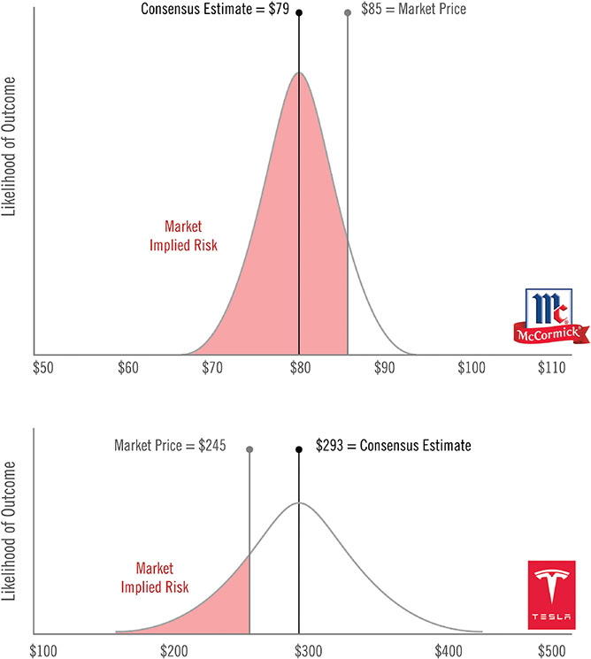
Figure 9.15 Comparing the Risk of McCormick and Tesla

Time Matters . . . and Matters a Lot . . .
In addition to the risk of capital loss, portfolio managers also face the risk of underperforming their benchmark. It continually surprises us that most of the portfolio managers, analysts, and institutional salespeople we have observed in our careers spend almost all their time concerned with estimating the company’s intrinsic value and little time estimating the investment’s time horizon. We think this time allocation is a critical mistake because time is a key component in the ultimate return the investment delivers.
Therefore, before discussing the risks from errors in estimating the investment’s time horizon, we want to make sure the reader fully understands why time is such a critical element in the investment return.
The return from investing in a stock, or any security for that matter, is determined by three elements: the price you pay, the value you get, and the time it takes for the investment to work out, and is calculated using the following formula.
![Diagram shows rate of return equals [(what you receive/your cash outlay)how long it takes] minus 1.](http://images-20200215.ebookreading.net/13/1/1/9781119051787/9781119051787__pitch-the-perfect__9781119051787__images__c09uf006.jpg)
We need to change the labels slightly to account for the fact that we are evaluating a potential investment, one that we have not yet made. Since we do not know for certain what will happen in the future, or how much we will earn from the investment, we relabel what we get as estimated value, while what we pay becomes current market price and time becomes expected time horizon.

We use the stock of ZRS Corporation as a simple example to demonstrate how to calculate the expected rate of return for a stock. The company’s stock trades at $5.85 per share and we estimate it will be worth $10.25 per share within four years. The expected annualized rate of return is 15.0%, as the following calculation shows.

Of the three inputs in the expected rate of return formula, the current market price is the only input that is known ahead of time, which is the price you would pay to purchase the stock and can be easily determined by looking at the stock’s market price. The other two inputs, the estimated value and expected time horizon, are estimates, which we show graphically in Figure 9.16.

Figure 9.16 Three Components of Investment Return
We use the return formula to calculate an expected rate of return of 15.0% based on the initial market price of $5.85, the estimated ending value of $10.25, and a time horizon of four years. We show the convergence of these three factors, and the expected return, in Figure 9.17.

Figure 9.17 Expected Rate of Return
What if we are wrong? The primary assumption behind every investment is that the current market price will converge to the estimated value within the expected time horizon. However, if the estimated value is wrong or if it takes longer than we expect for the stock to close the gap between price and value, then the actual return will be less than what we have forecast.
For instance, if we are right on the expected value of $10.25, but it takes the stock seven years, instead of four years, to reach that price, then the return falls almost in half to 8.3% per year, as shown in Figure 9.18.

Figure 9.18 Error in Estimating Time Horizon
This example highlights that time is a critical factor in the ultimate return the investment delivers. On the other hand, if we are right in the estimate of the time horizon, but wrong about the expected value for ZRS stock, such that it is worth only $7.00 in four years, then the return falls to 4.6% per year, as shown in Figure 9.19.

Figure 9.19 Error in Estimating Intrinsic Value
Now that we have presented a comprehensive understanding of the components of return and the importance of time as a factor in that return, we can discuss how increased accuracy and precision in estimating both the intrinsic value and time horizon can reduce risk significantly.
How Increased Accuracy and Precision in Estimating Intrinsic Value Affects Risk
As we discuss in the previous chapter, investors perform research to improve the accuracy and precision of their estimate of a company’s intrinsic value with the goal of producing as tight a range of estimated intrinsic values as possible.
Figure 9.20 shows the difference between accuracy and precision. The targets were shot at 200 yards with a bolt action Eliseo RTS Tubegun chambered in a 6.5 x 47 Lapua. The center of the black box is the actual target—not the bullseye—as mirage makes it difficult to see the rings of a typical target at 200 yards.10 At this distance, a group of one-half inch is considered very precise.

Figure 9.20 The Difference Between Accuracy and Precision
Low accuracy and low precision are obviously not the goal in this exercise. High precision with low accuracy is even worse as you will completely miss the target. High accuracy with low precision is better, although high accuracy and high precision is ideal.
We show in the first example how increased accuracy reduces risk. We start with the initial assumptions that the stock trades at $80, the consensus estimate of the intrinsic value is $85, and the true intrinsic value is $95, as shown in Figure 9.21.

Figure 9.21 Initial Assumptions
After completing your research, you estimate that the intrinsic value per share is $90. Assuming you are correct, your estimate is more accurate than the consensus because it is closer to the true intrinsic value of $95. In Figure 9.22, the green-shaded area shows your increased accuracy and the red-shaded area shows the new implied estimate of risk.

Figure 9.22 Research Results in Greater Accuracy
As a result of the greater accuracy in your estimate, the implied level of risk has been reduced, as shown in Figure 9.23.

Figure 9.23 Increased Accuracy Reduces Risk
We use the same initial assumptions in the next example to demonstrate how risk is reduced by increasing the precision of your estimate of intrinsic value, as shown in Figures 9.24, 9.25, and 9.26.
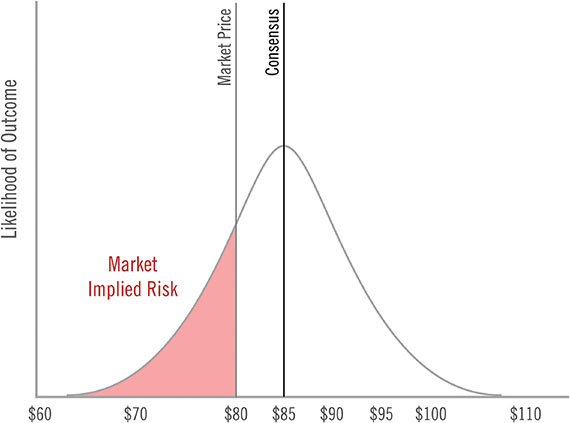
Figure 9.24 Initial Assumptions

Figure 9.25 Your Estimate of Risk
Figure 9.25 shows how risk is reduced with greater precision:

Figure 9.26 Greater Precision Reduces Risk
After completing your research (assuming you are correct), you arrive at a more precise estimate than the consensus, thereby reducing the uncertainty, which reduces the implied level of risk of the investment, as shown in Figure 9.25.
Figure 9.26 shows how risk is reduced with greater precision:
As we have just demonstrated, increased accuracy and increased precision individually reduce risk. However, risk is reduced even more significantly when both accuracy and precision are combined. We use the same initial assumptions as in the previous two examples to make the point, as shown in Figure 9.27.

Figure 9.27 Initial Assumptions
Because of your increased accuracy and precision there will be an extremely low level of risk (assuming you are correct), as shown in Figure 9.28:

Figure 9.28 Increased Accuracy and Precision Reduce Risk Significantly
Figure 9.29 shows the reduction in risk as the result of increased accuracy and precision.

Figure 9.29 Risk Reduction from Initial Condition
How Increased Accuracy and Precision in Estimating Time Horizon Affects Risk
It is not enough for the estimate of intrinsic value to be correct; the investor also must be accurate in his estimate of the amount of time it takes to close the gap between market price and intrinsic value because the actual time horizon will determine the realized annual return.
Just as it is important to recognize that there is a range of possible outcomes for intrinsic value, it is helpful to think of the expected time horizon as a range of outcomes rather than a single-point estimate, as shown in Figure 9.30.

Figure 9.30 Range of Estimated Time Horizon
The red-shaded area in Figure 9.31 shows the implied risk from errors in underestimating the time horizon.

Figure 9.31 Implied Risk in Estimated Time Horizon
Errors in underestimating the time horizon of an investment are a source of risk because any error reduces the realized investment return, as we show in Figure 9.18 and replicate below.

Figure 9.32 Figure 9.18: replicated
Risk and Variant Perception—Skewing the Distribution in the Investor’s Favor
For simplicity, many of the figures in this chapter present the range of possible intrinsic values as a normal distribution around a single-point estimate. The normal distribution was a useful fiction to highlight the relationship between price and intrinsic value, as well as demonstrate how the price paid determines the level of risk. However, it is important to note that an investor will rarely be able to determine a precise probability for each estimate of intrinsic value, therefore, it will be difficult to ever know the actual shape of the distribution of possible values.
Nonetheless, we can use the following example to show how an investor can perform research to skew the distribution of intrinsic value estimates in his favor and reduce the risk of the investment as a result. We begin with a normal distribution in Figure 9.33 to represent the range of possible intrinsic values, a market price of $70, and a consensus estimate of intrinsic value of $75. The area to the left of the market price represents the market implied risk in the investment, as we discuss in previous examples.

Figure 9.33 Market-implied Risk
Now suppose the investor performs extensive research, develops a variant perspective, and determines that there is less downside to the investment than implied by the consensus view. His distribution of possible intrinsic values will be skewed to the upside, as shown in Figure 9.34:
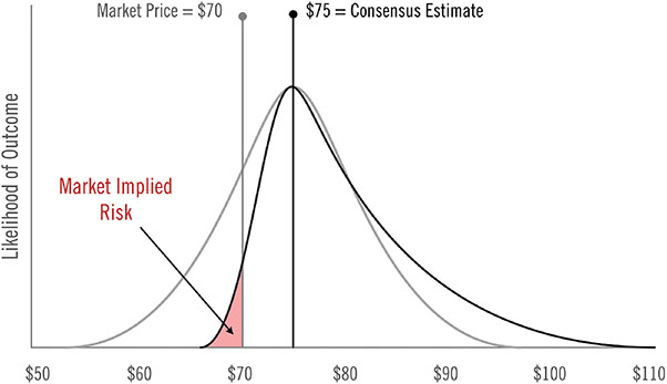
Figure 9.34 Normal Versus Skewed Distribution
Figure 9.35 shows that the skewed distribution significantly reduces the market implied level of risk in the investment.

Figure 9.35 Risk Reduction Due to Skewed Distribution
Investments with skewed distributions have asymmetric returns. Positively skewed distribution have more upside than downside, which maximizes the upside potential of the investment and minimizes its implied risk, while negatively skewed distributions have more downside than upside. Shrewd, experienced investors are always on the hunt for investment opportunities with positively skewed distributions.
For instance, rather than a normal distribution, the range of consensus expectations for Cloverland’s intrinsic value, which we discuss in Chapter 8, is negatively skewed, as we show in Figure 9.36. The analysis highlights the relationship between the market price of $85, the estimated intrinsic value of $107, and the implied risk of capital loss as the red shaded area to the left of the price. Because timber is a hard asset, most investors assume that its value will not change much over time and, therefore, there will be minimal upside potential to Cloverland’s appraised value of $107, as the chart shows. On the other hand, there are various scenarios that can produce a lower intrinsic value, such as corporate mismanagement, the continued under-cutting of trees, or some type of infestation that destroys the health of a large portion of the timberlands.

Figure 9.36 Consensus Implied Risk For Cloverland
As we discuss in Chapter 8, John Helve of Brownfield Capital has a variant perspective concerning the company and his distribution curve of possible intrinsic values that looks significantly different than the consensus view, as shown in Figure 9.37. Although Helve recognizes that there is the possibility of a loss with his investment, he estimates the probability of that risk as being low, as the chart shows. If Helve is successful in forcing a sale of the company, which he believes is highly probable, his estimated intrinsic value would equal $142, with only a small probability of it being worth significantly less than this estimate, as the chart shows. It should be noted that because of his variant perspective, Helve does not believe there is a scenario where he would lose money, therefore, in his view, there is no risk to the investment.

Figure 9.37 Helve’s Variant Perspective Results in Lower Risk
The Risk of Underperforming
We have limited the discussion of risk so far to the potential of a capital loss (losing money), which we show as negative returns in Figure 9.38.

Figure 9.38 Heat Map: Risk of Capital Loss
However, a return of zero is not the appropriate benchmark to use when evaluating a portfolio manager’s investment results for the simple reason that all capital has an opportunity cost, as we discuss in Chapter 2. The performance of most professional portfolio managers is benchmarked against an index such as the S&P 500 or Russell 2000. Consequently, underperforming the market is a legitimate concern for most professional portfolio managers because investors have a viable alternative (investing in the index) and will redeem their investment if the manager underperforms the market.
Returning to the Cloverland example, Helve is sensitive to his investment underperforming the market for the reasons just listed. As a result, his variant perspective regarding the estimated time horizon is a critical factor in his investment thesis, which we show is significantly different than consensus expectations in Figure 9.39.

Figure 9.39 Helve’s Variant Perspective Regarding Time Horizon
And, as we show in Figure 9.40, Cloverland’s stock will outperform the market if the sale of the company takes place in less than five years, which is Helve’s belief, but will underperform if the transaction takes longer to occur, which is the consensus view. Helve knows that getting the timing right is critical to his investment because of the ever-present need to outperform the market.

Figure 9.40 Cloverland: Break-even Investment Time Horizon
While most professional portfolio managers are keenly aware that their performance will be benchmarked against the market, others successful investors view the concern as less important. For instance, in 1984, on the television show Adam Smith’s Money World, Warren Buffett made a statement that over time has morphed into the quote, “There are no-called-strikes in investing,” referring to the fact that he believes missed opportunities are not harmful and an investor should not feel undue pressure to invest if they fail to find opportunities that meet their investment criteria. However, as Columbia Professor Bruce Greenwald wryly counters, in professional money management, because there is always the option of investing in an index fund, “they keep running up the score while you wait for the perfect pitch.” For this reason, relative performance matters for most professional portfolio managers.11 This discussion emphasizes that there are two risks to any investment opportunity—the risk of capital loss and the risk of underperformance, as we show in the heat maps in Figures 9.38 and 9.41.

Figure 9.41 Heat Map: Risk of Underperformance
Gems:
- Uncertainty has no harm associated with it and, therefore, entails no risk. It is only when an investor commits capital to an uncertain outcome that he exposes himself to risk. In general, humans crave certainty and hate uncertainty. Certainty makes us feel safe and secure, informed and intelligent, and in control, while uncertainty makes us feel insecure, in doubt, and powerless, and, in turn, often triggers fear. What are we afraid of? We fear the possibility of loss or injury, which is why individuals often equate uncertainty with risk.
- The most commonly-recognized risk of any investment is the possibility that the actual intrinsic value will be less than the price paid for the investment (or stock), which will result in permanent loss of capital. If the intrinsic value remains constant, an increase in price creates a lower expected return and higher risk, while a lower price creates a higher expected return and lower risk. Market price and risk are positively correlated—the higher the price paid, the higher the risk.
- Uncertainty and risk are not synonymous. Less uncertainty does not automatically mean less risk. In fact, stocks for companies with more certain cash flows can be riskier than companies with less certain cash flows because the level of risk is a function of the price paid and not the uncertainty in the situation.
- Increased accuracy and increased precision both reduce risk. However, the estimated level of risk is reduced even more significantly when both improvements are combined.
- Time is a critical factor in the investment’s actual realized rate of return and, as a consequence, an additional source of risk. In other words, it is not enough to be correct about a company’s true intrinsic value; the investor also must be accurate in his estimate of the amount of time it takes to close the gap between market price and intrinsic value because the actual time horizon will determine the realized annual return.
- A return of zero is not the appropriate benchmark to use when evaluating a portfolio manager’s investment results for the simple reason that all capital has an opportunity cost. Most professional portfolio managers’ performance is benchmarked against an index such as the S&P 500 or Russell 2000 for this very reason, and underperforming the market is a legitimate concern because investors have a viable alternative and will redeem if the manager underperforms the market consistently.
- A portfolio manager faces two risks to any investment opportunity—the risk of capital loss and the risk of underperformance.