
Optimal Placement and Sizing of Shunt Capacitor Banks in the Presence of Harmonics
Abstract
Investigates the optimal placement and sizing of shunt capacitor banks in the presence of harmonics. It includes the concept of reactive power compensation based on capacitors, and common types of shunt capacitor banks used in power systems. A survey of various optimization algorithms for the placement and sizing of shunt capacitor banks under sinusoidal operating conditions is listed, such as analytical methods, numerical programming methods, heuristic methods, artificial intelligence-based methods, genetic algorithms, expert systems, simulated annealing, artificial neural networks, fuzzy set theory, graph search algorithm, particle swarm algorithm, tabu search algorithm, and sequential quadratic programming. The analysis and comparison of various solution approaches for the optimal placement and sizing of fixed capacitor banks in the presence of voltage and current harmonics are outlined. This chapter includes 8 application examples with solutions.
At the distribution level about 13% of the total generated power consists of losses due to active and reactive current components. Research over the past several decades has shown that proper placement of shunt-capacitor banks can reduce the losses caused by reactive currents [1–34]. In addition to the reduction of energy and peak-power losses, effective capacitor installation can also release additional reactive power capacity within the distribution system and can improve the system voltage profile. Studies [35–46] indicate that the proper placement of shunt capacitors in the presence of voltage and current harmonics can also improve power quality and reduce the total voltage harmonic distortion (THDv) of distribution systems. Thus, the problem of capacitor allocation involves the determination of the optimal locations, sizes, and number of capacitors to be installed within a distribution system such that maximum benefits are achieved, while all operational constraints (e.g., voltage profile, THDv, and total number of capacitor banks at each bus and the entire system) are satisfied at different loading levels. There are a great many papers describing capacitor placement algorithms: the Capacitor Subcommittee of the IEEE Transmission and Distribution Committee has published 10 bibliographies on power capacitors from 1950 to 1980 [33]. Moreover, the VAr Management Working Group of the IEEE System Control Subcommittee has published another bibliography on reactive power and voltage control [34]. The total publication count listed in these bibliographies is over 400, and many of the papers are specific to the problem of optimal capacitor allocation [1–46]. Recent efforts mainly focus on the capacitor placement under nonsinusoidal operating conditions.
In power systems, the predominantly inductive nature of loads and distribution feeders as well as transformers and lines accounts for significant power losses due to lagging currents. The introduction of strategically sized and placed shunt capacitors within the distribution system helps to reduce the losses created by an inductive system, thus increasing the system capacity, reducing system losses, and improving the voltage profile. Due to the fact that there are many constraints and variables present, the process for calculating the placement and sizing of shunt capacitors involves the evaluation of an optimization function. Often this function will not only address technical aspects of a problem, but will evaluate its cost as well. Therefore, it becomes necessary to design an approach that will optimize the solution at minimal cost.
Analyses of this chapter are restricted to the application of shunt capacitor banks for reactive power compensation of distribution systems under sinusoidal as well as nonsinusoidal operating conditions. The capacitor placement problem of a distribution system consists of determining the optimal locations, sizes, and types of capacitor banks in order to achieve maximum annual benefits within the permissible region of constraints (e.g., bus voltage deviation, total harmonic distortion, number of capacitor banks at each bus and the entire system). Various techniques and algorithms have been proposed and implemented for solving this problem under normal sinusoidal conditions and in the presence of voltage and current harmonics. All such methods have their own advantages, disadvantages, and limitations as stated by their assumptions.
The goal of this chapter is to show the progression of research in optimal capacitor placement for sinusoidal operating conditions and to introduce a number of algorithms for solving this problem in the presence of harmonics. Section 10.1 presents the concept of reactive power compensation based on capacitors. Section 10.2 addresses common types of shunt capacitor banks as used in power systems. A survey of various optimization algorithms for the placement and sizing of shunt capacitor banks under sinusoidal operating conditions is presented in Section 10.3. The last part of the chapter includes analysis and comparison of various solution approaches for the optimal placement and sizing of fixed capacitor banks in the presence of voltage and current harmonics.
10.1 Reactive power compensation
Reactive power compensation is an important issue in electric power systems involving operational, economic, and quality of service aspects. Consumer loads (residential, commercial, industrial, service sector, etc.) impose active and reactive power demands. Active power is converted into useful energy, such as light, heat, and rotary motion. Reactive power must be compensated to guarantee an efficient delivery of active power to loads.
Capacitor banks are widely employed in distribution systems for reactive power compensation in order to achieve power and energy loss reduction, system capacity release, and acceptable voltage profiles. The extent of these benefits depends on the location, size, type, and number of shunt capacitors (sources of reactive power) and also on their control settings. Hence an optimal solution for placement and sizing of shunt capacitors in a distribution system is a very important aspect of power system analysis.
10.1.1 Benefits of Reactive Power Compensation
Shunt capacitors applied at the receiving end of a power system feeder supplying a load at lagging power factor have several benefits, which may be the reason for their extensive applications. This section highlights some advantages of reactive power compensation.
Improved Voltage Profile
Highly utilized feeders with high reactive power demands have poor voltage profiles and experience large voltage variations when loading levels change significantly. In a power system, it is desirable to regulate bus voltages within a narrow range (e.g., + 5%, –8% of their nominal values) and to have a balanced load on all three phases (eliminating negative- and zero-sequence currents with undesirable consequences such as equipment heating and torque pulsations in generators and turbines). However, loads of the power system fluctuate and can result in voltage deviations beyond their acceptable limits. In view of the fact that the internal impedance of the AC system is mainly inductive, it is the reactive power change of the load that has the most adverse effect on voltage regulation.
Traditionally, line voltage drop is compensated with distributed capacitors along a feeder, and by switching them according to the reactive power demand a rather constant voltage profile is achieved. Furthermore, by keeping the power factor close to unity along the section in question, the number of expensive voltage regulators can be minimized.
Impacts of active and reactive current variations on the terminal load voltage (Vt) are demonstrated in Fig. 10.1. An increase of ΔQ in the lagging VArs drawn by the load (indicated by quantities with primes in Fig. 10.1b) causes the reactive current component to increase to (Iq + ΔIq) while the active current component Ip is assumed to be unchanged. This will result in a terminal voltage drop of ΔVt and decreases the real power. Figure 10.1c shows the phasor diagram where the active current component increases to (Ip + ΔIp) with ΔIp = ΔIq (of Fig. 10.1b) while Iq is assumed to be unchanged. Comparison of phasor diagrams indicates that variations in reactive power (Fig. 10.1b) have more impact on voltage regulation as compared with active power variations (Fig. 10.1c).

Reduced Power System Losses
Correcting the power factor can substantially reduce network losses in between the point in the network where the correction is performed and the source of generation. This can result in an annual gross return of as much as 15% on the capacitor investment [48]. To maximize benefits, power factor correction should be implemented as close to the customer load as possible. However, due to economies of scale, installation of capacitors at the low-voltage (LV) level is very costly when compared with high-voltage (HV) options.
In most industrial plant power distribution systems, the I2R losses vary from 2.5 to 7.5% of the load kWh. This depends on the hours of full-load and no-load plant operation, wire size, and length of the main and branch feeder circuits. Capacitors are effective in reducing only that portion of the losses that is due to the reactive current. Losses are proportional to the current squared, and since current is reduced in direct proportion to power factor improvement, the losses are inversely proportional to the square of the power factor. Hence, as the power factor is increased with the addition of capacitor banks to the system, the amount of the losses is reduced. The connected capacitor banks have losses, but they are relatively small. Losses account for approximately one-third of one percent of the reactive power rating [48].
Released Power System Capacity
When capacitors are placed in a power system, they deliver reactive power and furnish magnetizing current for motors, transformers, and other electromagnetic devices. This increases the power factor and it means that for a lower current (or apparent power) level a higher real power utilization occurs. Therefore, capacitor banks can be used to reduce overloading or permit additional load to be added to the existing system. Release of system capacity by power factor improvement due to capacitors is becoming extremely important because of the associated economic and system benefits.
Reactive power compensation improves network utilization; that is, capacity is released and it allows more customers to be connected to what could have been a highly utilized feeder, without going to the costly extreme of adding an additional feeder.
Increased Plant Ratings
Another undesirable effect of a network with poor power factor is a possible reduction in plant ratings. This is often noticeable when transformer ratings are limited by overvoltage available from tapping. Correcting power factor to unity at the zone substation will maximize the real power rating of transformers by providing access to thermal emergency ratings.
Capital Deferment
As ratings are based on apparent power rather than active power, reduced apparent power utilization reduces operating risks and can therefore defer expenditure related to the network expansion. This deferment can be applied from the distribution feeder, back to the zone substation, subtransmission, terminal station, transmission network, and generation.
10.1.2 Drawbacks of reactive power compensation
Although capacitor banks can undoubtedly provide many benefits to a power system, there are several situations where they can cause deterioration of the power system. They may result in power quality problems, and in damage of connected equipment. In some situations, capacitor banks themselves may also become victims of unfortunate circumstances. Optimal placement and sizing of shunt capacitor banks as discussed in Sections 10.3 and 10.4 will prevent most of these problems. This section highlights some drawbacks of reactive power compensation.
Resonance
Resonance is the condition where the capacitive and inductive reactances of a system cancel each other, thus leaving the resistive elements in the system as the only form of impedance. The frequency at which this offsetting effect takes place is called the resonant frequency of the system. Resonance conditions will cause unacceptable high currents and overvoltages to occur with the potential to damage not only the installed capacitor but also other equipment operating on the system. In case of resonance large power losses could be experienced by the system.
Harmonic Resonance
If the resonant frequency happens to coincide with one generated by a harmonic source (e.g., nearby nonlinear load) then voltages and currents will increase disproportionately, causing damage to capacitors and other electrical equipment. Harmonic resonance may cause capacitor failure due to harmonic overvoltages and overcurrents.
Magnification of Capacitor-Switching Transients
Capacitor-switching transients typically occur when a large capacitor on the high-voltage side of the power system (usually at the utility side) is energized. This results in magnification of transients at low-voltage capacitors. The magnified transient at a low-voltage remote end can reach up to 400% of its rated values.
Overvoltages
The voltages of a power system are often maintained within a specified upper and lower limit of the rated value. Capacitors, especially switched types, can cause overvoltage problems by increasing the voltage beyond their maximum desired values. This causes complications in the power system and can damage and deteriorate the system.
10.2 Common types of distribution shunt capacitor banks
There are many reasons and benefits for utilizing distribution capacitors; reactive power compensation remains one of the most effective solutions for permitting growth in a network. It has long been popular to have reactive compensation based at zone substations. However, there has been a growing trend to distribute reactive compensation (e.g., along high-voltage overhead feeders). Moving capacitor banks closer to the load is an effective way to reduce network losses, defer costly capital expenditure, and improve network utilization as well as voltage profiles of the distribution network.
Pole-mounted capacitor banks can be of either the switched or fixed type. They have the ability to be distributed along overhead feeders with ease and as such are a very popular choice for reactive compensation. Fixed capacitors are usually sized for minimum base-load conditions, whereas switched units are designed for loads above the minimum. Switched capacitor banks provide the capability and the flexibility to control the reactive power along the feeder as the load changes. Table 10.1 shows some of the different advantages of distributed versus zone substation capacitors.
Table 10.1
Advantages and Disadvantages of Distributed (Pole-Mounted) Capacitors over Zone Substation Installations
| Component | Distributed capacitors | Zone substation capacitors |
| Initial capital outlay | Less expensive | More expensive |
| Reduction in losses | More effective | Less effective |
| Network-utilization improvement | More effective | Less effective |
| Voltage-profile improvement | Effective | Ineffective |
| Capital deferment | More effective | Less effective |
| Remote monitoring and control | More expensive | Less expensive |
| Maintenance and setting review | More expensive | Less expensive |
| Accommodation/space | Overhead network required | Space required at zone substation |
| Failure of a capacitor unit | Small impact on apparent power load | Large impact on apparent power load |
There are several control strategies available for switched capacitors, the number of which is mainly constrained by the needs and the complexity of the capacitor bank. Some of the more well used and documented techniques are
• Voltage control: Capacitor switching relies on a known upper and lower voltage limit set by the utility. The bank is switched in and switched out at those voltage limits.
• Time control: It does not require any measured values, as capacitor switching is solely based on time. This approach is often used with well-known, time-dependent load conditions.
• Reactive-power control: Capacitor switching is performed when the measured reactive power flow of the line exceeds a preset level.
10.2.1 Open-Rack Shunt Capacitor Bank
The open-rack shunt capacitor bank [49] is one of the most common types of capacitor banks used by utilities. It is available with internally fused, externally fused, or fuseless capacitor units (Table 10.2). The major advantage with this type of capacitor bank is its compact design, small footprint, and ease of maintenance.
Table 10.2
Typical Ratings and Locations of Distribution Shunt Capacitor Banks [49]
| Type of shunt capacitor bank | Maximum power (MVAr) | Maximum voltage (kV) | Location | |
| Open-rack | Internally fused | Up to 600 | Up to 700 | Outdoor |
| Externally fused | 1.2–600 | 2.4–765 | Outdoor | |
| Fuseless | 1.2–600 | 35–765 | Outdoor | |
| Pole-mounted | 150–3600 | 2.4–36 | ||
| Modular | Up to 100 | 5–138 | ||
| Enclosed fixed | 15 | 24 | ||
| Enclosed switched | 1000 kVAr/step | 24 | ||

Internally Fused Open-Rack Capacitor Bank
These banks have internal fuses for the current-limiting action; one fuse is connected in series with each element within the capacitor. They are designed and coordinated to isolate internal faults at the capacitor-element level and allow continued operation of the remaining elements of that capacitor unit. A very small part of the capacitor is being disconnected (self-healing), and therefore the capacitor bank remains in service. The designs are customized per customer specifications and generally include racks, capacitors, insulators, switches, imbalance protection scheme, and current-limiting reactors. An internally fused open-rack capacitor bank provides the following main advantages:
• utilizes large kVAr size units,
• few live parts are exposed,
• well-known technology (over 50 years of experience), and
• decreased installation and maintenance time and cost with proven reliability in the field.
Externally Fused Open-Rack Capacitor Bank
These open-rack capacitor banks [49] are typically used at substations and utilize an external fuse (current limiting) as a means of unit protection. The designs are customized per customer specifications and generally include racks, capacitors, insulators, fuses, elevation structures, switches, imbalance protection scheme, and current-limiting reactors. An externally fused open-rack capacitor bank provides the following main advantages:
• visual indication of blown fuses,
• utilizes small kVAr size units, and
• well-known technology (over 70 years of experience).
Fuseless Open-Rack Capacitor Bank
These types of open-rack substation banks [49] utilize an imbalance protection scheme as the primary means of protection. There are no internal or external fuses in this design. The “string” configuration provides a very reliable and cost-effective design for banks rated 35 kV and above. A fuseless open-rack capacitor bank provides the following main advantages:
• cost-effective and compact size,
• utilizes large kVAr size units,
• few live parts are exposed,
• reduced installation and maintenance time as well as reduced cost, and
• proven reliability in the field.
10.2.2 Pole-Mounted Capacitor Bank
Pole-mounted capacitor banks [49] provide an economical way to apply capacitors to a distribution feeder. The aim is to provide voltage support, lower system losses, release system capacity, and eliminate power-factor penalties. They are normally factory prewired and assembled, ready for installation. Table 10.2 outlines some of the typical ratings of pole-mounted capacitor banks.
Pole-mounted capacitor banks are typically supplied with the following set of options:
• aluminum or galvanized steel rack,
• oil or vacuum switches,
• junction box,
• switching controller,
• wildlife guards,
• insulated conductor,
• control power transformer,
• distribution class arresters,
• fused cutout, and
• current-limiting reactors.
10.2.3 Modular Capacitor Bank
The modular capacitor bank [49] is preengineered with a power circuit breaker, protection, and control panel, all factory mounted and tested on a steel structure. A modular capacitor bank requires minimal field installation and commissioning work. Table 10.2 outlines some of the typical power and voltage ratings of a modular capacitor bank.
A modular capacitor bank provides the following main advantages:
• many standardized configurations with flexibility to fit customer needs,
• factory tested and assembled, reducing environmental project delays and enhancing quality,
• available as a stand-alone unit or integrated into preexisting substation,
• easily relocatable, and
• future expandability with lower costs than traditional banks.
10.2.4 Enclosed Fixed Capacitor Bank
The enclosed fixed bank [49] is a fully insulated and fixed reactive compensation system. Its compact design and its full insulation makes the enclosed fixed bank easy to place and it requires no fencing or extra protection. Table 10.2 outlines some of the typical power and voltage ratings of an enclosed fixed capacitor bank.
10.2.5 Enclosed Switched Capacitor Bank
The enclosed switched bank [49] is a reactive compensation system with modular, multistage switched capacitor steps that will automatically compensate the network to maintain a preset power-factor level. Table 10.2 outlines some of the typical power and voltage ratings of an enclosed switched capacitor bank.
The enclosed switched bank is available with the following options:
• cooling or heating,
• imbalance protection,
• stainless steel,
• user defined step sizes,
• switched or fixed,
• indoor or outdoor, and
• automatic or manual.
10.3 Classification of capacitor allocation techniques for sinusoidal operating conditions
The problem of capacitor allocation for loss reduction in electric distribution systems has been extensively researched and many documents have been published [1]. Solution techniques for the capacitor allocation problem can be classified into following categories:
• numerical programming (including dynamic programming (DP), local variations (LV), mixed integer programming, and integer quadratic programming),
• heuristic approaches,
• artificial intelligence-based algorithms (including expert systems, simulated annealing, artificial neural networks, fuzzy set theory, and genetic algorithms),
• graph search algorithm,
• particle swarm algorithm,
• tabu search algorithm, and
• sequential quadratic programming.
This section introduces each method and presents their merits and shortcomings.
10.3.1 Analytical Methods
All early works on optimal capacitor allocation under sinusoidal operating conditions with linear loads used analytical methods. These algorithms were devised when computing resources were unavailable or expensive. These methods mainly rely on analytical approaches and calculus to determine the maximum of a capacitor savings function. The savings function has often been given by
where KEΔE and KPΔP are the economic energy and peak-power loss reductions due to capacitor placement, respectively, and KCC is the capacitor installation cost.
Initial techniques (by Neagle and Samson [2], Cook [3], Schmill [4], Chang [5], and Bae [6]) achieved simple closed-form solutions to maximize some form of the cost function (Eq. 10-1) based on unrealistic assumptions such as constant feeder conductor sizes and uniform current loading. This early work established the famous two-thirds rule loss reduction, a capacitor rated at two-thirds of the peak-reactive load, and installed at a position two-thirds of the distance along the total feeder length. Despite these unrealistic assumptions on which the two-thirds rule relies, some utilities today still implement their capacitor placement program based on this rule and some capacitor manufacturers list this rule in their application guides.
Later techniques (Grainger et al. [7] and Salama et al. [8]) achieve more accurate results by formulating equivalent normalized feeders with sections of different conductor sizes and nonuniformly distributed loads, as well as the inclusion of switching capacitors and load variations.
Drawbacks of Analytical Methods
One drawback of all analytical methods is the assumption of continuous variables. The calculated capacitor sizes may not match the available standard sizes and the optimized placements may not coincide with the physical node locations in the distribution system. The results would need to be rounded up or down to the nearest practical value and may result in an overvoltage situation or a loss saving less than the calculated one.
Therefore, the earlier works provide a rough rule of thumb for capacitor placement on feeders with evenly distributed loads. More sophisticated analytical methods are suitable for distribution systems of considerable sizes, but they require more distribution system information and more time to implement.
10.3.2 Numerical Programming Methods
Various numerical programming methods were devised to solve the capacitor allocation problem as computing power became more readily available and computer memory less expensive. These are iterative optimization techniques used to maximize (or minimize) an objective function of decision variables. The values of the decision variables must also satisfy a set of constraints. For optimal capacitor allocation, the saving represents the objective function, and operational restrictions (e.g., locations, sizes, and numbers of capacitors, bus voltages, and currents) are the decision variables that must all satisfy operational constraints. Numerical programming methods allow the use of more elaborate cost functions for the optimal capacitor placement problem and the objective functions can consider all voltage and line loading constraints, discrete sizes of capacitors, and physical locations of nodes. Using numerical programming methods, the capacitor allocation problem can be formulated as follows:

where KLΔL is the cost saving, which may include energy and peak-power loss reductions and released capacity, KCC is the installation cost of the capacitors, and ΔV is the change in voltage due to capacitor installation, which must not exceed a maximum of ΔVmax.
The first applications of dynamic programming (DP) to the capacitor placement problem (by Duran [9] and Fawzi et al. [10]) were simple algorithms considering only the energy-loss reduction, released apparent power, and the discrete nature of capacitor sizes. Later works include applications of local variations (by Ponnavaikko and Rao [11]), mixed integer programming and integer quadratic programming (by Baran and Wu [12]) to account for the effects of load growth, switched capacitors for varying load, and regulators in a distribution system.
Drawbacks of Numerical Programming Methods
The level of sophistication and the complexity of the numerical programming models increase in chronological order of their publication time. This progression concurs with the advancement in computing capability. At the present time, computing is relatively inexpensive and many general numerical optimization packages are available to implement any of the above algorithms. Some of the numerical programming methods have the advantage of considering feeder node locations and capacitor sizes as discrete variables, which is an advantage over analytical methods. However, the data preparation and interface development for numerical techniques may require more time than for analytical methods. The main drawback of all numerical programming approaches is the possibility of arriving at a local optimal solution. Therefore, one must determine the convexity of the capacitor placement problem to determine whether the result yielded by a numerical programming technique is either a local or global extreme.
10.3.3 Heuristic Methods
Heuristics are rules of thumb that are developed through intuition, experience, and judgment. They produce fast and practical strategies that reduce the exhaustive search space and can lead to a solution that is near optimal with a good level of confidence. In applying heuristic search strategies to the optimum placement and sizing of capacitors in a distribution system, often a small number of nodes, named sensitive nodes, are selected for installing capacitors that optimize the net savings while achieving a large overall loss reduction. This is to decrease the exhaustive search space, while keeping the end result (objective function) at an optimal or near optimal value. Heuristic approaches, due to the reduced computational time compared to other techniques, can be suitable for large distribution systems and also in on-line implementation.
Abdel-Salam et al. [13] proposed a heuristic technique to determine the sensitive nodes in sections of the distribution system that have the greatest effect on loss reduction and then maximized the power-loss reduction from capacitor compensation. Chis et al. [14] improved on the work of [13] by determining the sensitive nodes that have the greatest impact on loss reduction for the entire distribution system and the effect of load variations.
Drawbacks of Heuristic Methods
Heuristic methods are intuitive, easier to understand, and simpler to implement than other optimization techniques such as analytical and numerical programming approaches. However, the results produced by heuristic algorithms are not guaranteed to be optimal. Other disadvantages associated with the use of a heuristic search algorithm are as follows:
• The criterion of selecting the nodes with the highest impact on the losses in a feeder section is not totally representative for the state of the power losses of the whole system and may result in inaccurate results;
• Compensation is based on loss reduction in the system rather than net dollar savings;
• It requires a large number of power flow runs;
• It only considers fixed capacitors; and
• It does not have the flexibility to control the balance between the global and local exploration of the search space, and its results may not be globally optimal.
10.3.4 Artificial Intelligence–Based (AI-Based) Methods
The popularity of artificial intelligence (AI) has led many researchers to investigate its applications in power system engineering and electrical machines. In particular, genetic algorithms (GAs), simulated annealing (SA), expert systems (ESs), artificial neural networks (ANNs), and fuzzy set theory (FST) have been proposed and implemented for optimal placement and sizing of shunt capacitor banks.
All of the above AI methods can be implemented using commercially available AI development shells or be hardcoded using any programming language with relative ease.
Drawbacks of AI-Based Methods
The user may encounter convergence problems with GAs, SA, and ANNs methods. For on-line applications, ANNs can only be used for a particular load pattern. ANNs would need to be retrained for every different set of load curves that are characteristic of the distribution system. However, the use of ESs is better suited for on-line and dynamic applications.
10.3.4.1 Genetic Algorithms
The progressive introduction of genetic algorithms (GAs) as powerful tools allows complicated, multi-nodal, discrete optimization problems to be solved. Genetic algorithms use biological evolution to develop a series of search space points toward an optimal solution. Similar to the natural evolution of life, GAs tend to evolve a group of initial poorly generated solutions to a set of acceptable solutions through successive generations. This approach involves coding of the parameter set rather than working with the parameters themselves. GAs operate by selecting a population of the coded parameters with the highest fitness levels (e.g., parameters yielding the best results) and performing a combination of mating, crossover, and mutation operations on them to generate a better set of coded parameters.
Most traditional optimization methods move from one point in the decision hyperspace to another using some deterministic rule. The problem with this is that the solution is likely to get trapped at a local optimum. Genetic algorithms start with a diverse set (population) of potential solutions (hyperspace vectors). This allows for the exploration of many optima in parallel, lowering the probability of getting trapped at a local optimum. Genetic algorithms are simple to implement and are capable of locating the global optimal solution.
Boone and Chiang [15] devised a method based on GAs to determine optimal capacitor sizes and locations. The sizes and locations of capacitors are encoded into binary strings, and crossover is performed to generate a new population. However, their problem formulation only considered the costs of the capacitors and the reduction of peak-power losses. Sundhararajan and Pahwa [16] performed a similar work with the exception of including energy losses and implementing an elitist strategy whereby the coded strings chosen for the next generation do not undergo mutation or crossover procedures. Miu et al. [17] revisited the GA formulation to include additional features of capacitor replacement and control for unbalanced distribution systems.
There are five components that are required to implement a genetic algorithm: representation, initialization, evaluation function, genetic operators, and genetic parameters.
Genetic Representation
Genetic algorithms are derived from a study of biological systems. In biological systems evolution takes place on organic components used to encode the structure of living beings. These organic components are known as chromosomes. A living being is only a decoded structure of the chromosomes. Natural selection is the link between chromosomes and the performance of their decoded structures. In genetic algorithms the design variables or features that characterize an individual are represented in an ordered list called a string. Each design variable corresponds to a gene and the string of genes corresponds to a chromosome. A group of chromosomes is called a population. The number of chromosomes in a population is usually selected to be between 30 and 300. Each chromosome is a string of binary codes (genes) and may contain substrings. The merit of a string is judged by the fitness function, which is derived from the objective function and is used in successive genetic operations. During each iterative procedure (referred to as generation), a new set of strings with improved performance is generated using three GA operators (namely, reproduction, crossover, and mutation).
Structure of Chromosomes
Figure 10.2 shows an example illustrating the basic structure of a chromosome. Bit strings consisting of 0’s and 1’s have been found to be most effective in representing a wide variety of information in the problem domain involving function optimization. Many other representation schemes such as ordered lists, embedded lists, and variable-element lists have been developed for specific industrial applications of genetic algorithms.

Initialization
Genetic algorithms operate with a set of strings instead of a single string. This set of strings is known as a population and is put through the process of evolution to produce new individual strings. To begin with, the initial population could be seeded with heuristically chosen strings or at random. In either case, the initial population should contain a wide variety of structures to ensure the complete problem space is covered.
Evaluation (Fitness) Function
The evaluation function is a procedure to determine the fitness of each chromosome in the population and is very much application orientated. Since genetic algorithms proceed in the direction of evolving the fittest chromosomes, and the fitness value is the only information available to the algorithm, the performance is highly sensitive to the fitness values. In the case of optimization routines, the fitness is the value of the objective function to be optimized. Genetic algorithms are basically unconstrained search procedures in the given problem domain. Any constraints associated with the problem can be incorporated into the objective function as penalty functions.
Genetic Operators
Genetic operators are the stochastic transition rules applied to each chromosome during each generation procedure to generate a new improved population from an old one. A genetic algorithm usually consists of reproduction, crossover, and mutation operators.
• Reproduction is a probabilistic process for selecting two parent strings from the population of strings on the basis of roulette-wheel mechanism, using their fitness values. This process is accomplished by calculating the fitness function for each chromosome in the population and normalizing their values. A roulette wheel is constructed where each section of the wheel represents a certain chromosome and its relative fitness value. This ensures that the expected number of times a string is selected is proportional to its fitness relative to the rest of the population. Therefore, strings with higher fitness values have a higher probability of contributing offspring and are simply copied into the next generation.
• Crossover is the process of selecting a random position in the string and swapping the characters either left or right of this point with another similarly partitioned string. This random position is called the crossover point. For example, if two parent strings are x1 = 1010 : 11 and x2 = 1001 : 00 and the crossover point has been selected as shown by the colon, then if swapping is implemented to the right of this point, the resulting offspring structures would be y1 = 1010 : 00 and y2 = 1001 : 11 (e.g., the two digits “11” to the right of the colon in x1 are swapped with the two digits “00” to the right of the colon in x2). The probability of crossover occurring for two parent chromosomes is usually set to a large value in range of 0.7 to 1.0.
• Mutation is the process of random modification of a string position by changing “0” to “1” or vice versa, with a small probability. It prevents complete loss of genetic material through reproduction and crossover by ensuring that the probability of searching any region in the problem space is never zero. The probability of mutation is usually assumed to be small (e.g., between 0.01 and 0.1).
Genetic Parameters
Genetic parameters are the entities that help to regulate and improve the performance of a genetic algorithm. Some of the parameters that can characterize the genetic space are as follows:
• Population size affects the efficiency and performance of the genetic algorithm. A smaller population would not cover the entire problem space, resulting in poor performance. A larger population would cover more space and prevent premature convergence to local solutions; however, it requires more evaluations per generation and may slow down the convergence rate.
• Crossover rate affects the rate at which the process of crossover is applied. In each new population, the number of strings that undergo the process of crossover can be depicted by a chosen probability (crossover rate). A higher crossover rate introduces new strings more quickly into the population; however, if the rate is too high, high-performance strings are eliminated faster than selection can produce improvements. A low crossover rate may cause stagnations due to the lower exploration rate, and convergence problems may occur.
• Mutation rate is the probability with which each bit position of each string in the new population undergoes a random change after the selection process. A low mutation rate helps to prevent any bit position from getting stuck to a single value, whereas a high mutation rate can result in essentially random search.
Convergence Criterion
The iterations (regenerations) of genetic algorithms are continued until all generated chromosomes become equal or the maximum number of iterations is achieved. Due to the randomness of the GA method, the solution tends to differ for each run, even with the same initial population. For this reason, it is suggested to perform multiple runs and select the “most acceptable” solution (e.g., with most benefits, within the permissible region of constraints).
Flowchart of Genetic Algorithm for Capacitor Placement and Sizing
Figure 10.3 shows a simplified flowchart of an iterative genetic algorithm for optimal placement and sizing of capacitor banks in distribution system under sinusoidal operating conditions. An initial population is randomly selected, genetic operators are applied, and the old population is replaced with the new generation. This process is repeated until the algorithm has converged.

Drawbacks of Genetic Algorithms
There are disadvantages associated with the use of a genetic algorithm:
• It does not have flexibility to control the balance between global and local exploration of search space;
• It requires relatively large computational time and effort; and
• Convergence problems may occur, which may be overcome by solving the problem a number of times with different initial populations and selecting the best solution.
10.3.4.2 Expert Systems
Expert systems (ESs) or knowledge-based systems consist of a collection of rules, facts (knowledge), and an inference engine to perform logical reasoning. The ES concept has been proposed and implemented for many power system problems that require decision-making, empirical judgments, or heuristics such as fault diagnosis, planning, scheduling, and reactive power control.
Salama and colleagues [18] developed an ES containing technical literature expertise (TLE) and human expertise (HE) for reactive power control of a distribution system. The TLE includes the capacitor allocation method based on [8] for maximum savings from the reduction of peak-power and energy losses. The HE component of the knowledge base contains information to guide the user to perform reactive power control for the planning, operation, and expansion stages of distribution systems. Application of ESs for the capacitor placement problem is yet to be explored and requires more attention.
10.3.4.3 Simulated Annealing
Simulated annealing (SA) is an iterative optimization algorithm that is based on the annealing of solids. When a material is annealed, it is heated to a high temperature and slowly cooled according to a cooling schedule to reach a desired state. At the highest temperature, particles of the material are arranged in a random formation. As the material is cooled, the particles become organized into a lattice-like structure, which is a minimum energy state. For the capacitor allocation problem, a total cost function is formulated instead of a savings function. Analogous to reaching a minimum energy state of the annealing of solids, Ananthapadmanabha et al. [19] used SA to minimize a total cost function given by
where C is the size of capacitor, KPPloss is the cost of peak-power losses, KEEloss is the cost of energy losses, and KCC is the capacitor installation cost. Also, KC = Kcfp (see Table 10.3) is the cost of kVAr.
Table 10.3
Yearly Costs of Fixed Capacitors [37,45]
| Qp (kVAr) | 150 | 300 | 450 | 600 | 750 | 900 |
| Kcfp ($/kVAr) | 0.500 | 0.350 | 0.253 | 0.220 | 0.276 | 0.183 |
| Qp (kVAr) | 1050 | 1200 | 1350 | 1500 | 1650 | 1800 |
| Kcfp ($/kVAr) | 0.228 | 0.170 | 0.207 | 0.201 | 0.193 | 0.187 |
| Qp (kVAr) | 1950 | 2100 | 2250 | 2400 | 2550 | 2700 |
| Kcfp ($/kVAr) | 0.211 | 0.176 | 0.197 | 0.170 | 0.189 | 0.187 |
| Qp (kVAr) | 2850 | 3000 | 3150 | 3300 | 3450 | 3600 |
| Kcfp ($/kVAr) | 0.183 | 0.180 | 0.195 | 0.174 | 0.188 | 0.170 |

10.3.4.4 Artificial Neural Networks
Application of artificial neural networks (ANNs) in power engineering is gaining interest. An ANN is the connection of artificial neurons that simulates the nervous system of a human brain. The potential advantage of the ANN is its ability to handle the nonlinear mapping of an input–output space. The difficulty in designing an ANN is to generate the training patterns. To overcome this problem, a reinforcement learning process is usually proposed. An ANN typically consists of three types of layers: an input layer, one or more hidden layers, and an output layer. The ANN accepts given input data and minimizes the difference between known output data and generated output information. The relationships between inputs and outputs are embedded as parameters in the hidden layer. Correct output patterns can be generated by the ANN provided that there are enough hidden layers and nodes to encode the input–output pattern, and enough known data to train the ANN. Once an ANN is trained, it can provide very fast results for any given set of inputs.
Santoso and Tan [20] used ANNs for the optimal control of switched capacitors. In their work, two neural networks are designed and trained. One network predicts the load profile from a set of previous load values obtained from direct measurement at various buses. A second network determines the optimal capacitor tap positions based on the load profile as predicted by the first network. The first network is trained with a set of prerecorded load profiles and the second network is trained to maximize the energy loss reduction for a given load condition. To reduce the complexity of training, the distribution system is partitioned into many smaller subsystems.
Drawbacks of Artificial Neural Networks
ANNs may not be suitable for a large distribution system since many smaller subsystems are required and the training time becomes excessive. However, once networks are trained, iterative calculations are no longer required and a fast solution for a given set of inputs can be provided. Gu and Rizy [21] followed the method of [20] and included an additional functionality of regulator control.
10.3.4.5 Fuzzy Set Theory
The concept of fuzzy set theory (FST) was introduced by Zadeh [22] in 1965 as a formal tool for dealing with uncertainty and soft modeling. A fuzzy variable is modeled by a membership function, which assigns a degree of membership to a set. Usually, this degree of membership varies from zero to one.
Chin [23] used FST for the capacitor allocation problem. Three membership functions (for power loss, bus voltage deviation, and harmonic distortion) are defined. A fuzzy decision variable (e.g., the intersection of the three membership functions for each node in the distribution system) is calculated to determine the most appropriate buses for capacitor placement. However, no mathematical optimization procedure is provided for capacitor sizing. Ng et al. [24,25] applied FST to the capacitor placement problem by using fuzzy approximate reasoning. Voltage and power loss indices of the distribution system buses are modeled by membership functions, and a fuzzy expert system (FES) containing a set of heuristic rules performs the inferencing to determine a capacitor placement suitability index of each node. Capacitors are placed at the nodes with the highest suitability.
Fuzzy Logic and Fuzzy Inference System
Fuzzy logic in terms of fuzzy sets is about mapping an input space to an output space. The main operation to achieve this end is through the use of if–then statements called rules. These rules are used to refer to variables and the adjectives that describe those variables. This is the main theory behind the operation of a fuzzy inference system. For the system to interpret these rules, they must first be defined in terms of the data they will control and the adjectives that will be used. A good example of this is a system defining how hot the water is coming out of a hot water system. We need to define the range of the expected water temperatures, as well as what is meant by the word “hot.”
Fuzzy Sets
A fuzzy set is a set without a crisp, clearly defined boundary. It can contain elements with partial, full, or no membership. This differs quite dramatically from the notion of a classical set, which is defined by the inclusion or exclusion of certain elements.
Fuzzy logic is based on the fact that the truth of any statement becomes a matter of degree. The true power of using fuzzy logic is not that it is an extremely complex tool which can give a direct answer, rather that it can model human perception, language, and thinking, thus being able to use linguistic descriptors to answer a problem that would normally need or expect a yes–no answer with a not-quite-yes–no answer. This is done by expanding the familiar Boolean logic of 1 for yes and 0 for no. This means that if absolute truth is defined by 1 and that absolute falsehood is defined by 0, fuzzy logic will permit alternative logical answers between the range of [0 1] such as 0.35 or 0.6521 and by doing so be able to recreate such linguistic descriptors in relation to an element’s relationship to a set as medium, high, low, very low, very high, and so on. Now with the possibility of a range of logical answers a more descriptive set can be created. A plot mapping an input space to an output space is considered to be a membership function.
Membership Function
A membership function is a curve that defines how each point in the input space is mapped to a membership value (or degree of membership) between 0 and 1. The main requirement for a membership function is that it varies between 1 and 0. The shapes of membership functions are created from such requirements as simplicity, convenience, speed, and efficiency.
A fuzzy set is an extension of a classical set. If X is the universe of discourse and its elements are denoted by x, then a fuzzy set A in X is defined as a set of ordered pairs
where μA(x) (called the membership function of x in A) maps each element of X to a membership value between 0 and 1.
Many types of membership functions have been proposed and implemented. They can be created from scratch or even tailored or trained to conform to a set of data. There are many types of membership functions such as triangular, trapezoidal, symmetric Gaussian (defines a f(x; σ,c) = exp(–(x – c) 2/2σ2))) and sigmoidal. The possibility of creating membership functions based on already existing mathematical formulas and functions is endless, such as membership functions created from the difference and/or product of two sigmoidal functions.
Fuzzy Logic Operators
The logical operations associated with fuzzy logic can be described as a superset of standard Boolean logic. The operations in Boolean known as AND, OR, and NOT can all be repeated in fuzzy logic. Shown in Table 10.4 are these three integral Boolean operations with their related logical operations in fuzzy.
Fuzzy If–Then Rules
If–then rules are used to define the relationships between variables based on defined logic and membership functions. An if–then rule is created in the form
A and B are linguistic values defined by fuzzy sets on the ranges (universes of discourse) X and Y, respectively. The if-part of the rule is called the antecedent (or premise), whereas the then-part of the rule (y is B) is called the consequent (or conclusion).
Interpreting if-then rules is a three-part process:
• Fuzzify inputs: Resolve all fuzzy statements in the antecedent to a degree of membership between 0 and 1. If there is only one part to the antecedent, this is the degree of support for the rule.
• Apply fuzzy operator to multiple part antecedents: If there are multiple parts to the antecedent, apply fuzzy logic operators and resolve the antecedent to a single number between 0 and 1. This is the degree of support for the rule.
• Apply implication method: Use the degree of support for the entire rule to shape the output fuzzy set. The consequent of a fuzzy rule assigns an entire fuzzy set to the output. This fuzzy set is represented by a membership function that is chosen to indicate the qualities of the consequent. If the antecedent is only partially true (i.e., is assigned a value less than 1), then the output fuzzy set is truncated according to the implication method.
Implication
Implication is the method used to create a final consequent function or set. The if–then rule is often not sufficient enough and more rules may be necessary to create a satisfying result. Consider an extension to this rule shown below,
This expanded if–then statement now has two rules involved that are controlled by the logical operation OR. Implication becomes the means by which the consequent is created from this rule, which is the “z is C” part.
Two main methods of implication are often used. These are entitled minimum (similar to the AND operation previously discussed) and the product methods. The minimum method will truncate the output fuzzy set, and the product method will scale the output fuzzy set deriving an aggregated output from a set of triggered rules.
Fuzzy Inference
The Mamdani implication methods [50] are usually used for inferencing. Two implication methods are relied on to determine the aggregated output from a set of triggered rules:
• The Mamdani max–min implication method of truncating the consequent membership function of each discarded rule (at the minimum membership value of all the antecedents) and determining the final aggregated membership function.
• The Mamdani max–prod implication method of scaling the consequent membership function of each discarded rule (to the minimum membership value of all the antecedents) and determining the final aggregated membership function.
Defuzzification
Defuzzification is the process of obtaining a single number from the output of the aggregated fuzzy set. It is used to transfer fuzzy inference results into a crisp output. In other words, defuzzification is realized by a decision-making algorithm that selects the best crisp value based on a fuzzy set. There are several forms of defuzzification including center of gravity (COG), mean of maximum (MOM), and center average methods. The COG method returns the value of the center of area under the curve and the MOM approach can be regarded as the point where balance is obtained on a curve.
Fuzzy Expert System for Capacitor Placement and Sizing
A fuzzy expert system based on approximate reasoning is defined and relied on to determine suitable candidate buses in a distribution system for capacitor placement. Voltages and power loss reduction indices of distribution system buses are modeled by fuzzy membership functions. A fuzzy expert system (FES) containing a set of heuristic rules is then employed to determine the capacitor placement suitability of each bus in the distribution system. Capacitors are then placed on the nodes with the highest suitability using the following steps:
• A load flow program calculates the power-loss reduction (PLR) of the system with respect to each bus when the reactive load current at that bus is compensated. The PLRs are then linearly normalized into a [0,1] range with the highest loss reduction being 1 and the lowest being 0.
• The PLR indices along with the per-unit nodal voltages (before PLR compensation) are the two inputs that are used by the fuzzy expert system. The FES then determines the most suitable node for capacitor installation by fuzzy inferencing.
• A savings function relating to the annual cost of the capacitor (determined by size) is defined and the savings achieved from PLR is maximized to determine the optimal sizing of capacitor bank to be placed at that node.
• The above process will be repeated, finding another node for capacitor placement, until no more financial savings can be realized (Fig. 10.4).

Drawbacks of Fuzzy Set Theory
The fuzzy optimization approach is very simple and naturally fast as compared to other optimization methods. However, for some problems the procedure might get trapped in a local optimal point and fail to converge to the global (or near global) optimal solution.
10.3.5 Graph Search Algorithm
In a graph search algorithm a graph is commonly defined by a set of nodes connected by arcs. Each node corresponds to a possible combination of capacitor sizes and locations for a given number of capacitors to be placed within the system. A separate graph is used for each possible number of capacitors to be placed at a certain location. This makes it possible to search the nodes of a graph in an attempt to determine the optimal solution. Beginning with some minimum number of capacitors to be placed (user-defined parameter), a search is performed to locate the node in the graph that produces maximum savings. The mathematical simplicity of this method makes it possible to include many features (e.g., capacitor location constraints) in the algorithm that would be rather difficult with other solution methods. Carlisle [26] developed graph search algorithms for the capacitor placement and sizing problem.
Drawbacks of Graph Search Algorithm
Many assumptions and constraints are required to obtain an optimal solution. This is not always possible for the operating conditions of actual distribution systems. Therefore, solutions based on graph search algorithms may not be very accurate.
10.3.6 Particle Swarm Algorithm
Similar to an evolutionary algorithm, the particle swarm optimization (PSO) technique conducts searches using a population of particles, corresponding to individuals. PSO systems combine two models:
• A social-only model suggesting that individuals ignore their own experience and adjust their behavior according to the successful beliefs of the individual in their neighborhood.
• A cognition-only model treating individuals as isolated beings.
A particle (representing a candidate solution to the optimal reactive power problem) changes its position in a multidimensional search space using these models. PSO uses payoff (performance index or objective function) information to guide the search in the problem space and can easily deal with nondifferentiable objective functions. Additionally, this property relieves PSO of many assumptions and approximations that are often required by traditional optimization models. Mantawy [27] proposed a particle swarm optimization algorithm for reactive power optimization problem.
Drawbacks of Particle Swarm Algorithm
The performance of particle swarm optimization is not competitive with respect to some problems. In addition, representation of the weights is difficult and the genetic operators have to be carefully selected or developed.
10.3.7 Tabu Search Algorithm
The tabu search strategy is a metaheuristic search method superimposed on another heuristic approach and is employed for solving combinatorial optimization problems. It has been applied for various problems and its capability to obtain high-quality solutions with reasonable computing times has been demonstrated. The approach is to avoid entrainment in cycles by penalizing moves that take the solution to points in the solution space previously visited (hence “tabu”). This ensures new regions of solution space will be investigated with the goal of avoiding local minima and ultimately capturing the optimal solution. The tabu search method is built on a descent mechanism of a search process that biases the search toward points with a lower objective function, while special features are added to avoid being trapped at a local minimum. To avoid retracing previous steps, recent moves (iterations) are recorded in one or more tabu lists (memories). The basic differences between various implementations of the tabu method are the size, variability, and adaptability of the tabu memory to a particular problem domain. Yang et al. [28], Mori [29], and Chang [30] applied the tabu search algorithm to the capacitor placement problem in radial distribution systems.
Drawbacks of Tabu Search Algorithm
The main disadvantage of tabu approach is its low solution speed. In addition, it uses certain control parameters that may be system dependent and difficult to determine.
10.3.8 Sequential Quadratic Programming
Sequential quadratic programming is a generalized Newton method for constrained optimization. This algorithm replaces the objective function with quadratic approximation and constraint functions with linear approximations to solve a quadratic programming problem at each iteration.
Abril [31] presents an application of the sequential quadratic programming algorithm to find the optimal sizing of shunt capacitors and/or passive filters for maximizing the net present value resulting from energy-loss reduction while taking investment cost into account and complying with set standards. The approach considers fixed and switched reactive power (VAr) compensators by considering a characteristic load variation curve for each linear and nonlinear load.
Drawbacks of Sequential Quadratic Programming
Large numbers of computations are involved in sequential quadratic programming. Many mathematical assumptions have to be made in order to simplify the problem; otherwise it is very difficult to calculate the variables.
10.3.9 Application Example 10.1: Fuzzy Capacitor Placement in an 11 kV, 34-Bus Distribution System with Lateral Branches under Sinusoidal Operating Conditions
Application of the fuzzy set theory for the capacitor allocation problem will be demonstrated for the 34-bus, three-phase, 11 kV radial distribution system of Fig. E10.1.1. The line and load data of this system are given in Tables E10.1.1 and E10.1.2, respectively [32]. One load level with fixed (not switched) capacitors under balanced operating conditions is assumed. The cost of fixed capacitor banks are listed in Table 10.3 where the size of the capacitor (QP in kVAr) as a function of the yearly cost (Fcost in $/kVAr) is given by Kcfp (e.g., Fcost = KcfpQP).

Table E10.1.1
Bus Data [32] of the 11 kV, 34-Bus, Three-Phase, Radial Distribution System (Fig. E10.1.1)
| Load | Generator | Injected | |||||
| Bus number | MW | MVAr | MW | MVAr | Qmin | Qmax | MVAr |
| 1 | 0.0000 | 0.0000 | 0 | 0 | 0 | 0 | 0 |
| 2 | 0.2300 | 0.1425 | 0 | 0 | 0 | 0 | 0 |
| 3 | 0.0000 | 0.0000 | 0 | 0 | 0 | 0 | 0 |
| 4 | 0.2300 | 0.1425 | 0 | 0 | 0 | 0 | 0 |
| 5 | 0.2300 | 0.1425 | 0 | 0 | 0 | 0 | 0 |
| 6 | 0.0000 | 0.0000 | 0 | 0 | 0 | 0 | 0 |
| 7 | 0.0000 | 0.0000 | 0 | 0 | 0 | 0 | 0 |
| 8 | 0.2300 | 0.1425 | 0 | 0 | 0 | 0 | 0 |
| 9 | 0.2300 | 0.1425 | 0 | 0 | 0 | 0 | 0 |
| 10 | 0.0000 | 0.0000 | 0 | 0 | 0 | 0 | 0 |
| 11 | 0.2300 | 0.1425 | 0 | 0 | 0 | 0 | 0 |
| 12 | 0.1370 | 0.0840 | 0 | 0 | 0 | 0 | 0 |
| 13 | 0.0720 | 0.0450 | 0 | 0 | 0 | 0 | 0 |
| 14 | 0.0720 | 0.0450 | 0 | 0 | 0 | 0 | 0 |
| 15 | 0.0720 | 0.0450 | 0 | 0 | 0 | 0 | 0 |
| 16 | 0.0135 | 0.0075 | 0 | 0 | 0 | 0 | 0 |
| 17 | 0.2300 | 0.1425 | 0 | 0 | 0 | 0 | 0 |
| 18 | 0.2300 | 0.1425 | 0 | 0 | 0 | 0 | 0 |
| 19 | 0.2300 | 0.1425 | 0 | 0 | 0 | 0 | 0 |
| 20 | 0.2300 | 0.1425 | 0 | 0 | 0 | 0 | 0 |
| 21 | 0.2300 | 0.1425 | 0 | 0 | 0 | 0 | 0 |
| 22 | 0.2300 | 0.1425 | 0 | 0 | 0 | 0 | 0 |
| 23 | 0.2300 | 0.1425 | 0 | 0 | 0 | 0 | 0 |
| 24 | 0.2300 | 0.1425 | 0 | 0 | 0 | 0 | 0 |
| 25 | 0.2300 | 0.1425 | 0 | 0 | 0 | 0 | 0 |
| 26 | 0.2300 | 0.1425 | 0 | 0 | 0 | 0 | 0 |
| 27 | 0.1370 | 0.0850 | 0 | 0 | 0 | 0 | 0 |
| 28 | 0.0750 | 0.0480 | 0 | 0 | 0 | 0 | 0 |
| 29 | 0.0750 | 0.0480 | 0 | 0 | 0 | 0 | 0 |
| 30 | 0.0750 | 0.0480 | 0 | 0 | 0 | 0 | 0 |
| 31 | 0.0570 | 0.0345 | 0 | 0 | 0 | 0 | 0 |
| 32 | 0.0570 | 0.0345 | 0 | 0 | 0 | 0 | 0 |
| 33 | 0.0570 | 0.0345 | 0 | 0 | 0 | 0 | 0 |
| 34 | 0.0570 | 0.0345 | 0 | 0 | 0 | 0 | 0 |

Table E10.1.2
Line Data [32] of the 11 kV, 34-Bus, 3-Phase, Radial Distribution System (Fig. E10.1.1)
| Line | ||||
| From bus | To bus | Rline (pu) | Xline (pu) | Tap setting |
| 1 | 2 | 0.0967 | 0.0397 | 1 |
| 2 | 3 | 0.0886 | 0.0364 | 1 |
| 3 | 4 | 0.1359 | 0.0377 | 1 |
| 4 | 5 | 0.1236 | 0.0343 | 1 |
| 5 | 6 | 0.1236 | 0.0343 | 1 |
| 6 | 7 | 0.2598 | 0.0446 | 1 |
| 7 | 8 | 0.1732 | 0.0298 | 1 |
| 8 | 9 | 0.2598 | 0.0446 | 1 |
| 9 | 10 | 0.1732 | 0.0298 | 1 |
| 10 | 11 | 0.1083 | 0.0186 | 1 |
| 11 | 12 | 0.0866 | 0.1488 | 1 |
| 3 | 13 | 0.1299 | 0.0223 | 1 |
| 13 | 14 | 0.1732 | 0.0298 | 1 |
| 14 | 15 | 0.0866 | 0.1488 | 1 |
| 15 | 16 | 0.0433 | 0.0074 | 1 |
| 6 | 17 | 0.1483 | 0.0412 | 1 |
| 17 | 18 | 0.1359 | 0.0377 | 1 |
| 18 | 19 | 0.1718 | 0.0391 | 1 |
| 19 | 20 | 0.1562 | 0.0355 | 1 |
| 20 | 21 | 0.1562 | 0.0355 | 1 |
| 21 | 22 | 0.2165 | 0.0372 | 1 |
| 22 | 23 | 0.2165 | 0.0372 | 1 |
| 23 | 24 | 0.2598 | 0.0446 | 1 |
| 24 | 25 | 0.1732 | 0.0298 | 1 |
| 25 | 26 | 0.1083 | 0.0186 | 1 |
| 26 | 27 | 0.0866 | 0.1488 | 1 |
| 7 | 28 | 0.1299 | 0.0223 | 1 |
| 28 | 29 | 0.1299 | 0.0223 | 1 |
| 29 | 30 | 0.1299 | 0.0223 | 1 |
| 10 | 31 | 0.1299 | 0.0223 | 1 |
| 31 | 32 | 0.1732 | 0.0298 | 1 |
| 32 | 33 | 0.1299 | 0.0223 | 1 |
| 33 | 34 | 0.0866 | 0.1488 | 1 |

Solution to Application Example 10.1
The following savings function is used to maximize the economic savings associated with capacitor placement (after a suitable bus is found):
where ΔLP and ΔLE are the loss reductions in peak demand and energy, respectively, due to capacitor installation. C is the size of capacitor in kVAr, and KP = 120, KE = 50, KC = Kcfp (see Table 10.3) are the costs of peak demand, energy, and capacitors per kW, kWh, and kVAr, respectively. The savings function is based on annual savings and thus the cost of energy per hour is multiplied with the hours in a year, namely, 8760 hours.
The fuzzy algorithm consists of the following steps (Fig. 10.4 and Fig. 10.14):
Step 1. Input System Parameters: Input system parameters (Fig. E10.1.1, Tables E10.1.1 and E10.1.2). Run load flow and compute the savings function.
Step 2. Fuzzification: Fuzzy rules and membership functions (for power loss index (PLI), voltage (pu), and capacitor suitability) are shown in Table E10.1.3 and Fig. E10.1.2, respectively.
Table E10.1.3
Decision Matrix for Application Example 10.1, Determining Suitable Capacitor Locations
| Voltage | ||||||
| AND | Low | Low-normal | Normal | High-normal | High | |
| Power loss | Low | Low–medium | Low–medium | Low | Low | Low |
| index (PLI) | Low–medium | Medium | Low–medium | Low–medium | Low | Low |
| Medium | High–medium | Medium | Low–medium | Low | Low | |
| High–medium | High–medium | High–medium | Medium | Low–medium | Low | |
| High | High | High–medium | Medium | Low–medium | Low–medium | |


Step 3. Inferencing: For inferencing, the Mamdani max-prod method [50] is used to determine the capacitor suitability membership function μS(i). Therefore, the capacitor placement suitability membership function for bus i becomes:
where, μP(i) and μV(i) are the membership functions of the power loss index and voltage level of bus i, respectively.
Step 4. Defuzzification: For defuzzification, the center of gravity (COG) method is used. Therefore, the final capacitor placement suitability index is determined by the following formula:

where S is the suitability index and μS(z) is the capacitor placement suitability membership function.
Step 5. Final Solution: The final solution of the fuzzy placement and sizing of capacitor banks for the distribution system of Fig. E10.1.1 is shown in Table E10.2.2.
10.3.10 Application Example 10.2: Genetically Optimized Placement of Capacitor Banks in an 11 kV, 34-Bus Distribution System with Lateral Branches under Sinusoidal Operating Conditions
Solve Application Example 10.1 using a genetic algorithm.
Solution to Application Example 10.2
The selected chromosome structure consists of N substrings (genes) of binary numbers (Fig. E10.2.1). N denotes the number of possible compensation (candidate) buses for shunt capacitor placement within the entire feeder. The binary numbers indicate the size of the installed capacitors at the bus under consideration. Candidate locations for capacitor placement are assumed to be buses 5, 7, 17, 18, 20, 24, 26, and 32. The 3-bit binary numbers (Fig. E10.2.1) indicate the size of the installed capacitor in terms of units. Only 250 kVAr banks are assumed to be available (Table E10.2.1).

Table E10.2.1
Binary Representation of Capacitor Bank Sizes for Application Example 10.2
| Binary representation | Number of 250 kVAr units | Capacitor bank size (kVAr) |
| 000 | 0 | 0 |
| 001 | 1 | 250 |
| 010 | 2 | 500 |
| 011 | 3 | 750 |
| 100 | 4 | 1000 |
| 101 | 5 | 1250 |
| 110 | 6 | 1500 |
| 111 | 7 | 1750 |
Table E10.2.2
Simulation Results for Placement and Sizing of Capacitor Banks in the 34-Bus System (Fig. E10.1.1) under Sinusoidal Operating Conditions using Different Optimization Methodsa
| After optimization | ||||||
| Before optimization | Heuristic algorithm [1] | Expert systems [1] | Fuzzy [32] | Fuzzy (Section 10.3.10) | Genetic (Section 10.3.11) | |
| Capacitor bank locations and sizes (kVAr) | No compensation | Q12 = 400 | Q5 = 750 | Q7 = 450 | Q11 = 750 | Q17 = 250 |
| Q20 = 70 Q21 = 250 Q26 = 700 | Q22 = 900 | Q17 = 750 Q24 = 1500 | Q18 = 450 Q24 = 1350 | Q20 = 500 Q24 = 1000 Q32 = 500 | ||
| Total capacitance (kVAr) | Qt = 0 | Qt = 1420 | Qt = 1650 | Qt = 2700 | Qt = 2550 | Qt = 2250 |
| Minimum voltage (pu) | 0.942 | 0.948 | 0.947 | 0.951 | 0.951 | 0.950 |
| Maximum voltage (pu) | 1.000 | 1.000 | 1.000 | 1.000 | 1.000 | 1.000 |
| Average voltage (pu) | 0.966 | 0.969 | 0.968 | 0.971 | 0.971 | 0.971 |
| Total losses (kW) | 221.68 | 169.136 | 173.579 | 168.990 | 164.158 | 162.034 |
| Power loss reduction (kW) | 0 | 52.544 | 48.101 | 52.69 | 57.52 | 59.646 |
| Capacitor cost ($/year) | 0 | 710.00 | 825.00 | 1350.00 | 1275.00 | 1125.00 |
| Total cost ($/year) | 84859.10 | 65455.26 | 67271.04 | 66039.37 | 64114.68 | 63151.61 |
| Benefits ($/year) | 19403.84 | 17588.06 | 18819.73 | 20744.42 | 21707.49 | |

a All capacitors were removed before the optimization process.
The selected fitness function (incorporating energy and power losses in the system as well as the cost of the installed capacitor banks) is

where Ke = 0.03$/kWh, Kp = 120$/kW/year, and Kc = 5$/kVAr are constants for energy, peak power, and capacitor costs, respectively. Pi is the power loss at load level i with a time duration Ti. Po represents the peak power loss of the system. Cj represents the size of the capacitor units to be installed at each of the M = 8 candidate buses. The constant denoted by L (= 10 years) represents the life of the capacitor. Therefore, a chromosome that consists of a large number of capacitor banks and a high energy and power loss will result in an undesirable high fitness value.
The genetic algorithm consists of the following steps (Fig. 10.3):
Step 1. Input System Parameters: Input system parameters (Fig. E10.1.1, Tables E10.1.1 and E10.1.2) and an initial random population with Nchrom chromosomes.
Step 2. Fitness Process:
Step 2A: Run load flow algorithm for chromosome Nch, save value of total active power loss and the computed fitness function (FF).
Step 2B: Calculate 1/FF for chromosome Nch.
Step 2C: If Nch ≤ Nchrom go to Step 2A.
Step 3. Reproduction Process:
Step 3A: Define total fitness as a sum of values obtained in Step 2B for all chromosomes.
Step 3B: Select a percentage of the “roulette wheel” for each chromosome that is equal to the ratio of its fitness value to the total fitness value.
Step 3C: Normalize the values on the “roulette wheel” to be between zero and one.
Step 3D: Choose random numbers (R1) between 0.0 and 1.0 to select an individual parent chromosome Nparent.
Step 3E: If Nparent ≤ Nchrom go to Step 3D.
Step 4. Crossover Process:
Step 4A: Select a random number (R2) for mating two parent chromosomes.
Step 4B: If R2 is between 0.6 and 1.0 then combine the two parents to generate two offsprings and go to step 4C. Else, transfer the chromosome with no crossover.
Step 4C: Repeat steps 4A to 4B for all chromosomes.
Step 5. Mutation Process:
Step 5A: Select a random number (R3) for mutation of one chromosome.
Step 5B: If R3 is between 0.01 and 0.1 then apply the mutation process at a random position in the string and go to Step 5C. Else, transfer the chromosome with no mutation.
Step 5C: Repeat Steps 5A to 5B for all chromosomes.
Step 6. Updating Population: Replace the old population with the new improved population generated by Steps 2 to 5.
Step 7. Convergence: If all chromosomes are the same or the maximum number of iterations have been reached (Niterations = Nmax) print the solution and stop, else go to Step 2.
Step 8. Final Solution: The final solution of the genetic placement and sizing of capacitor banks for the distribution system of Fig. E10.1.1 is shown in Table E10.2.2.
10.4 Optimal placement and sizing of shunt capacitor banks in the presence of harmonics
The problem of shunt capacitor allocation in distribution networks for reactive power compensation, voltage regulation, power factor correction, and power or energy loss reduction is discussed in the previous section. Optimal capacitor bank placement is a well-researched subject. However, limited attention is given to this problem in the presence of voltage and current harmonics.
With the increasing application of nonlinear loads and (power electronic and electromagnetic) devices causing voltage and current harmonics in distribution networks, special attention should be given to placement and sizing of capacitors in such systems with nonsinusoidal voltages and currents. If (shunt) capacitor banks are not properly sized and placed in such a power system, they may cause various operational and power quality problems:
• amplification and propagation of current and voltage harmonics,
• deterioration of power quality to unacceptable levels,
• increased losses at fundamental and harmonic frequencies,
• extensive reactive power demand and overvoltages at fundamental and harmonic frequencies,
• decreased capacities of distribution lines and transformers,
• poor power-factor conditions, and
• harmonic parallel resonances.
The problem of optimal capacitor placement and sizing under nonsinusoidal operating conditions is a newly researched area with limited publications that requires more attention. Early works by Baghzouz [35,36], Gou [37], Hsu et al. [39], Wu [40], and Chin [43] capture local optimal points and ignore harmonic couplings. This will result in inaccurate solutions. More recent documents by Masoum et al. [41,42,44–46] achieve accurate (near) global optimal solutions by incorporating artificial intelligence–based (AI-based) techniques and relying on a harmonic power flow that takes into account harmonic couplings caused by nonlinear loads. Document [38] addresses the problem under unbalanced three-phase conditions.
Proposed solution techniques for the capacitor allocation problem in the presence of harmonics can be classified into following categories:
• exhaustive search [35],
• local variations [36],
• mixed integer-nonlinear programming [37,38],
• heuristic methods [39],
• maximum sensitivities selection [40–42],
• genetic algorithms [45], and
• genetic algorithm with fuzzy logic (approximate reasoning) [46].
Most of these techniques are fast, but they suffer from the inability to escape local optimal solutions. Simulated annealing (SA), tabu search (TS), and genetic algorithms (GAs) are three near global optimization techniques that have demonstrated fine capabilities for capacitor placement, but the computational burden is heavy. This section introduces some of these methods and presents their merits and shortcomings.
10.4.1 Reformulation of the Capacitor Allocation Problem to Account for Harmonics
10.4.1.1 System Model at Fundamental and Harmonic Frequencies
A harmonic load flow algorithm is required to model the distribution system with nonlinear loads at fundamental and harmonic frequencies. This book relies on the Newton-based harmonic load flow formulation and notations of Chapter 7 (Section 7.4). System solution is achieved by forcing total (fundamental and harmonic) mismatch active and reactive powers as well as mismatch active and reactive fundamental and harmonic currents to zero.
Define bus 1 to be the swing bus, buses 2 through m – 1 to be the linear (PQ and PV) buses, and buses m through n as nonlinear buses (n = total number of buses). We assume that nonlinear load models – representing the coupling between harmonic voltages and currents – are given either in the frequency domain (e.g., ![]() and Ĩ(h) characteristics) or in the time domain (e.g., v(t) and i(t) characteristics). These models are available for many nonlinear loads and systems such as power electronic devices, nonlinear transformers, discharge lighting, as well as EHV and HVDC networks [44]. In the above formulation of harmonic power flow, we assume that the capacitors are shunt capacitor banks with variable reactances, and capacitor placement is possible for MC number of buses (candidate buses). We also use the proposed formulation of [35] in the harmonic power flow for the admittance of linear loads at harmonic frequencies:
and Ĩ(h) characteristics) or in the time domain (e.g., v(t) and i(t) characteristics). These models are available for many nonlinear loads and systems such as power electronic devices, nonlinear transformers, discharge lighting, as well as EHV and HVDC networks [44]. In the above formulation of harmonic power flow, we assume that the capacitors are shunt capacitor banks with variable reactances, and capacitor placement is possible for MC number of buses (candidate buses). We also use the proposed formulation of [35] in the harmonic power flow for the admittance of linear loads at harmonic frequencies:

10.4.1.2 Constraints
Voltage constraints will be taken into account by specifying upper (e.g., Vmax = 1.1 pu) and lower (e.g., Vmin = 0.9 pu) bounds of rms voltage (n = total number of buses, i = bus number, h = harmonic order):

The distortion of voltage is considered by defining the maximum total harmonic distortion (THDv) of voltages:
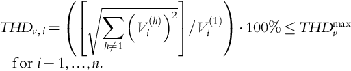
Bounds for Eq. 10-6 are specified by the IEEE-519 standard [51]. Let umax denote the maximum number of capacitor units allowed at each bus. The number of capacitors on bus i is limited by
where ufi denotes the number of fixed capacitor banks at bus i and MC is the set of possible buses for capacitor placement.
10.4.1.3 Objective Function (Cost Index)
The objective function (cost) selected for capacitor placement in the presence of harmonics is [35–37,44–46]

where
Fcap. = cost of fixed capacitors,
Fcapacity = cost corresponding to losses (e.g., used capacity of the system),
Ploss = total system losses (Eq. 10-9),
V (h) = bus voltage at harmonic h,
L = highest order of harmonics considered,
C = size of connected capacitors,
T = duration of load (hours/year),
MC = set of possible shunt capacitor buses,
Kcfp = cost per unit of fixed capacitance (Table 10.3 [37,45]),
KE = cost per MWh (e.g., KE = 50 $/MWh [40,45]), and
KA = saving per MW for reduction in losses (e.g., KA = 120,000 $/MW [40]).
Total losses can be computed using harmonic power flow output results

where Vi(h) and θi(h) are magnitude and phase of the hth harmonic voltage at bus i and yij(h) and δij(h) are magnitude and phase of hth harmonic line admittance between buses i and j, respectively.
10.4.2 Application of Maximum Sensitivities Selection (MSS) for the Capacitor Allocation Problem
This section outlines the application of maximum sensitivities selection (MSS) in conjunction with a Newton-based harmonic load flow program to generate the local solution of the capacitor placement and sizing problem in the presence of voltage and current harmonics. If the initial condition is near the global point, the MSS algorithm will generate a near global solution. Otherwise, the MSS algorithm has a high chance of getting stuck at a local point. This section introduces the application of MSS for the capacitor allocation problem as proposed by [41].
10.4.2.1 Sensitivity Functions for MSS
Sensitivities of the objective function (Eq. 10-8) to capacitance values at compensation buses can be computed using partial derivatives:

where Wh = 1/h is the weight function at harmonic h, and Ploss, k(h) are the total system losses at harmonic h for load level k and ![]() is the cost corresponding to capacitor of size Q(p + 1). Subscript p indicates the discrete step sizes of capacitor cost as listed in Table 10.3 (e.g., Q1 = 150 kVAr, Q2 = 300 kVAr, …). Note the application of linear interpolation in Eq. 10-10 due to the discrete nature of the capacitor cost (Table 10.3).
is the cost corresponding to capacitor of size Q(p + 1). Subscript p indicates the discrete step sizes of capacitor cost as listed in Table 10.3 (e.g., Q1 = 150 kVAr, Q2 = 300 kVAr, …). Note the application of linear interpolation in Eq. 10-10 due to the discrete nature of the capacitor cost (Table 10.3).
The partial derivatives of Ploss, k(h) are computed as follows:

where all right-hand side matrix entries are easily computed using the outputs of the harmonic power flow, as outlined in Chapter 7 (Section 7.4). The subscripts r and i denote real and imaginary components, respectively.
10.4.2.2 The MSS Algorithm
The shunt capacitor placement and sizing problem in the presence of linear and nonlinear loads is an optimization problem with discrete variables (e.g., discrete values of capacitors). This problem is solved using the harmonic power flow algorithm and the maximum sensitivities selection (MSS) method as follows (Fig. 10.5):

Step 1: Input system parameters (e.g., line and load specifications, system topology, and number of load levels). Select the first load level (e.g., k = 1) and set initial capacitance values at all possible compensation nodes to zero. For other load levels (k ≥ 2), use the capacitor values, computed for the preceding load levels, as the initial capacitor values of the compensation buses.
Step 2: Calculate harmonic power flow at load level k and compute the objective function (Eq. 10-8).
Step 3: Calculate sensitivities of the objective function with respect to capacitances at compensation buses (Eqs. 10-10 to 10-11).
Step 4: Select SC candidate buses with maximum sensitivities.
Step 5 (temporary change of system topology): Add one unit of capacitor to one of the candidate buses. Calculate harmonic power flow and the related objective function. Remove the newly added capacitor unit from the corresponding candidate bus.
Step 6: Repeat Step 5 for all candidate buses.
Step 7 (change of system topology): Among all candidate buses, select the one with the minimum objective function value and place one unit of capacitor at this bus. Record the corresponding system topology, F, THDv, and Vrms.
Step 8 (check convergence): If the reactive power of the total capacitance of shunt capacitors does not exceed the sum of reactive loads, the algorithm has not converged; go to Step 3.
Step 9: According to the calculated information (objective functions, THDv, and Vrms values), select the topology with the minimum objective function that satisfies the problem constraints (Eqs. 10-5 to 10-7). This is the optimal solution at load level value k. If such topology does not exist, that is, there is no solution at load level k, go to Step 11.
Step 10: Print the solution for this load level. If the final load level is not reached, select the next load level and go to Step 2.
Step 11: Stop.
10.4.2.3 Convergence of the MSS Algorithm
The burden of calculation in the MSS algorithm is much less than those of the analysis and dynamic programming (DP) methods. Assuming Nc number of capacitor units and Kc number of compensation buses, the average number of power flow calculations in DP algorithm is Kc (Kc + 1)(Nc + 1). Total number of power flow calculations of the MSS algorithm is NcKc, which is much less than that of the DP method, especially when Nc is large.
10.4.3 Application of Local Variation (LV) for the Capacitor Allocation Problem
The shunt capacitor placement and sizing problem in the presence of linear and nonlinear loads is solved using the harmonic power flow algorithm (Chapter 7, Section 7.4) and the local variations (LV) method [36]. The solution procedure as proposed by [42] is as follows (Fig. 10.6):

Step 1: Input system parameters (e.g., line and load specifications, system topology, and number of load levels). Select the first load level (e.g., k = 1).
Step 2: Select SC buses as optimal (or preferred) locations for capacitor bank placements. If such locations are not available, select all buses. Set iteration, capacitor location, and step interval numbers (i = 1, j = 1, Lj = 1). Set initial value for the optimal objective function (F* = 0).
Step 3: Start with a random combination of capacitor sizes ![]() .
.
Step 4: Set the objective function (Eq. 10-8).
Step 5: Perform harmonic power flow to compute fundamental and harmonic bus voltages.
Step 6: If power quality constraints (Eqs. 10-5 and 10-6) are satisfied go to Step 7, else:
Step 6a: If i = 1, go to Step 3 and repeat Steps 3–5 until a feasible combination is found.
Step 6b: If i ≠ 1 go to Step 8.
Step 7: Compute objective function (Eq. 10-8). If i = 1, increase i, save the objective function value (F* = F) and capacitor locations ![]() . Else, compare F with F*.
. Else, compare F with F*.
Step 7a: If F ≥ F*, go to Step 8.
Step 7b: Else, set F* ≥ F and ![]() .
.
Step 8: Change capacitor size at capacitor location j in small steps from Qo to LQo while keeping the capacitance of other capacitor locations unchanged. Repeat Steps 5–7 for each step change (Qj = LjQo, Lj = 1,…,L).
Step 9: Select a combination of capacitor sizes that corresponds to the lowest objective function (QC = QC*). This will be the starting point of Step 10.
Step 10: Repeat Steps 8 and 9 for each capacitor location (e.g., j ![]() MC).
MC).
Step 11: If solution has not converged (e.g., F* is changing in two subsequent iterations), set i = i + 1, j = 1 and repeat Steps 8–10.
Step 12: This is the optimal solution at load level k. If the final load level is reached, go to Step 14.
Step 13: Select the next load level (k = k + 1), put QC as system parameters and go to Step 2.
Step 14: Print the solution and stop.
10.4.4 A Hybrid MSS-LV Algorithm for the Capacitor Allocation Problem
Reference [42] presents a hybrid algorithm based on a combination of maximum sensitivities selection (to direct solution toward the permissible region by selecting candidate buses) and local variations (to improve accuracy). MSS is used as a fast technique to obtain the proper initial conditions for the LV method. Therefore, this algorithm takes advantage of MSS speed and LV accuracy. Unlike the LV scheme, however, its solution does not strongly depend on the initial conditions and is not limited to a local optimum. Therefore, solution accuracy is improved at the expense of more computing time.
If the initial conditions generated by the MSS method do not satisfy the power quality constraints (e.g., MSS algorithm fails to locate a solution), the proposed algorithm will apply these constraints in the second iteration of the LV algorithm.
10.4.5 Application Example 10.3: Optimal Placement and Sizing of Capacitor Banks in the Distorted 18-Bus IEEE Distribution System by MSS and MSS-LV Methods
Apply the MSS and MSS-LV algorithms of Figs. 10.5 and 10.6 to the 23 kV, 18-bus, distorted IEEE distribution system of Fig. E10.3.1. Specifications of this system are given in reference [42].

Solution to Application Example 10.3
Simulation results are shown in Table E10.3.1 and Fig. E10.3.2 for the following three operating conditions:
Table E10.3.1
Simulation Results for the 18-Bus, Distorted IEEE Distribution System (Fig. E10.3.1) at Different Distortion Levels with per Unit VA = 10 MVA, per Unit V = 23 kV, and Swing Bus Voltage = 1.05 pua
| Case 1 (high distortion) | Case 2 (medium distortion) | Case 3 (low distortion) | |||||||
| Before optimization | MSS optimization | MSS-LV optimization | Before optimization | MSS optimization | MSS-LV optimization | Before optimization | MSS optimization | MSS-LV optimization | |
| Capacitor bank | Q1 = 0.090 | Q1 = 0.090 | |||||||
| locations and | Q2 = 0.105 | Q2 = 0.030 | Q2 = 0.120 | Q2 = 0.105 | Q2 = 0.120 | Q2 = 0.120 | Q2 = 0.105 | Q2 = 0.090 | Q2 = 0.090 |
| sizes (pu) | Q3 = 0.060 | Q3 = 0.090 | Q3 = 0.060 | Q3 = 0.060 | Q3 = 0.060 | Q3 = 0.060 | Q3 = 0.060 | Q3 = 0.120 | |
| Q4 = 0.060 | Q4 = 0.180 | Q4 = 0.180 | Q4 = 0.060 | Q4 = 0.060 | Q4 = 0.060 | Q4 = 0.060 | Q4 = 0.060 | Q4 = 0.030 | |
| Q5 = 0.180 | Q5 = 0.240 | Q5 = 0.240 | Q5 = 0.180 | Q5 = 0.180 | Q5 = 0.180 | Q5 = 0.180 | Q5 = 0.180 | Q5 = 0.180 | |
| Q7 = 0.060 | Q7 = 0.120 | Q7 = 0.120 | Q7 = 0.060 | Q7 = 0.060 | Q7 = 0.060 | Q7 = 0.060 | Q7 = 0.060 | Q7 = 0.060 | |
| Q8 = 0.060 | Q8 = 0.060 | ||||||||
| Q9 = 0.030 | Q9 = 0.030 | ||||||||
| Q20 = 0.06 | Q20 = 0.09 | Q20 = 0.09 | Q20 = 0.06 | Q20 = 0.06 | Q20 = 0.06 | Q20 = 0.06 | Q20 = 0.03 | Q20 = 0.09 | |
| Q21 = 0.12 | Q21 = 0.12 | Q21 = 0.12 | Q21 = 0.12 | Q21 = 0.12 | Q21 = 0.12 | Q21 = 0.12 | |||
| Q24 = 0.15 | Q24 = 0.15 | Q24 = 0.15 | Q24 = 0.15 | Q24 = 0.15 | Q24 = 0.18 | Q24 = 0.06 | |||
| Q25 = 0.09 | Q25 = 0.03 | Q25 = 0.09 | Q25 = 0.09 | Q25 = 0.03 | Q25 = 0.09 | ||||
| Q50 = 0.12 | Q50 = 0.12 | Q50 = 0.03 | Q50 = 0.12 | Q50 = 0.09 | |||||
| Total capacitor (pu) | Qt = 1.005 | Qt = 0.900 | Qt = 0.930 | Qt = 1.005 | Qt = 1.020 | Qt = 0.990 | Qt = 1.005 | Qt = 0.630 | Qt = 0.810 |
| Minimum voltage (pu) | 1.029 | 1.016 | 1.013 | 1.044 | 1.048 | 1.043 | 1.050 | 1.020 | 1.065 |
| Maximum voltage (pu) | 1.055 | 1.056 | 1.059 | 1.062 | 1.074 | 1.071 | 1.073 | 1.050 | 1.05 |
| Maximum THDv (%) | 8.48 | 6.37 | 4.72 | 5.18 | 5.00 | 5.00 | 2.10 | 2.95 | 2.87 |
| Losses (kW) | 282.93 | 246.43 | 250.37 | 213.69 | 192.81 | 192.84 | 189.91 | 167.32 | 109.64 |
| Capacitor cost ($) | 2432.70 | 2204.7 | 2206.8 | 2432.70 | 2535.3 | 2430.3 | 2432.70 | 1754.70 | 1830.6 |
| Total cost ($/year) | 157872.98 | 137512.00 | 139710.47 | 119237.90 | 107587.47 | 107604.72 | 105969.20 | 93361.15 | 61181.74 |
| Benefits ($/year) | 20360 | 18162.51 | 11650.43 | 11633.18 | 12608 | 44787.46 | |||

a All capacitors were removed before the optimization process.

Case 1: High Harmonic Distortion
The nonlinear load in Fig. E10.3.1 is a six-pulse rectifier with active and reactive powers of 0.3 pu (3 MW) and 0.226 pu (2.26 MVAr), respectively. Results based on harmonic power flow show for this system a maximum voltage THDv of 8.48%. The MSS and MSS-LV algorithms are applied to this system for optimal placement and sizing of capacitor banks.
Results of the MSS method show a yearly benefit of $20360 (last row of Table E10.3.1) and different locations and sizes of capacitor banks before (column 2 of Table E10.3.1) and after (column 3 of Table E10.3.1) optimization. The maximum voltage THDv is only reduced to 6.37% (row 19 of Table E10.3.1 and Fig. E10.3.2). Therefore, considerable yearly benefit is achieved but power quality constraints are not satisfied.
By applying the MSS-LV algorithm, we can decrease the level of voltage THDv to 4.72% (row 19 of Table E10.3.1). As expected (due to power quality improvement), yearly benefit is slightly decreased (to $18162). If in highly harmonic distorted systems the MSS-LV algorithm does not satisfy power quality constraints, the application of passive filters and active filters (Chapter 9) before capacitor placement is recommended.
Case 2: Medium Harmonic Distortion
The size of the nonlinear load is reduced such that its active and reactive powers are 0.12 pu and 0.166 pu, respectively. After optimal placement and sizing of capacitor banks by the MSS method, voltage THDv decreases from 5.18 to 5.00% and a yearly benefit of $11650 is achieved. Applying the hybrid MSS-LV algorithm causes minor changes (e.g., eliminating one capacitor unit). Therefore, the performances of the two algorithms are similar for this case. This means that the output of MSS algorithm is near the system global solution.
Case 3: Low Harmonic Distortion
The size of the nonlinear load is further decreased such that its active and reactive powers are 0.02 pu and 0.046 pu, respectively. After optimal placement and sizing of capacitor banks by the MSS method, voltage THDv increases from 2.1 to 2.95% (which is lower than the desired limit of 3%), total capacitance of capacitor banks decreases from 1.005 to 0.63 pu, and a yearly benefit of $12608 results. By applying the MSS-LV algorithm, considerable benefit is achieved ($44787), while voltage THDv is at 2.87%.
10.4.6 Fuzzy Approach for the Optimal Placement and Sizing of Capacitor Banks in the Presence of Harmonics
All mathematical optimization methods require that the objective function be (pseudo-) convex and the constraints be (quasi-) convex. Only if convexity exists is there one optimal solution within the feasible or permissible multidimensional region. Experience teaches that the above-mentioned conditions of convexity are not necessarily met. The method of the steepest decent or ascent may lead to a conditional optimum of which several may exist due to the violation of convexity of the objective and constraint functions.
To avoid a trajectory leading to a conditional but not necessarily best conditional optimum, fuzzification of the objective and constraint functions has been introduced [44]. This process makes it possible that the solution trajectory – consisting of a band which is broad – avoids a conditional optimum, which exists due to the pseudo- or quasi-convex objective and constraint functions.
10.4.6.1 Sensitivity of Objective Function and THDv
Sensitivities of constraints and objective function are used to limit the number of calculations while a fuzzy combination of constraints and objective function is constructed to guarantee the monotonous convergence of the solution.
Sensitivity of Objective Function
Sensitivities of objective function (Eq. 10-8) to capacitance values at compensation buses can be computed using Eqs. 10-10 and 10-11.
Sensitivity of THDv
Sensitivities of THDv (Eq. 10-6) to capacitance values at compensation buses is computed using the partial derivatives

where Wh = 1/h is the proposed weighting function for harmonic order h. The partial derivatives of THDv,j are computed as follows:

where all right-hand-side matrix entries are easily computed using results from the application of a harmonic power flow program.
10.4.6.2 Fuzzy Implementation
Fuzzy set theory (FST) is relied on to determine the candidate buses and to select the most suitable bus for capacitor placement.
Fuzzification of Sensitivities
For the sensitivities of objective function (Eqs. 10-10 and 10-11) and constraints (Eqs. 10-12 and 10-13) with respect to the reactive power injection at each bus, the exponential fuzzifier functions ![]() are employed. Figure 10.7a shows the fuzzifier for the sensitivity of THDv,j. STHDmax is a large number, that is, buses with higher sensitivities have higher values of membership.
are employed. Figure 10.7a shows the fuzzifier for the sensitivity of THDv,j. STHDmax is a large number, that is, buses with higher sensitivities have higher values of membership.

Fuzzification of Objective Function and Constraints
For the objective function (Eq. 10-8) a membership function (μF) is defined as depicted in Fig. 10.7b. Fo is the initial value of objective function and F1 is the value of objective function after compensating the total reactive (inductive) loads at every bus of the distribution system. High objective values are given a low membership function value, whereas low objective values are assigned a high membership function value.
For voltage constraints, it is suitable to use a membership function (μv,j) with trapezoidal form, as shown in Fig. 10.7c. Vmin and Vmax correspond to Eq. 10-5 such that buses with voltages values between the two limit values Vmin and Vmax have full membership. ![]() and
and ![]() correspond to initial values of the bus effective voltage. Therefore, a bus with high rms voltage deviation (Eq. 10-5) is given a low value and a bus with low rms voltage deviation is given a high value.
correspond to initial values of the bus effective voltage. Therefore, a bus with high rms voltage deviation (Eq. 10-5) is given a low value and a bus with low rms voltage deviation is given a high value.
For THDv,j a membership function (μTHDv,j) is defined as illustrated in Fig. 10.7d. THDvmax and THDv0 are the limit and the initial value of THDv,j corresponding to Eq. 10-6, respectively. Buses are given a high value (e.g., μTHDv,j = 1) unless their THDv are higher than the IEEE-519 limits.
Fuzzy Combination of Membership Functions
The algebraic product of the membership functions is used such as the t-norm for THDv,j:

The same formulations apply to t-norms of the bus voltages, sensitivity of THDv,j and sensitivity of voltage constraints, the combination of objective function and constraints, as well as their sensitivities to reactive power injection:
Alpha-Cut Process
In order to direct the algorithm toward the permissible region bordered by constraints, the α-cut process is used at each iteration. To do this, the values of α for F, THDv, and V are set to their corresponding membership values in the previous iteration (e.g., ![]() where ℓ is the iteration number).
where ℓ is the iteration number).
Analysis
The initial starting point of Eq. 10-8 (e.g., the initial compensation buses) does not usually reside inside the permissible solution region. Therefore, some type of criteria (based on simultaneous improvements of F, THDv, and V in consecutive iterations) is required to direct the solution toward the permissible region and to select the most appropriate buses for capacitor placement. This section uses the fuzzy set theory to measure individual improvements, generate a single criterion to direct the solution, and guarantee the monotonous convergence of the solution at each iteration. Other approaches with similar characteristics (e.g., analytical hierarchy process) could also be used.
Note that the locations of candidate buses as indicated by the sensitivities of F, THDv, and V are usually different. A single criterion – a fuzzy combination – is employed to determine the optimal locations of candidate buses. The exponential sensitivity functions of Fig. 10.7a are solely used for ranking of candidate buses. Other methods could be employed for this ranking (e.g., weighted average, statistical methods). The selected method will not have any impact on the capacitor placement algorithm. However, the selected trapezoidal membership functions of Fig. 10.7b–d for F, V, and THDv have major impacts on the solution process (e.g., improving or deteriorating convergence).
The inclusion of sensitivity functions and fuzzification of objective and power quality constraints will automatically eliminate all solutions generating extreme values of voltages and/or currents and prevents fundamental and harmonic parallel resonances.
10.4.6.3 Solution Methodology
The shunt capacitor placement and sizing problem in the presence of linear and nonlinear loads is an optimization problem with discrete variables (e.g., discrete values of capacitors). This problem is solved using the harmonic power flow algorithm and the fuzzy set theory (Fig. 10.8) as follows:

Step 1: Input system parameters (e.g., line and load specifications and system topology). Initial capacitor values of all possible compensation buses are set to zero.
Step 2: Calculate harmonic power flow.
Step 3: Evaluate the objective function (Eq. 10-8), sensitivities of objective function, constraints, and their fuzzy combination (Eq. 10-15a) in order to determine the list of candidate buses.
Step 4: Sort candidate buses (CB) and from among them select several buses with maximum sensitivities and total number of installed capacitor banks less than umax.
Step 5: Apply α-cut process and compute the membership functions for the objective function and constraints with respect to the present topology.
Step 6: Add one unit of capacitor to one of the candidate buses. Calculate harmonic power flow and record the values of related membership functions. Remove the newly added capacitor unit from the corresponding candidate bus.
Step 7: Repeat Step 6 for all other candidate buses.
Step 8: If all total membership functions are zero, go to Step 11.
Step 9: Among all candidate buses, select the one with maximum value of total membership function and place one unit of capacitor at this bus.
Step 10: If the reactive power of the total capacitance of shunt capacitors does not exceed the sum of reactive loads and the total number of installed capacitor banks are less than Umax, go to Step 2.
Step 11: Print the solution and stop.
10.4.7 Application Example 10.4: Optimal Placement and Sizing of Capacitor Banks in the Distorted 18-Bus IEEE Distribution System by Fuzzy Expert System
Apply the MSS and fuzzy algorithms of Figs. 10.5 and 10.8 for capacitor placement and sizing to the 23 kV, 18-bus, distorted IEEE distribution system of Fig. E10.3.1.
Solution to Application Example 10.4
Simulation results are compared in Table E10.4.1 for the following operating conditions.
Table E10.4.1
Simulation Results for the 18-Bus, Distorted IEEE Distribution System (Fig. E10.3.1) at Different Distortion Levels with Per Unit S = 10 MVA, per Unit V = 23 kV, and Swing Bus Voltage = 1.05 pua
| Case 1 (high distortion) | Case 2 (low distortion) | |||||
| Before optimization | After MSS optimization | After fuzzy optimization | Before optimization | After MSS optimization | After fuzzy optimization | |
| Capacitor bank | Q2 = 0.105 | Q2 = 0.030 | Q2 = 0.015 | Q2 = 0.105 | Q2 = 0.090 | |
| locations and | Q3 = 0.060 | Q3 = 0.090 | Q3 = 0.030 | Q3 = 0.060 | Q3 = 0.255 | |
| sizes (pu) | Q4 = 0.060 | Q4 = 0.180 | Q4 = 0.060 | Q4 = 0.060 | Q4 = 0.060 | Q4 = 0.030 |
| Q5 = 0.180 | Q5 = 0.240 | Q5 = 0.240 | Q5 = 0.180 | Q5 = 0.180 | Q5 = 0.060 | |
| Q7 = 0.060 | Q7 = 0.120 | Q7 = 0.210 | Q7 = 0.060 | Q7 = 0.060 | Q7 = 0.030 | |
| Q20 = 0.060 | Q20 = 0.090 | Q20 = 0.090 | Q20 = 0.060 | Q20 = 0.030 | Q20 = 0.165 | |
| Q21 = 0.120 | Q21 = 0.120 | Q21 = 0.120 | Q21 = 0.120 | Q21 = 0.015 | ||
| Q24 = 0.150 | Q24 = 0.150 | Q24 = 0.180 | Q24 = 0.075 | |||
| Q25 = 0.090 | Q25 = 0.030 | Q25 = 0.090 | Q25 = 0.030 | Q25 = 0.045 | ||
| Q50 = 0.120 | Q50 = 0.120 | |||||
| Total capacitor (pu) | Qt = 1.005 | Qt = 0.900 | Qt = 0.765 | Qt = 1.005 | Qt = 0.630 | Qt = 0.675 |
| Minimum voltage (pu) | 1.029 | 1.016 | 0.998 | 1.050 | 1.020 | 1.021 |
| Maximum voltage (pu) | 1.055 | 1.056 | 1.050 | 1.073 | 1.050 | 1.054 |
| Max. THDv (%) | 8.48 | 6.37 | 4.89 | 2.10 | 2.95 | 2.63 |
| Losses (kW) | 282.93 | 246.43 | 257.46 | 189.91 | 167.32 | 160.48 |
| Capacitor cost ($/year) | 1978.2 | 1692 | 1458.30 | 1978.20 | 1311.90 | 1538.25 |
| Total cost ($/year) | 159853.14 | 139199.94 | 145120.98 | 107947.98 | 94676.46 | 91086.09 |
| Benefits ($/year) | 20653 | 14732 | 13271 | 16861 | ||
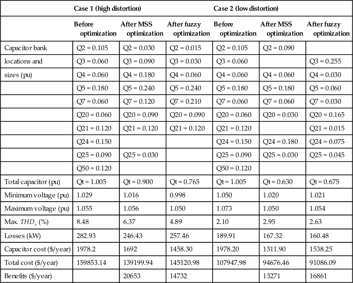
a All capacitors were removed before the optimization process.
Case 1: High Harmonic Distortion
The nonlinear load in Fig. E10.3.1 is a six-pulse rectifier with active and reactive powers of 0.3 pu (3 MW) and 0.226 pu (2.26 MVAr), respectively. Results of harmonic power flow indicate a maximum voltage THDv of 8.48% for this system (column 2 of Table E10.4.1).
Application of the MSS method to Fig. E10.3.1 shows that optimal capacitor placement results in considerable yearly benefit (e.g., $20653 per year) but it does not limit THDv to the desired level of 5% (column 3 of Table E10.4.1). This is expected from the MSS method dealing with rich harmonic configurations, where capacitor placement is not the primary solution for harmonic mitigation.
The fuzzy algorithm of Fig. E10.3.1 is also applied to this system for optimal placement and sizing of capacitor banks. Results show a yearly benefit of $14732 per year (last row of Table E10.4.1) and different locations and sizes of capacitor banks before (column 2 of Table E10.4.1) and after (column 4 of Table E10.4.1) the fuzzy optimization. In addition, maximum voltage THDv is reduced to 4.89% (row 16 of Table E10.4.1) and total capacitance is decreased by 24%.
Case 2: Low Harmonic Distortion
The size of the nonlinear load is decreased such that its active and reactive powers are 0.02 pu and 0.046 pu, respectively. After optimal placement and sizing of capacitor banks with MSS method, THDv increases from 2.1 to 2.95% (which is lower than the desired limit of 5%), total capacitance of capacitor banks is decreased from 1.005 pu to 0.630 pu and a yearly benefit of $13271 is achieved (column 6 of Table E10.4.1).
Application of the fuzzy algorithm results in THDv increase from 2.1 to 2.63% (which is in the permitted region) and also total capacitance decreases from 1.005 to 0.675 pu (column 7 of Table E10.4.1). In addition, annual savings are increased to $16861 (e.g., 27% greater savings than that of the MSS method). These results demonstrate the fine capability of the fuzzy method for capacitor placement in the presence of harmonics.
10.4.8 Optimal Placement, Replacement, and Sizing of Capacitor Banks in Distorted Distribution Networks by Genetic Algorithms
Most traditional optimization approaches use deterministic rules to move from one point in the decision hyperspace to another point and will likely get stuck at a local optimum. GAs start with a diverse set of potential solutions that allows for exploration of many optima in parallel, lowering the probability of getting stuck at a local optimum. Even though GAs are probabilistic, they are not strictly random searches. The stochastic operators used on the population direct the search toward regions of the hyperspace that are likely to have higher fitness values.
This section presents a genetic method to formulate the capacitor placement and sizing problem in the presence of voltage and current harmonics, taking into account fixed capacitors with a limited number of capacitor banks at each bus and the entire feeder [45]. Operational and power quality constraints include bounds for rms voltage, THDv, and the number and size of installed capacitors.
10.4.8.1 Genetic Algorithm
Genetic algorithms use the principles of natural evolution and population genetics to search and arrive at a near global solution. The required design variables are encoded into a binary string as a set of genes corresponding to chromosomes in biological systems. Unlike traditional optimization techniques that require one starting point, GAs use a set of points as initial conditions. Each point is called a chromosome. A group of chromosomes is called a population. The number of chromosomes in a population is usually selected to be from 30 to 300. Each chromosome is a string of binary codes (genes) and may contain substrings. The merit of a string is judged by the fitness function, which is derived from the objective function and is used in successive genetic operations. During each iterative procedure (referred to as a generation), a new set of strings with improved performance is generated relying on three GA operators (i.e., reproduction, crossover, and mutation).
Structure of Chromosomes
Different types of chromosomes for GAs have been proposed and implemented. This section employs the chromosome structure of Fig. 10.9 consisting of MC substrings of binary numbers, where MC denotes the number of possible compensation (candidate) buses for capacitor placement in the entire feeder. The binary numbers indicate the size of the installed capacitor at the bus under consideration.

Fitness Functions
The inverse algebraic product of penalty functions (Fig. 10.10) is used as the fitness function combining objective and constraint functions:

where penalty functions FF, FTHDv,j, Fv,i, and FU are shown in Fig. 10.10.

Genetic Operators
Three genetic operators including reproduction (based on the roulette-wheel mechanism), crossover (with crossover probability of 0.6 to 1.0), and mutation (with mutation probability of 0.01 to 0.1) are established.
Convergence Criterion
The iterations (regenerations) of the genetic algorithm are continued until all generated chromosomes become equal or the maximum number of iterations (Nmax = 40) is reached. Due to the randomness of the GA method, the solution tends to differ for each run, even with the same initial population. Therefore, multiple runs are performed and the most acceptable solution (with most benefits within the permissible region of constraints) is selected.
10.4.8.2 Solution Methodology
The shunt capacitor placement and sizing problem in the presence of linear and nonlinear loads is solved based on the genetic algorithm of Fig. 10.11 as follows:
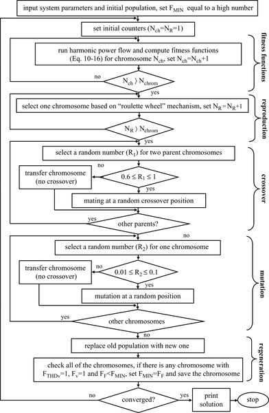
Step 1: Input system parameters (e.g., system topology, line and load specifications). Input the initial population with Nch chromosomes.
Step 2: Set initial counter and parameter values (e.g., Nch = Nit = NR = 1 and FMIN = a high number).
Step 3 (Fitness Process):
Step 3a: Run harmonic power flow for Nch chromosomes and save results.
Step 3b: Compute proposed penalty functions (Fig. 10.10) employing data generated by harmonic power flow program. Compute fitness functions (Eq. 10-16) for chromosome Nch. Set Nch = Nch + 1.
Step 3c: If Nch ≤ Nchrom go to Step 3a.
Step 4 (Reproduction Process):
Step 4a: Define total fitness as the sum of all fitness values for all chromosomes.
Step 4b: Select a percentage of “roulette wheel” for each chromosome that is equal to the ratio of its fitness value to the total fitness value.
Step 4c: Improve generation by rolling the roulette wheel Nch times. Select a new combination of chromosomes.
Step 5 (Crossover Process):
Step 5a: Select a random number (R1) for mating two parent chromosomes.
Step 5b: If R1 is between 0.6 and 1.0 then combine the two parents, generate two offspring, and go to Step 5d.
Step 5c: Else, transfer the chromosome with no crossover.
Step 5d: Repeat steps 5a to 5c for all chromosomes.
Step 6 (Mutation Process):
Step 6a: Select a random number (R2) for mutation of one chromosome.
Step 6b: If R2 is between 0.01 and 0.1 then apply the mutation process at a random position and go to Step 6d.
Step 6c: Else, transfer the chromosome with no mutation.
Step 6d: Repeat steps 6a to 6c for all chromosomes.
Step 7 (Updating Populations): Replace the old population with the improved population generated by Steps 2 to 6. Check all chromosomes; if there is any chromosome with FTHDv = 1, Fv = 1, and FF < FMIN, set FMIN = FF and save it. Set Nit = Nit + 1.
Step 8 (Convergence): If all chromosomes are the same or the maximum number of iterations is reached (Nit = Nmax), then print the solution and stop, else go to Step 2.
10.4.9 Application Example 10.5: Optimal Placement and Sizing of Capacitor Banks in the 6-Bus IEEE Distorted System
Apply the MSS, MSS-LV, fuzzy, and genetic algorithms of Figs. 10.5, 10.6, 10.8 and 10.11 for capacitor placement and sizing to the 69 kV, 6-bus, distorted IEEE distribution system of Fig. E10.5.1. Specifications of this system are given in reference [42].

Solution to Application Example 10.5
Simulation results are compared in Table E10.5.1. The nonlinear load in Fig. E10.5.1 is a six-pulse rectifier with active and reactive powers of 0.2 pu (2 MW) and 0.25 pu (2.5 MVAr), respectively. Results of a harmonic power flow program indicate a maximum voltage THDv of 5.270% (column 2 of Table E10.5.1).
Table E10.5.1
Simulation Results for the 6-Bus, Distorted IEEE System of Fig. E10.5.1 with Base Apparent Power S = VA = 10 MVA, Base Voltage V = 69 kV, and Swing Bus Voltage = 1.00 pua
| Before optimization | After MSS optimization | After MSS-LV optimization | After fuzzy optimization | After GA optimization | |
| Capacitor bank locations and sizes (pu) | Q1 = 0.000 Q2 = 0.000 Q3 = 0.000 Q4 = 0.000 Q5 = 0.000 Q6 = 0.000 | Q1 = 0.000 Q2 = 0.000 Q3 = 0.000 Q4 = 0.000 Q5 = 0.150 Q6 = 0.000 | Q1 = 0.405 Q2 = 0.000 Q3 = 0.315 Q4 = 0.000 Q5 = 0.150 Q6 = 0.000 | Q1 = 0.000 Q2 = 0.000 Q2 = 0.000 Q4 = 0.000 Q5 = 0.135 Q6 = 0.000 | Q1 = 0.120 Q2 = 0.000 Q3 = 0.45 Q4 = 0.00 Q5 = 0.405 Q6 = 0.000 |
| Total capacitor (pu) | Qt = 0.000 | Qt = 0.150 | Qt = 0.870 | Qt = 0.135 | Qt = 0.405 |
| Minimum voltage (pu) | 0.935 | 0.965 | 1.000 | 0.962 | 0.996 |
| Maximum voltage (pu) | 1.005 | 1.013 | 1.070 | 1.012 | 1.044 |
| Maximum THDv (%) | 5.270 | 5.007 | 4.970 | 4.990 | 4.943 |
| Losses (kW) | 360 | 295 | 285.2 | 299 | 276.7 |
| Capacitor cost ($/year) | 0.00 | 301.50 | 1640.7 | 279.45 | 725.85 |
| Total cost ($/year) | 200880.0 | 164911.5 | 160782.0 | 167121.45 | 155101.85 |
| Computing time (sec)b | - | 6 | 115 | 10 | 639 |
| Benefits ($/year) | 35968.5 | 40098.0 | 33758.55 | 45778.15 |

a All capacitors were removed before the optimization process.
b Using a Pentium III (550 MHz) personal computer.
After optimal placement and sizing of capacitor banks with the MSS algorithm, the voltage THDv decreases to 5.007% by allocating 0.15 pu capacitor banks and a yearly benefit of $35968 is achieved (column 3 of Table E10.5.1). Applying the MSS-LV algorithm to the system yields a yearly benefit of $40098 and a voltage THDv of 4.970 (column 4 of Table E10.5.1). Optimization of the system based on the fuzzy set algorithm generates voltage THDv of 4.990% and a yearly benefit of $33758 (column 5 of Table E10.5.1). Application of the genetic algorithm (with Nch = 100) results in about the same voltage THDv (e.g., 4.943%), and the annual savings are increased to $45778 (column 6 of Table E10.5.1).
10.4.10 Application Example 10.6: Optimal Placement and Sizing of Capacitor Banks in the 18-Bus IEEE Distorted System
Apply the MSS, MSS-LV, fuzzy, and genetic algorithms of Figs. 10.5, 10.6, 10.8 and 10.11 for capacitor placement and sizing to the 23 kV, 18-bus, distorted IEEE distribution system of Fig. E10.3.1. Specifications of this system are given in reference [42]. The nonlinear load in Fig. E10.3.1 is a six-pulse rectifier with active and reactive powers of 0.3 pu (3 MW) and 0.226 pu (2.26 MVAr), respectively.
Solution to Application Example 10.6
Results of a harmonic power flow program show a maximum voltage THDv of 8.486% for this system (column 2 of Table E10.6.1). Application of MSS method to Fig. E10.3.1 shows that optimal capacitor placement results in considerable yearly benefit (e.g., $20653 per year), but it does not limit voltage THDv to the desired level of 5% (column 3 of Table E10.6.1). Applying the MSS-LV algorithm yields a yearly benefit of $17939 and voltage THDv is reduced to 4.72% (column 4 of Table E10.6.1). Application of the fuzzy algorithm results in an acceptable voltage THDv level and benefits (4.899% and $14732, column 5 of Table E10.6.1).
Table E10.6.1
Simulation Results of MSS, MSS-LV, Fuzzy, and Genetic Algorithms for the 18-Bus, Distorted IEEE Distribution System (Fig. E10.3.1) with per Unit VA = 10 MVA, per Unit V = 23 kV, and Swing Bus Voltage = 1.05 pua
| Before optimization | After MSS optimization | After MSS-LV optimization | After fuzzy optimization | After GA optimization | |
| Capacitor bank locations and sizes (pu) | Q2 = 0.105 Q3 = 0.060 Q4 = 0.060 Q5 = 0.180 Q7 = 0.060 Q20 = 0.060 Q21 = 0.120 Q24 = 0.150 Q25 = 0.090 Q50 = 0.120 | Q2 = 0.030 Q3 = 0.090 Q4 = 0.180 Q5 = 0.240 Q7 = 0.120 Q20 = 0.090 Q21 = 0.120 Q24 = 0.000 Q25 = 0.030 Q50 = 0.000 | Q2 = 0.120 Q3 = 0.060 Q4 = 0.180 Q5 = 0.240 Q7 = 0.120 Q20 = 0.090 Q21 = 0.120 Q24 = 0.000 Q25 = 0.000 Q50 = 0.000 | Q2 = 0.015 Q3 = 0.030 Q4 = 0.060 Q5 = 0.240 Q7 = 0.210 Q20 = 0.090 Q21 = 0.120 Q24 = 0.000 Q25 = 0.000 Q50 = 0.000 | Q2 = 0.030 Q3 = 0.000 Q4 = 0.165 Q5 = 0.330 Q7 = 0.105 Q20 = 0.060 Q21 = 0.090 Q24 = 0.015 Q25 = 0.015 Q50 = 0.030 |
| Total capacitor (pu) | Qt = 1.005 | Qt = 0.900 | Qt = 0.930 | Qt = 0.765 | Qt = 0.840 |
| Minimum voltage (pu) | 1.029 | 1.016 | 1.013 | 0.998 | 1.003 |
| Maximum voltage (pu) | 1.055 | 1.056 | 1.059 | 1.050 | 1.050 |
| Maximum THDv (%) | 8.486 | 6.370 | 4.720 | 4.899 | 4.883 |
| Losses (kW) | 282.93 | 246.43 | 250.37 | 257.46 | 249.31 |
| Capacitor cost ($/year) | 1978.20 | 1692.00 | 2206.80 | 1458.30 | 1788.75 |
| Total cost ($/year) | 159853.14 | 139199.94 | 141913.26 | 145120.98 | 140903.73 |
| Computing time (sec)b | – | 96 | 141 | 48 | 2780 |
| Benefits ($/year) | 20653.6 | 17939.88 | 14732.16 | 18949.41 |

a All capacitors were removed before the optimization process.
b Using a Pentium III (550 MHz) personal computer.
The genetic algorithm (GA) of Fig. 10.11 is also applied to this system for optimal placement and sizing of capacitor banks (Nch = 250). Results reveal a yearly benefit of $18949 (last row of Table E10.6.1); maximum voltage THDv is limited to 4.880% (column 6 of Table E10.6.1), and the total allocated capacitance is decreased by 16%.
Greater power quality control mitigation is achieved with the GA at the expense of lower benefits compared with the MSS solution. The GA yields greater yearly benefits while the power quality conditions are the same than those of the MSS-LV solution. Compared with the fuzzy solution, the same power quality conditions result (rows 12–15 of Table E10.6.1), but greater benefits (e.g., 28% greater savings) are achieved with GA.
The results of Tables E10.5.1 and E10.6.1 indicate that the genetic algorithm captures more advantageous solutions than the MSS, MSS-LV, and fuzzy algorithms. This is expected because the genetic algorithm has the capability of computing the near global solution.
Computing Time
Unfortunately, the application of GAs often looks like a never-ending process. In fact, only a compromise between population size, mutation rate, and so on can lead to an adequate algorithm that finds good solutions in a relatively short time. However, capacitor bank placement is usually considered a planning problem and its computing time is not of great concern. The computational burden associated with the genetic algorithm is included and compared with those of the MSS, MSS-LV, and fuzzy methods as shown in row 15 of Table E10.5.1 and row 19 of Table E10.6.1. As expected, the computing times of the genetic algorithm are much longer.