
chapter four Processes
So it is, said the Wise Eagle, that the river, like the flow of things, is always the same despite being different every day.
Darloz
4.1 Introduction to Chapter 4
Processes and methods have long been an integral part of project management, the critical path analysis and critical incidents path analysis being two examples among others. The Project Management Body of Knowledge (PMBOK) 5 defines processes (p. 85) as “a set of interrelated actions and activities performed to create a prespecified product, service, or result. Each process is characterized by its inputs, the tools and techniques that can be applied, and the resulting outputs.”
On pages 11 and 12, it exemplifies processes in the following terms:
A primary function of a PMO (Project Management Office) is to support project managers in a variety of ways which may include, but are not limited to: managing shared resources across all projects administered by the PMO.
PMBOK 5 also refers to best practices, methodology, policies, procedures standards, and templates.
Processes apply to concrete items such as building materials just as much as to abstract elements or information. In the latter case, data constitute the input. This input goes through a transformation stage, such as collect → sort → analyze → synthesize → use for decision-making → use for action → use to evaluate → archive. The output is the actual document that is being shelved or archived. All processes contain these three fundamental elements: inputs, transformation, and outputs.
This chapter delves into the minutiae of processes, a subject we have briefly touched on in the frames of analysis discussed in the context of prefeasibility studies.
4.2 Transformation
As we have seen in the previous chapters, processes1 is one of the four Ps (Plans, Processes, People, and Power) of a feasibility study and of project management. Nature has its own processes: two prime examples are parasitism and symbiosis, which are strategies for life survival. Processes, in their most simple expression, consist of leading inputs into a change phase out of which they come as outputs that serve a certain utility, which is embedded in the notion of opportunity. Some sources of reference classify outputs as benefits, ordinary outputs, and results.2 From our perspective, the results are either products, processes, services, or scientific research, and benefits are most likely tied to financial value or utility.
Transformation is a utilitarian act or else a series of acts. We touched on the idea that utility may be linked to “efficiency” and “efficacy”, two terms we will define further along in this chapter. The notion of utility is fundamental; it is vastly used in economics, and we will see in Chapters 5 and 6 that we can resort to it when addressing interpersonal relationships. Put simply, if there were no utility in a project, there would be no successful project. In my initial model, I stated that a key characteristic of projects is that they answer particular needs or, viewed differently, that they respond to opportunities. However, in the end, this response must have a utility. Utility is bound in particular by a calendar of tasks and activities. This is another fundamental aspect of projects. In classical economic science, time is generally not a factor to be reckoned with when discussing utility curves; in project management, time is of the essence. I will come back to this notion of utility and see its relationship to the k constant in the section on efficiency.
We have also seen that some modeling comes in handy when wanting to simplify complex processes and guarantee that stakeholders relate to the project in the same way, thus avoiding confusion once the team members (the Forces of Production, FP) become actively involved. Before we venture too far into the specifics of Processes, we must learn how to create a utility model of the transformation phase. This is what we do next.
4.3 Modeling processes
Various authors have commented on the usefulness of modeling. It has been said, for example, that
Regardless of the kind of reliability and validity checks, models are simplifications of reality. They can be made more or less complicated and may capture all or only a portion of the variance in a given set of data. It is up to the investigator and his or her peers to decide how much a particular model is supposed to describe.3
Other scholars specify that modeling be done by grouping concepts while ensuring a sense of coherence, explaining by the same token that modeling is a simplification of reality.4 Some authors rightfully comment that modeling is meant to make intelligible a complex reality, not to make complexity a simple reality. Overall, the key concern is to achieve simplification. I propose a method that allows feasibility experts to simplify complex processes.
There are, of course, several ways to model processes. Nowadays, the program evaluation and review technique (PERT) is losing ground in favor of the Critical Path Method5 (CPM). On the other hand, dynamic systems simulation offers opportunities for rich optimizations.
As can be guessed by the reader, I have stuck to a certain number of rules when illustrating the project makeup in the chapters covered so far. Indeed, I use the modeling system that I find most useful because it allows the analyst to detect holes (or POVs) within the model under investigation.6 When it comes to processes, this method calls for parallelograms and arrows. I detail it in the next subsections. The explanations may seem a bit dry because they rest on a set of rules and procedures, but I find it to be a necessary analytical method in order to pinpoint POVs.
4.3.1 Straight direct and diagonal flows
There are two important flows in the transformation phase that need to be taken into account and that are most often ignored. All processes can be divided into two directional flows: straight direct or diagonal. Dominant and Contingency strategies are examples of straight direct processes because things are prepared and evolve according to plan; a Short strategy is an example of a diagonal process because the manager is caught off guard and must resort to innovative ways to get out of trouble.
Production processes that use machinery are generally of the so-called straight direct kind: there is one point of entry, one direction in the production, and one output. There could be various points of entry; for example, in some corrugated carton manufacturing, two corrugated cardboard sheets of corrugated carton of different sizes enter from different entry points to be channeled along some conveyors bordered by rails. Eventually, these two sheets are glued together to produce one single box that can be folded in various ways, much like a piece of origami. This remains a straight direct flow. The bottom line is that the inputs are not diverted; they adopt a linear logic that leads them toward a predictable output. To revert to the example of the chess game, straight direct flows can be represented by the rooks. In a good strategic game, rooks are generally deployed once other pieces on the board have been assigned a fair or an advantageous strategic position. From a managerial point of view, this means that the transformation phase, which should be, in theory, completely direct linear, should be deployed once all the other strategic steps have been put in place; that is, once the four Ps have been properly prepared for it. POVs become obvious when the direct linear process starts going awry; if it does, it may be caused by uncontrollable factors that have awakened preexisting POVs lying dormant within the four Ps.

Diagonal processes are typical of human thinking and interaction. Group meetings provide a prime example: a meeting rarely evolves as anticipated. One participant starts to wander, another one diverts to an unrelated topic, and so forth. Diagonal processes seem counterproductive, but in fact, they are an essential part of any project. Each project is unique and contains some level of innovation. Innovation is, by definition, a diagonal process. These occur when one walks off track, that is, when one explores avenues that are not commanded by the routine aspects of life, that have not been planned, that provide new information, and that may, in the end, change the ultimate outcome of the transformation process. Hence, while straight direct processes ensure that the ultimate outcome is what was 100% forecasted, diagonal processes show deviations from the forecasted output. Diagonal processes resemble the way that a bishop moves on a chessboard. Strategically, they are deployed on the board before the rooks and they often play a pinning role: they prevent one piece from moving (e.g., they attack a knight that is in line with the queen so that moving the knight leads to the loss of the queen).
As strange as it seems, straight direct processes present some disadvantages, especially in the area of work culture (psychodynamics; i.e., the way people interact). The groupthink phenomenon is a case in point: members of a group convince themselves that they are correct even when they are wrong. Why? Because they wish to remain as consistent with themselves as possible (a logic exemplified by the k constant). On the other hand, a machine that goes off tangent and throws inputs into different diagonal directions will not produce the anticipated output.
Overall, straight direct and diagonal flows both play a vital role in the transformation process. Typically, most diagonal processes should take place before and at the beginning of the transformation phase, and most straight direct flows should occur during and at the end of the transformation phase. A project is in large part a melting pot of straight direct and diagonal processes. POVs can be detected when this combination starts to be both ineffective and inefficient. A feasibility study should recognize which processes are straight direct and which ones are diagonal, and in fact, it should corroborate the fact that a project plan accounts for both during the entire transformation phase. In other words, some brainstorming sessions during the construction phase are always good, if it were only to discover what goes right (not what goes wrong) in the project.*
An example of such a dynamic between straight direct and diagonal flows is the Apollo 13 mission. All was set in a linear fashion—a straight direct process. However, a problem with an oxygen tank occurred during the flight that forced engineers to think outside the box in order to save the crew and bring it back to earth. It is through a diagonal process that this was achieved—by way of imagining ways of dealing with carbon dioxide and a shortage of oxygen. Technically, the idea of using the moon’s gravity to produce a string shot effect is also a diagonal process, given the circumstances. Often, diagonal processes are integrated to become straight direct processes in future ventures. According to Darwin’s theory of evolution, it is changes in the normal flow of heredity (diagonal processes) that lead to random improvements which, if they warrant better prospects of survival, will eventually be adopted (become linear processes). Hence, evolution dictates straight direct and diagonal flows.
POVs are brought under control when straight direct and diagonal processes work in tandem to achieve a result that is close enough to the intended output. They become a source of problems when the two processes interfere with each other. Because diagonal flows are mostly intangibles as they often pertain to psychological phenomena, one cannot actually exactly measure them, but we will see in Chapters 5 and 6 on People how we can go around this hurdle.
4.3.2 Parallelograms
Parallelograms apply to any element of a process and arrows are used to illustrate the bonds that exist between each process element, or put differently, between each parallelogram.
Parallelograms have various codes. All models develop from a starting point, the beginning parallelogram is always drawn with a thick outline. The intermediate parallelograms do no use thick outlines and the end parallelogram is filled in black. The best example is that of the basic definition of a project as shown in Figure 4.1.

Recall that processes are so-called straight direct, that is, they are linear and without any interruptions; any process that does not respect this assumption should be redesigned in a way that meets this condition. This may require looking at the project in a different way. This is a crucial effort because it eases the detection of POVs. A POV that is hidden in a variety of entry points, end points, or nondirect flows will likely remain undetected until after it causes damage to the project. However, with a straight direct process, the human brain can easily track the problems and their consequences using a back and forth analysis.
The bond that links the parallelograms is, in these cases as in any such project model, coordinated by time (T). It is called a “longitudinal” bond and has no polarity (it is neither positive nor negative). However, there is a system where there is a feedback loop to the entry point (or other points along the transformation stages). In this case, the time factor is expressed by a small t, or more exactly (t). In some software modeling systems (e.g., in some electrical software), a small r is sometimes used. I adopt the (t) nomenclature in my modeling system.
A typical feedback loop is found in the closed dynamic system that is a hospital. The patient first sees the doctor; then, based on the assessment of his ailment, a bed is reserved for a predetermined period of time, and surgery is scheduled. Costs accompany such a flow of events. The patient will have no choice but to go back (feedback loop) to his/her doctor in order to have his/her recovery assessed and receive permission to leave the hospital.
There are two other kinds of bonds that also contain a time factor: influence (I) and causal (C). I and C bonds have polarity: there may be a positive or negative influence of one parallelogram (project element) on another one (I+ or I−), and one parallelogram may cause another parallelogram to exist with positive or negative results (C+ or C−). Hence, we arrive at Table 4.1.7
| Name of bond involving time | Code |
|---|---|
| Longitudinal | (T) |
| Longitudinal (loop back) | (t) |
| Influence | (I+) or (I−) or (I±) |
| Causal | (C+) or (C−) |
All three types of bonds (T, I, and C) are named consequent arrows; as indicated, they mandatorily imply a temporal factor.8 These bonds are consequent in the sense that they lead one parallelogram (project element) to another, either because this will obligatorily happen over time (T), or because one project element influences another over time (I), or else one project element causes the emergence of the other one over time, 100% of the time, given a set of conditions (C). As an example of the latter dynamic, let us take a simple kettle. Placed over fire, it will bring the water it contains to boiling point 100% of the time, given the right heat and atmospheric pressure conditions. There is just no way around it, every single time the conditions are met, the process will take place.
So far, we have what is illustrated in Figure 4.2.

As a rule of thumb, “time” is assumed to travel left to right; project elements must follow their sequence from left to right.9 Note that each arrow in any model must be identified, as in Figure 4.2; this is done by way of inserting either (T), (I), or (C) with their respective polarities wherever they apply. This way, anyone can capture the dynamic that links the project elements together.
4.3.3 Corrugated cat litter box example
As an example of a straight direct flow, I will discuss a cat litter corrugated box. Let me first give the background for this innovative product.
As of 2014, U.S. citizens own more than 70 million domestic cats; Canadians own about one-tenth this number. The pet product market is continuously expanding and has the advantage of being countercyclical: when the economy turns sour, people seek companionship and buy more pet products. In England, pet owners spend more on pet food than on their own breakfast.
Cats behave quite differently than dogs. Stray cats can survive; most stray dogs cannot. Cats take great care in maintaining their fur and in using clean waste disposal facilities—cat litter boxes. Cats will not hesitate to boycott dirty cat litter trays. Hence, a cat owner must routinely clean the cat litter tray with a small scoop or else throw the entire litter content away (typically composed of urine- and feces-filled sodium bentonite). This is an unpleasant chore because the litter stinks, it produces dust, and it is generally heavy and hard to handle. Furthermore, cat feces contain a parasite (Toxoplasma gondii) that can be harmful to pregnant women. Owners who do not use a new solid plastic cat litter tray every 3 months or so are generally not aware that the uric acid contained in the cat’s urine dots the tray with microscopic holes where bacteria find a convenient shelter that promotes their survival and distribution. Plastic trays are rigid and are produced using injection molding technology; other trays are press formed, but are extremely flimsy and hold straight when filled with cat litter. Some cat owners insert a plastic bag inside the plastic tray, keeping the bag handles out. This solution works, but offers two disadvantages: first, the cat’s claws can damage the integrity of the bag, puncturing it in multiple locations; and secondly, the cat usually dislikes plastic material and much prefers natural fibers such as corrugated boxes, made out of tree composites.
An innovative cat litter box made out of corrugated cardboard sprayed with a so-called water-resistant Michelman coating offers a solution to the various drawbacks associated with the traditional plastic tray. Corrugated trays exist, but have not yet found favor with the public. Some retail outlets that have tried to sell them have ended up with idle inventories, although more and more pet stores offer cat litter trays made out of recycled tree fibers. Many of the corrugated trays do not fold; if they do, they do not do so in a friendly manner (in particular, the cat litter content interferes with the folding mechanisms) so that the cat owner is left with part of the initial problem.
The innovative cat litter box is for cats, what disposable diapers are for humans. The consumer buys the tray in the flat position—it is thus easy to store and to transport. He then unfolds it in a flip second upon arriving at home. Once he deems the useful life of the corrugated tray has been reached (a maximum of two weeks for an average cat), he simply folds the tray in its ultimate, suitcase-like position and throws it away in a matter of three seconds. The particular benefits of the innovative tray (outlying the opportunity it entails) are that: (1) it is composed of recycled material; (2) it is easily assembled; (3) it is protected by a water-resistant coating; (4) it limits dust generated by such litter as sodium bentonite, a mineral known to absorb eight times its own weight in liquid (e.g., water or urine); (5) it limits the spread of bacteria; (6) it is easy to locate in a retailer’s shop; (7) it is easy to store and to transport; and (8) it is ideal for vacationers, condominium owners, and older people.
The machinery needed to manufacture the unique, patented cat litter box was studied by Correx Packaging10 in the Northern United States during 2000; Correx is a U.S. manufacturer of corrugated products and toilet paper worth approximately US$1.5 billion. The box is manufactured in the following way: Two corrugated sheets are fed at two different entry points, one is large and forms the bottom sheet, and the other one is smaller and forms the top sheet. The two sheets go through two separate conveyors that bring them together, with the top smaller sheet being glued to the large bottom sheet. Once this is accomplished, the unit travels along a straight direct conveyor bordered by various trail and folding mechanisms that force the unit to adopt its final shape, that of a cat litter box. The machine that would accept two entry points for the small and large sheets did not exist among the various Correx production plants. An option was to buy a ready-made machine or else to conceive and manufacture a stand-alone machine that would hook up to the existing so-called Post machines. This option was estimated to cost roughly US$80,000 but had risks, albeit benign: it had never been built before and thus would require some adjustments. Table 4.1 and Figure 4.3 illustrate the entire process. Note that in Figure 4.3, humidity represents an “influence” factor (I) that affects the production process but in controllable ways. Humidity levels would have to be abnormally high or else abnormally low for it to cause defects to the cardboard to the point that the transformation process would be seriously jeopardized. So, we settled in determining that humidity levels are a negative influence factor when either too high or too low and modeled it as (I), that is, as influencing the manufacturing process (Table 4.2).
In this particular setting, there are two entry points (see Figure 4.3).

Indeed, we specified that two sheets, one small and one large, were introduced into the corrugated folding machine from two separate entry points; they are both essential to produce the output. However, for all intents and purposes, our model should obligatorily start one step prior to these two entry points. By adopting this vision of things, we immediately see a POV: what if the two sheets are not fed at the right time, so that they end up not being correctly glued, one on top of the other, thus compromising the folding mechanism that produces the flat product (second column in Table 4.2)? The input starts one step prior to the feeding of the folding machine with the two corrugated sheets. The transformation phase requires the gluing of the two sheets, one on top of the other, and the folding of the resulting unit. The output is the flat box that can be unfolded by the user into two positions: one that can be turned into a cat litter tray and one that resembles a suitcase so that the unit can be thrown into the garbage after the cat has accessed the litter for its useful life.11 Note here that time is involved. Our model points to one POV (assuming humidity levels can be controlled): the entry point. Figure 4.4 illustrates this fact.
In Figure 4.4, we decided that the process started at the “real entry point” and the process called “input” were to be treated separately, because the entry point is critical. POVs always affect one or more of the three constraints12: time, costs, and/or norms of quality (note that each POV has an arrow pointing to the related constraint), which bind the four Ps. In this case, it is not Plans, People, or Power that suffer from POVs, but Processes, and the critical aspect is time, not costs or norms of quality. The cat litter example is meant to show how what could be rendered in a complex way, can actually be illustrated in a simple format that everyone can understand, providing the reader learns the codes (or modeling language) that deal with processes.
 |  |  |
| Position 1: The box comes out of the manufacturing process | Position 2: The box is unfolded for use as a cat litter tray in which sodium bentonite is poured | Position 3: The box is folded in its ultimate form for ease of throwing in a garbage bin |

4.3.4 The Italian Floorlite example
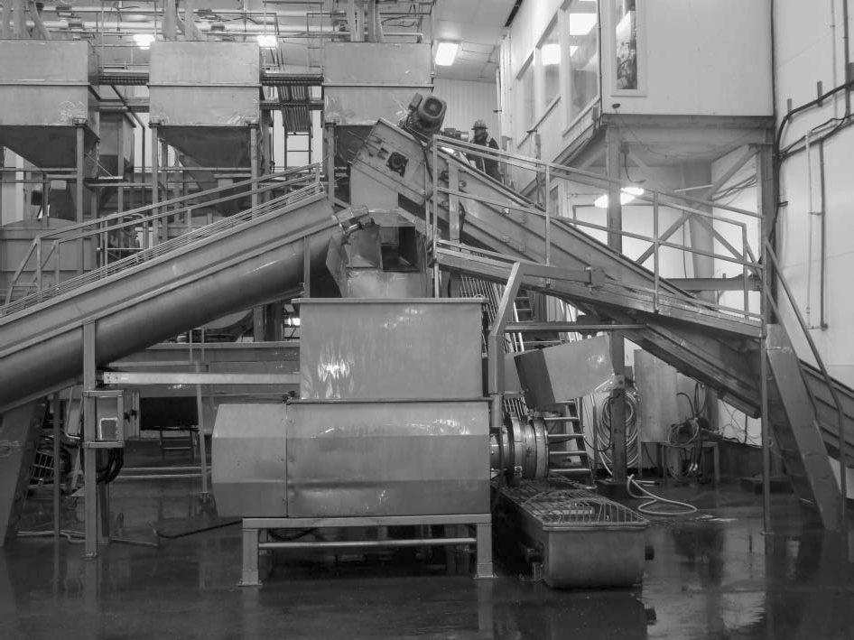
The Italian Floorlite13 example is chosen to contrast it to the Correx case. Italian Floorlite is an Italian company based in Milan; it has various plants, one of which is located in Genoa. As its name suggests, it manufactures and distributes commercial flooring and industrial rubber on the European continent. Flooring products are mostly sold to architects and designers as well as to educational, health-care, and institutional organizations. Industrial rubber is offered to companies that use it as raw material for further processing. Some components of the manufacturing process include natural rubber and natural fillers, such as clay, limestone, and dolomite.
Early in 2010, Mr. Sergio Valiantino (Ing.) was mandated with supervising the development and implementation of a new machine. This machine had never been conceived before. It had been determined that the existing production process could be cut one step. The normal workflow for the transformation of the rubber paste consisted of feeding it into conveyors where it would be squeezed between stainless steel drums, then directed along different steps to ultimately form the final sheets of rubber having various qualities (with respect to thickness, colors, coating, etc.). One step seemed superfluous; however, the rubber paste was first heated up and then cooled down, then heated up again before being cooled off one last time. What if the two heating–cooling stages were reduced to one stage only, thus speeding up the process and reducing production costs? The project to strip the process of the extra step was estimated to cost US$1.2 million.
The machine was tested in 2013 with positive results—in fact, it was discovered that the new outputs were of better quality than the ones from the old system. The machine and its production settings were achieved on time, and within budget. However, not respecting the temperature needed for the process caused the machine to jam, and cleaning it would consume a great deal of time and effort. The second “discovery” was the difficulty in training the operators. In the past, minute changes in heat levels would not lead to catastrophic results, so that employees did not have to be overly concerned with the precise handling of the various components of the machine. However, the new machine responded differently to human intervention: slight deviations of set parameters caused major problems, 100% of the time, resulting in unwanted waste and the machine locking up. Not only would this generate costs, but it would also nullify Italian Floorlite’s competitive advantage that it hoped to achieve with the new machine. The process can be exemplified in Figure 4.5.
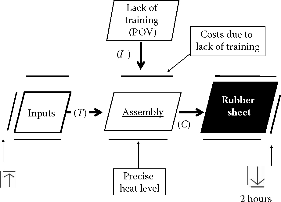
The human factor is deemed to be a negative influence. The heating of the machine, however, can be precisely set with a button, much like an oven at home. Hence, this is not a factor, but a set parameter of which management and some team members (the Forces of Production, FP) have full control—it is a minimum norm of quality. There is one POV readily identifiable: a lack of training. The problem here is not that the norms of quality are not met or that they don’t exist, but the fact that employees lack the proper training given the fact that they are accustomed to being quite lax with the temperature control as they are habituated to the old machine.
As can be seen from the Correx and Italian Floorlite examples, modeling is crucial. In the first case, humidity is a factor influencing the process—it can negatively affect the process—but the POV is undoubtedly at the entry point: the two sheets—one large and one small—must be fed into the machine at the right time. In the second case, a lack of training invites employees to be careless with the control of the heating and humidity systems, which may eventually lead the machine to jam as it becomes engulfed with overly thick or overly liquid rubber paste. Proper modeling forces the feasibility analyst and the project manager to pinpoint where, exactly, the source of a potential or real problem may be. In all cases, sooner or later, the problems will affect the calendar of activities, costs, and norms of quality or a mixture of these.
Recall that one of the main reasons for project failure is that projects are not well understood by the stakeholders (perhaps because, in part, they have different motivations, different ways of seeing the opportunity). Using a modeling system that palliates for this inconvenience is thus recommended. At a glance, everyone can see the process and figure out what is happening. The manager need not explain the sometimes-intricate working model to his employees; however, the fact that he fully comprehends it facilitates his communication. He can resort to catchy phrases and images that will work just as fine. The goal is to be understood, not to look smart.
Our basic project model is composed of three parallelograms: an input, a transformation, and an output parallelogram. But each parallelogram may be composed of a series of other submodels, with each containing its own sets of project elements (parallelograms).14 For example, the transformation parallelogram can actually be broken down into a five-project element models, which would include the vision, planning, mobilization, implementation, and the completion/evaluation stages as we have briefly seen in the previous chapter. In all, parallelograms can stand alone, and they can also exist in a series of two, three, four, five, or even more. Of course, the more project elements contained in the model, the more complex the system is and the more potential for misinterpretations to occur between stakeholders. A tip to solve this problem is to indicate that a particular parallelogram (a project element) is actually composed of a submodel by doubling its outline, as in Figure 4.6.
Processes can be examined in two ways: from a descriptive point of view (we did so when we referred to the four Ps being structural components of inputs in a project) and from an active point of view (then the four Ps are labeled Plans′, Processes′, People′, and Power′). In the case of transformation, from a purely descriptive point of view, it is expressed by the well-known life cycle consisting of the vision, planning, mobilization, deployment, and completion/evaluation stages. But we can also look at these five elements when they become active and introduce the factor time (T), which is a consequent arrow: the consequence, so to speak, of having a vision, is that eventually there will be some planning, and the consequence of planning is that there will eventually be some mobilization, and so forth.

4.3.5 Critical levels of causal bonds
Note that each type of time-related bond has a different critical level: relative time (T) can be stopped. A machine (e.g., the Correx experiment with the innovative cat litter box) can be stopped by pushing the power button or the red alert button positioned along the production line. An influence (I) can be assuaged by adopting certain measures. Suppose, for example, that the corrugated material is sensitive to the humidity level of the production and storage rooms, as can be expected; high humidity or an environment that is too dry may damage the integrity of the corrugated carton, thus making the folding process awkward and susceptible to failure. The humidity level in the rooms can be somewhat controlled with such apparatuses as dehumidifiers or their opposite: humidifiers.15 In the case of causal bonds (C), the critical linkage level is reached, and hence, carries the highest potential for POVs to cause havoc in the transformation phase. Causal bonds have no way back: once a system is put in place, it cannot be stopped. The consequent arrow will do its magic (leading to the next project element or parallelogram) no matter what. This can have dramatic results. Recall the example of the vessel in the Victor Hugo story: the loose cannon could not be stopped and it ravaged the inner gut of the vessel it was supposed to protect.
I acknowledge the fact that the PMBOK16 lists some of the consequent bonds, but not with as much detail as in my proposed methodology. Causal bonds are as follows (I complement them with my methodology):
- The start of an activity is conditional to the end of a previous activity.
This translates as the following:
• End of previous activity (C+) → start of next activity
This means that the start of the next activity cannot occur unless the previous activity has ended, 100% of the time. So we can assume that this is a causal bond, because we take for granted that the next activity is mandatorily part of the project, otherwise it would not be listed (this is, here again, a logical statement given that projects are closed dynamic systems). We also assume that we are operating along a critical path. A more precise way of stipulating this causal bond is
• Not ending the previous activity (C+) → not starting the next activity
Which reads: “Not ending the previous activity prevents the (causes the not…) starting of the next activity,” which is the most intuitive way of expressing what is happening in the process, because obviously the project planners want the first activity to take place.
In the Québec Multifunctional Amphitheatre (QMA) example, not completing the pouring of the concrete base supporting the amphitheater holds back the rest of the construction project. The same phenomenon can be expressed using C− instead of C+:
• Not ending the previous activity (C−) → start of next activity
Which reads: “Not ending the previous activity has a negative causal effect on the start of the next activity.”
The end of a current activity is conditional on the end of a previous activity. This translates as
• End of previous activity (C+) → end of current activity
Or else, in a more intuitive way:
• Not ending the previous activity (C+) → not ending the current activity
In the Mervel Farm project, suppose that a parking area is specifically allocated to the visitors of the site. Not closing the parking lot at night would indicate to would-be night adventurers or squatters that the farm site is still operating (albeit this would be a wrong assumption, but one that would fit their desires), so that they would feel free to wander on the site at night, thus possibly bothering the neighbors with loud music and heavy drinking. In other words, in order to consider the site closed for the night, the parking lot must mandatorily be locked, 100% of the time.
The start of the current activity is conditional on the start of the previous activity. This translates as
• Start of previous activity (C+) → Start of current activity
This states that, in a closed dynamic system, the start of the previous activity leads, 100% of the time, to the start of the current activity. In other words, the project manager knows that starting the previous activity goes hand in hand with beginning the current activity. In the Correx box example, the feeding of the large corrugate sheet into the folding machine necessarily indicates that the feeding of the small corrugate sheet should immediately take place, otherwise the project (the realization of the deliverable) is entirely compromised.
The end of the current activity is conditional on the start of the previous activity. This translates as
• Start of previous activity (C+) → End of current activity
In this case, the project manager knows that starting an activity will lead, 100% of the time, to the end of the next activity (put differently, the start of the previous activity leads to the end of the current activity). In other words, the first activity is not technically completed until the end of the second activity has occurred. For example, the mobilization of resources serves no purpose if they are not put to use in the next stage of the production process. Within the transformation phase of the project, the mobilization stage has a causal effect on the completion of the implementation stage (given a closed dynamic system); otherwise, the entire effort is a lamentable loss. The reader can thus see that, under pressure to complete the project, the implementation stage will continue affecting the mobilization stage if resources fall short. This can cause delays and increase costs. Thus, this particular setting betrays lurking POVs.
We can estimate the critical level of POVs of these scenarios as shown in Table 4.3—keeping in mind that the more the project runs along a critical path (and gets closer to the due date of delivery), the more critical the level is.
| Type of causal link | Critical level of POVs |
|---|---|
| Not ending the previous activity(C+) → not starting the next activity | Low because no costs are associated with the next activity |
| Not ending the previous activity(C+) → not ending the current activity | Moderate because both activities are assumed to be near their end |
| Starting the previous activity(C+) → starting the current activity | Serious because the process will not work unless both activities (which both incur costs) are given the go-ahead |
| Starting the previous activity(C+) → ending the current activity | Critical because there is intense pressure once the entire process has begun |
The project feasibility expert would be well advised to identify T and I bonds, and to specify the types of causal (C) bonds that exist in the process he is examining, because all of these bonds attract different critical levels of POVs.
What this effort does is help specify the location of potential POVs. Indeed, the causal link is often an indication of a potential POV. If the activities are relatively inconsequential, then the causal relationship may be dealt with at some point during the project; however, causal links along the critical path are undeniable expressions of potential POVs. If one element of the process drifts, then automatically, the other fails too, altering the course of the critical path ascribed to the project. Hence, assessing causal links in the context of critical paths is one way of unveiling POVs.
Let us take the example of the Montréal Olympic Stadium (MOS). The start of the 1976 Games was conditional on the completion of the main infrastructure; namely, on the functional completion of the stadium (it had not been completed as per plan, but it would be functional). Hence, we have the following:
- End of previous activity (C+) → start of next activity
Alternatively, we have
- Functional completion of the stadium (C+) → opening of the Games
This is a causal link in the sense that the Games could not take place until the stadium was functionally completed; there was just no way around it. Putting it in the context of a critical path gives us the following:
- Functional completion of the stadium prior to July 17, 1976 (C+) → opening of the Games on July 17, 1976.
In fact, to be more precise, we have
- Incomplete functional completion of the stadium prior to July 17, 1976 (C+) → no opening of the Games on July 17, 1976.
This expresses the conditional aspect of the causal bond. It also shows that there is a POV: the project would not be completed unless the stadium was functional prior to July 17, 1976. The feasibility analyst could then look back and try to identify everything that could prevent such activity (the functional completion of the stadium) from taking place.
We have thus added to the meaning of the PMBOK a proposed list of causal bonds. The reader can see how the methodology suggested in this book goes one step further than the PMBOK and other such books on project management and how it helps uncover POVs. With this last example, the reader can also appreciate how important it is to conceive a proper model of the project.
The influence (I) bond should also be understood in all of its peculiarities. There are two kinds of influence: direct and indirect. The direct influence (which can be I+ or I−), directly affects a process element (a parallelogram) as in the case of humidity affecting the cardboard in the Correx example. Indirect influences affect process elements in two ways: mediating or moderating. With the mediating way (which can be I+ or I−), a process element is introduced between two existing process elements to offer an additional route to the straight line process between these two process elements (parallelograms). With the moderating way (I±), a process element can influence the interaction between two existing process elements in one of two ways, depending on the point of view or on circumstances: either positively or negatively, hence the code (I±). There exist statistical methods to identify mediating and moderating variables (process elements), which I will briefly discuss in the chapter on People. Table 4.4 illustrates the different types of influence bonds.

Some production processes are designed in a way that there is a contingency provision: should one line of production slow down, an alternate route channels the production units that will eventually land on the output deck, where they will be collected for storage. This is a mediating process. It occurs in the brain as well: some neuronal paths are networked in such a way that if a flow of information cannot make it, say, from point A in the brain to point B in the brain (e.g., because of delays or damage), then an optional route is offered that sees the flow of information going from point A in the brain to point Z in the brain, and then to point B in the brain. Point Z is a temporary node through which the information flow travels in order to move from point A to point B. Often, point Z presents a certain number of advantages: it allows the route A–B to catch up on delays, for example, or to upgrade the quality of information because point Z contains bits of data that can enrich the information that is traveling.17
In a project, it is most useful to identify mediating routes because they help reduce the dangers associated with POVs. If something goes wrong with a particular process, then an alternative path can be used. At times, paths A–B and A–Z–B are engaged concurrently at different levels of usage. This softens the otherwise uncompromising level of the critical path. In short, POVs on critical paths are more dangerous than POVs on paths where mediating options exist. Mediating paths are often designed when preparing contingency plans, by posing the question: “If this does not work, what other option can be put in place?” An example is the emergency staircases in high-rise buildings: if elevators cannot be used to go from, say, floor 12 (point A) to ground level (point B), what alternative can be offered? Well, a staircase going from floor 12 to floor 5 (point Z), where occupants of the building must stop and go to another set of stairs to go from floor 5 to the ground floor. This ameliorates the security of the entire building because it cuts into the possibility of flames engulfing the entire exit path (what would have been a single stairway). Note that mediating paths are diagonal flows in the sense that they take a course off of the straight direct flow; when the unit that is being processed travels along the mediating flow, it is often improved. As such, the deliverable is not exactly what was predicted, an observation that meets the definition of a diagonal flow.
Point Z (floor 5) palliates for the POV that a single staircase represents in such a context. Note that we are still dealing with consequent arrows and parallelograms, that is, with processes. Time is therefore a factor. Indeed, in this case, if it takes too long to go from one set of stairs to another one on floor 5, the entire reason for having set such an emergency pathway is lost: smoke and flames will catch up before the occupants can escape. Time is of the essence in modeling with consequent arrows.
It can be added that POVs weaken any process system: they work against it and thus form a negative force, which the four Ps should theoretically combat. POVs have two ways of exercising this negative force, by way of (1) excesses (e.g., excess procedures dragging the production process) and (2) shortages, acting as a hole in the process (e.g., insufficient information or a shortage of material). In both instances, the process draws to a halt or else moves backward, which is contrary to the objective of the project.
As for moderating influences, generally these factors affect a process one way or the other. On some occasions, these factors can be beneficial, on others, detrimental. This is why the symbol (I±) is used. Often, people (such as scientists) argue because they treat the same process without realizing that the factor affecting it can have an opposite influence depending on circumstances. People then quarrel bitterly over the same thing, occasionally with frowns and menacing stares…uselessly! This aggravates conflicts and misunderstandings. This is why it is so important (I emphasize this again) to resort to proper modeling when preparing the plan for the project.
The use of an external consultant in a project serves as a prime example. Some of the employees will react favorably by recognizing his value, and will therefore cooperate. Others will feel threatened—fearing, for example, that they may lose their jobs—and hence will become defensive, if not unfriendly altogether. This is true in the case of a team of experts in human relations (HR) that is invited to come and hone the skills of an existing project team. Some project members may actually believe that the experts have been hired not to improve their work conditions, but to find a way of laying them off. The experts—characterized here as a process element—have an antagonistic position: they appear good or bad, depending on how one looks at them, and probably on circumstances (the project goes well versus the project experiences difficulties). It is easy to see that moderating process elements can serve as a catalyst to awaking dormant POVs.
Overall, we have what is displayed in Table 4.5.
When the two elements being linked by a bond move in the same direction (when one goes up, the other goes up, or ↑ ↑), a positive sign is employed (e.g., I+); when they move in the opposite direction (↑ ↓), a negative sign is used (e.g., I−).

So far, I have examined consequent arrows: what they have in common is that they cannot occur without the passage of time. All project-related processes fall within one of the three types of consequent arrows: longitudinal (T), influential (I), or causal (C). Ideally, the project feasibility analyst should be able to draw up each and every process by identifying the type of arrows that are pertinent between the various process elements.* Recall that a Dominant strategy is achieved when the project manager can control the project, that is, in the present context, when he can verify that all processes (parallelograms and arrows) work according to plan. On the contrary, a Short strategy is implemented in a hurry when the project manager reacts to unforeseen events. Without a doubt, a Dominant strategy has greater chances of being achieved when a proper plan is set, that is, when all processes are captured and analyzed using parallelograms and T, C, and I bonds.
Let us revert to the Mervel Farm example. From a macroscopic point of view, the inputs are Plans, Processes, People, and Power. With time, these inputs enter the next process element (parallelogram): transformation. Within this phase, all four Ps interact with each other (to become Plans′, Processes′, People′, and Power′) and various influences could actually affect this phase. Finally, with time, some deliverables (as well as some form of knowledge and impacts) are generated: the opening of the summer trail for the first Pierreville-based agricenter. This is a longitudinal process. Let’s focus now on the input phase and assume that if no government funding is available, then the project will not go ahead despite the fact that it is deemed feasible from a technical point of view. Hence, we can express this by saying that the start of the next stage (the opening day) is conditional to the end of the previous activity (funding). It could also be possible that the project would go ahead without funding being available because the promoters believe that they could eventually collect the money that they need. In the latter case, the start of the next activity (the opening day) is conditional on the start of the previous activity (some funding). We can express the first scenario as the following: if there is no full funding right up front, then there is no opening day. End of previous activity (complete funding) (C+) → start of next activity (grand opening). Indeed, the government would not grant money if it was not absolutely convinced that the project could materialize. There is a potential risk: what if the money is misused? What if the government postpones granting the money because it is an election year and the dollars could help gain more votes thanks to another project? The presence of an election campaign acts as a moderator for the input phase: it could be good and it could be bad for the project (I±)—nobody knows the results of the election yet. Assume that the promoters have conducted a marketing study and found that the project is vouched for by most citizens. That’s a positive influence (I+). But it may be the case that citizens living close to the farm fear the flow of traffic, the farm odors, and the noise. Their opinions and actions would exert a negative pressure on the project (I−). Now, assume the project is set to take place across the entire Mervel Farm land and that a provision is secured to set part of the summer event in a nearby park in case the flow of traffic becomes too big to handle. That’s a mediating path: an indirect positive influence. Let’s now look at the transformation phase. Its parallelogram would be designed with a double outline, to indicate that there are one or more submodels associated with it. The first submodel would be the five stages of transformation typically found in a project life cycle: vision, planning, mobilization, implementation, and completion/evaluation. Say we take mobilization. This process element (parallelogram) could also be composed of different process elements linked together by T, C, and I bonds.
By applying the same strict logic across the entire project definition, the feasibility analyst minimizes the chances of errors; we could even venture to say that improper modeling is a POV in itself. If it weren’t, there would be no issues with team members fretting about not respecting the plan, not understanding the project, not fulfilling the work tasks, and not delivering.
Our analytical foray does not end with consequent arrows. We must now address descriptive arrows, which come in two types: structural (they can be “binary” or “continuous”) or functional (generally measured on a continuous scale).18 The reader has actually already been exposed to both of them. The four Ps are structural (descriptive) process elements linked to inputs by structural (descriptive) arrows. Deliverables, the book of knowledge (BOK), and impacts are functional process elements linked to outputs by functional arrows. Descriptive (structural or functional) arrows are not related to time. Time is absolutely not to be taken into account. In the field of statistics, some authors19 set the following conditions for formative variables, which I apply to my concept of structural variables: (1) changing or withdrawing one variable alters the meaning of the core concept and (2) there should be little or no colinearity between the structural variables. Along these lines, it has been said that “omitting an indicator is omitting a part of the construct.”20
The code for visualizing a structural arrow is as follows: at least two process elements are required to be linked by way of arrows to one single process element (parallelogram). If it weren’t the case, the one structural element would simply equal the second structural element, making it superfluous from a modeling point of view. Also, each arrow leaving the structural process element to reach the single main structural element must head for the same single point on the parallelogram that represents it. Let’s take the four Ps. The first condition is met: there are at least two elements pointing toward the main process element—inputs. The second condition is that each of the four Ps in the parallelogram points toward the same point on the parallelogram representing the main element—inputs. This is one sure graphical way of differentiating between consequent and descriptive arrows.
There is more. The four Ps represent essential conditions defining the main element—“inputs” in this case. All structural elements forming a main structural element must be sine qua non conditions. The main element—inputs—is not fully defined if any of the four Ps are missing. The four Ps form the parallelogram of inputs. One can think of it this way: A bicycle is mandatorily formed of a seat, pedals, a frame, two wheels, and so on. If it consists of one wheel only, it is no longer a bicycle but a unicycle. If it is composed of three wheels, it is a tricycle, not a bicycle. Without a doubt, the two wheels, along with the seat, frame (etc.) form the “bicycle”. Again, this is tantamount to formative variables in statistics.21 The key point for the feasibility analyst is that he must learn to find all the elements that are sine qua non conditions for forming the main process element. For example, in the case of the Correx process, because there are two corrugated sheets that need to be brought and glued together, a sine qua non condition to the machine that will be built to produce the innovative cat litter is one that obligatorily has two entry feeding points: one for the large corrugated sheet, and one for the small sheet. Hence, everyone can realize that the machine will not produce what it is supposed to produce—the innovative cat litter tray—if it does not have two mechanisms permitting each of the corrugated sheets to reach the main conveyor.
To identify the structural components of a process, two questions must be posed. First, returning to the bicycle example, the feasibility analyst would ask: “Is a seat a necessary element to define a normal bicycle?” If yes, it is a step toward determining that it is a structural element. “Are two wheels necessary to build a bi-cycle?” The answer being “Yes,” the two wheels are most likely structural elements of the main element—the bicycle. The feasibility analyst has to go through every possible scenario in order to fully define the main process element; failing that, he will open the door to POVs. Indeed, if brakes are missing on the bicycle (thus making the main element—the bicycle—incomplete), the project of riding a bicycle becomes dangerous and the child riding it is in a precarious (vulnerable) position. Not having determined that a normal bike is composed of brakes has led to creating a POV with potentially disastrous effects. The second question that must be posed is the following: “Do the handles exist independently from, say, the seat?” If the answer is “Yes” then that’s an indication that it is a structural element. “Do the handles exist independently from the frame?” “Yes.” All permutations between each potential structural element must be checked in order to confirm that there is no colinearity (no correlation) between them. If there is, then the potential structural element is not a structural element, but a functional process element.22
The reader should be aware of the impact of the absence of colinearity. In a statistical sense, it means that a regression can be run without having to pay attention to the interaction between each of its variables (with functional elements, there is colinearity, thus making regression analyses much more complex). This can be expressed as follows23:
Where the Xs represent each subelement (a process element that forms the main process element, such as the handles and brakes) and β the level of influence of the respective subelement on the main element. The analyst need not worry about possible interactions between each X because there is none; this is a condition for establishing that the X is a structural element of the main element. In this case, there is no room for diagonal processes; everything is straight direct.
In the examples given so far, each P of the four Ps that is present at the pretransformation phase is completely independent of the other, and each is a sine qua non condition for structuring “inputs”. Similarly, I have defined People as being composed of customers, suppliers, regulators, and bad apples. I speculate that bad apples are a necessary part of the equation forming People. Customers can exist independently of suppliers (but will not buy anything) and independently of regulators and bad apples, and there can be no People on a project without customers. So “customers” is a structural element defining People. However, it takes at least two structural process elements to form another one, so that if I had only first identified customers as forming People, I would have obligatorily sought to find at least another element (in fact, we outlined three more—suppliers, regulators, and bad apples). This way of thinking ensures that each and every time, the feasibility analyst fully clarifies the parts of the project that is evaluated.
This analytical method is a great way of uncovering POVs because these develop most often when there has been a lack of definition: POVs grow like mushrooms, in dark and humid conditions! Again, a project that is well conceived is a project that can hardly go awry. The advantage of this method is that it helps in the modeling of the project because generally, process elements tend to be symmetrical. If there is an off button, there is also an on button. With respect to the brain, the same process occurs: there are molecules in the brain (neurotransmitters) that facilitate the emergence of certain behaviors and others that inhibit them. In cats, for example, hostile predatory behaviors cannot exist at the same time that defensive behaviors take place. That’s because the neurotransmitters that act between three of the brain areas implicated in the mechanics of the behavioral response (the central amygdala, the lateral/medial hypothalamus and the periaqueductal gray area, or PAG) are either activated or inhibited, but never concurrently. When the medial hypothalamus is activated, the lateral hypothalamus (responsible for Instrumentally hostile aggression) is inhibited. We will see this further in the chapters on People (Chapters 5 and 6) and Power (Chapter 7). The point here is that proper modeling tends to generate symmetrical patterns, which greatly helps understanding processes.
One last note on structural process elements: they can be measured in two ways, which I call “binary” or “continuous”.24 A binary structural element is one that is measured by posing the simple question: “Is it present, yes (value = 1) or no (value = 0)?25” A so-called continuous structural process element is measured by a scale where a range of values greater than 2 can be used. For example, a scale of 11 alternatives could be used, with 0 not being offensive at all and 10 being critically offensive. Binary scales associated with a structural arrow are marked (Sb) and continuous scales associated with a structural arrow are marked (Sc). This allows the analyst to quickly establish what kind of measurement is favored for the structural elements pertaining to the project process under review. Refer to26,27 Figure 4.7.

In Figure 4.7, I look at the resources and Means of Production from a descriptive point of view: they are sine qua non variables elected to define Processes. There can be no process to speak of without the resources and the Means of Production. In the last example, the analyst has chosen to measure resources with a yes/no question (are resources available “Yes” or “No”; he is using a binary measure). However, he has established a continuous scale for Means of Production, so that he may be operating on a question like: “Are all Means of Production prepped to enter the transformation phase?” Also, since the analyst has decided to look at transformation from an active point of view and not from a descriptive point of view, the four Ps exert an influence; they are no longer structural elements (truly, they are structural variables forming “inputs”, but “inputs” by itself is not an active concept).
During the vision stage of a project, it may be possible that the promoter is not entirely certain of what characterizes the project in all its details. There will come a point when he will be required to determine all of these details, but in the meantime there is room for flexibility. To account for this, a small s can be used: (sb) for a binary structural element, and (sc) for a continuous structural element. In accordance with the format system adopted in the present methodology, these codes appear graphically on the bond linking two parallelograms. This way, the nature of the bond is specified: it is a structural bond, a tentative one, and it is measured with a binary or a continuous scale. As the reader can appreciate, working this way provides plentiful information that can be used to get a limpid picture of the project processes and to reach prompt and precise decisions.
With structural process elements, we speak of sine qua non conditions. This is not the case with functional process elements. Structural elements explain what the main element is mandatorily made of. Missing the inclusion of one of the necessary components (elements, which can be material items, abstract concepts such as “People”, or processes in themselves) means missing the opportunity to fully define the main reference element. Imagine sending a man to the moon without reserves of oxygen. Oxygen is an essential input for the space shuttle, 100% of the time. Functional elements do not refer to what the main process element is mandatorily made of, but rather to how it functions. Let us take the example of the bicycle yet again. Suppose the reader does not know what I am referring to. However, I indicate that the object I have in mind is a key element of the Tour de France, that it does not use gas, that the maximum speed it can safely achieve in a downhill is 44 miles/h (70 km/h), and that it uses man (leg) power. At this game of charades, based on pure functionality, most readers would have guessed that I am referring to a bicycle and not a turbojet. A tricycle cannot achieve a speed of 44 miles/h. A car cannot be moved solely by manpower. So the object that I have in mind is, probably, in fact most probably, a bicycle. The more the functionality of the mysterious object is detailed, the more convinced the reader will be that I am talking about a bicycle. So the reader has managed to identify the object (or the process element) without mention of any one of its structural elements (pedals, wheels, etc.). This means that all process elements can and must be established in two ways: structurally (S) and functionally (F).
Note that the functional aspect of objects is regularly utilized in science. For example, scientists can infer the presence of a planet without ever seeing it simply based on how surrounding planets and suns behave.
Recall that quality was defined as [(Functionality + Design) over Costs]. If we equate functionality with functional variables and design with structural variables, we thus obtain this meliorated version of perceived value definition:
Logically, if the feasibility analyst wants to determine the quality of a project, he must identify and quantify its structural and functional process elements. Hence, there is no way around properly conceiving a project; most people, anyway, behave in a way as to maximize their value (in financial terms: their wealth). By highlighting the value of the project to the team members (Forces of Production) who participate in it, managers get them even more motivated and dedicated, thus reducing the potential effects of stealthy POVs.
A functional description is coded (F) and can be measured in a binary or, more usually, in a continuous way (Fb or Fc). Functional elements are not sine qua non conditions. For example, one could progress without the reference to the Tour de France and eventually guess that the object that is under investigation is a bicycle. It helps to know that it has something to do with the Tour de France, but the fact is that it does not preclude the identification of the object. The more pertinent key functional characteristics that are enumerated, the closer we get to unveiling the mysterious object. Furthermore, functional elements interact with each other—they contain some levels of colinearity. Recall that the output portion of our project definition model has been linked to deliverables, formalized knowledge, and impacts. If the reader goes back to Figure 1.3, he will see that the arrows start from the same point on the parallelogram identifying “outputs” and point toward each of these three items. This is an indication that time is not a factor and that we are dealing here with functional elements. There would be no impacts if there weren’t any deliverables; deliverables and impacts have some form of colinearity. There would be no useful formalized knowledge if there were no deliverables. There would be no useful formalized knowledge if impacts, both positive and negative, were not discussed. As can be seen, functional elements have some kind of relationship between them, which makes running multiple linear regressions a challenge because the interactions must be taken into account—doing otherwise is reducing the meaning of the linear regression. Another point is that there can be any useful number of functional elements, yet at least two are necessary, just as was the case with structural elements. But taking one functional element out of a list of 10 does not diminish the functionality of the main element; a contrario, taking one element out of a list of structural elements is very damaging to the meaning of the main process element. Functional elements are akin to reflective variables in statistics.28
Let us take some examples. The cat litter box can actually have multiple functions: it certainly can be used as a cat litter box, but it can also serve when fruit picking at the Mervel Farm, or as a gift container at the gift shop located at the same farm. Should it be used as a cat litter box, there is little justification for paying extra money to decorate it with fancy colors—most cat litter boxes are kept in a dark laundry room hoping the unpleasant odors will not reach the living room or the kitchen. However, if it were used as a gift basket of sorts, then a colorful print on the otherwise dull brown cardboard could be an asset in order to sell the product. So, functionality has in some way defined the process element that has been produced out of two flat, glued-together corrugated sheets. Similarly, there are projects that have very little impact to speak of, and others that don’t really generate formalized knowledge; yet, the fact that they do would be somewhat of an indication of the size of the project (and probably of its costs) without ever knowing what projects are referred to.29 The same thinking process occurs in a criminal investigation or archeology, or even geology for that matter. Finding a 2000-year-old skeleton with a sharp wound on its shoulder blade and a nearby small triangular stone that is obviously man-made may be a hint that the individual was the victim of an aggressor while he was running for safety (he was obviously hit from behind). The functional elements (e.g., the triangular stone is part of a tool utilized for hunting) help generate a scenario of what likely happened.30 Thus, identifying the functional process elements of a main process is a very handy way of tracking back errors that have disabled a project, or else of anticipating POVs (the victim’s back in this case).
Let us accept the fact that the functional elements of the Québec Multifunctional Amphitheatre (QMA) are (1) a venue for entertainment and (2) a sports center (more specifically, an arena built in the hope that the city will soon be awarded an NHL team franchise, which it once had in the 1980s with great success31). The two main functions of the QMA are set. Suppose the ice rink does not work. Then the reason for being of the QMA (the main process element being the QMA) is amputated by 50%. In other words, failure is knocking at the door. The process of analyzing the fact that some of the functional elements of the QMA have been amputated can start by going back along the parallelograms and arrows that have been part of the entire model, including S and F, T, I, and C arrows. In short, all project management processes can be pictured by way of two kinds of descriptive arrows (S and F) and three sorts of functional arrows (T, I, and C). In reality, the S and F arrows fall under one heading: descriptive. S and F are both used to describe a process element. That’s all there is to it. The science of physics is entitled to its four forces (weak bond, strong bond, electromagnetism, and gravity), so why would project management not have its own four forces as well: descriptive, longitudinal, influence, and causal?!
A chessboard holds 32 pieces—16 white and 16 black. Each piece has its own operating mode. The pieces interact with each other once the clock starts ticking. Billions of patterns exist (an estimate is that 10120 games are possible32), yet good players can play back their games from memory. Why? Because they have followed a certain logic that can be expressed by S and F, T, I, and C codes. Knowing the S and F of each piece, there are moves that can influence the opponent action (e.g., what is referred to as a “pin” in chess), moves that lead the other player to use time to prepare his response (certain moves in chess are made only to confuse the opponent and force him to exhaust valuable time), and other moves that can cause the opponent’s actions (so-called forced moves, with the ultimate forced move being the throwing of the desolate king against the wall angrily, or more diplomatically, accepting the loss). There are just no other kinds of moves given the S and F nature of the chess pieces. When a chess player remembers a game, he usually tries to reason as to why the pieces on the chessboard are located where they stand; he then examines his motivation (to delay the opponent’s response, influence a move, or force a move?). The most dramatic situation and the one that the player tries to optimize is one where he forces a move from the opponent. Throughout the game, as previously mentioned, the chess player engages preferably in a Dominant strategy or else in a Contingency strategy, depending on the context; yet whatever the positional strategy, S and F, T, I, and C explain every move he makes. Victory is in sight when the player has defeated all odds of losing (of being attacked on his/her POVs) or of coming to a draw, and similarly, success in a project is ensured when a project manager has defeated all odds of POVs becoming active.
Again, each and every process is fully comprehended from a descriptive point of view by way of identifying structural process elements and from a functional point of view by way of listing relevant functional process elements, nothing less. Both sides (structural and functional) of the object (process) must be assessed, otherwise the object (process) is deemed to be poorly defined. And, as mentioned from the start, a poor plan leads to derailment. Refer to Table 4.6.
Recall that I have resorted to walls, ceilings, and floors when discussing some processes in the introduction of this book. Let us take the example of the humidity factor as a negative influence (I−) in the Correx cat litter process. Under normal conditions (which have to be assumed in a production plant), humidity levels can reach a certain minimum and a certain maximum level, which will influence the cardboard behavior along the production line, without compromising the process. In the case of the Italian Floorlite’s rubber sheets, minute changes in temperature levels during the heating process can cause havoc. The minimums and maximums are so sensitive that they escape the normality of the production conditions. Hence, in the end, not having respected the quality floor (the norm of quality) causes the production line to peter out, as it becomes jammed with a thick paste or else filled with an excessively liquid paste that quickly penetrates all the mechanical parts of the machine. Establishing walls, ceilings, and floors along the parallelograms (process elements) is just as critical as specifying the types of bonds that exist between them.
| Type | Avoid | Code |
|---|---|---|
| Structural (S) | Doing a regression without independently measuring the main construct | Binary (Sb) Continuous (Sc) Temporary (sb or sc) |
| Boosting Cronbach’s alpha66 | ||
| Functional (F) | Not recognizing colinearity | Binary (Fb) or Continuous (Fc) |
To prove my point that modeling is critical to any feasibility study and that levels expressed by walls, ceilings, and floors are a crucial consideration, I follow with a real case involving the use of my modeling technique in a wildlife context.
4.3.6 Example taken from wildlife
In 1972, the United Nations published the Atlas of the Living Resources of the Seas, which provided a map of the marine areas where fishing was encouraged (I+).
Over the years, however, the coastal areas of the oceans have literally turned into a gigantic soup of jellyfish. Recently, a Swedish nuclear power plant was put out of action by the presence of these marine animals, which had clogged the cooling filters of one of the reactors.33 Jellyfish are inexhaustible zooplankton predators, but do not represent much nutritional value for most predators (such as tuna and turtles), being composed of more than 90% water.
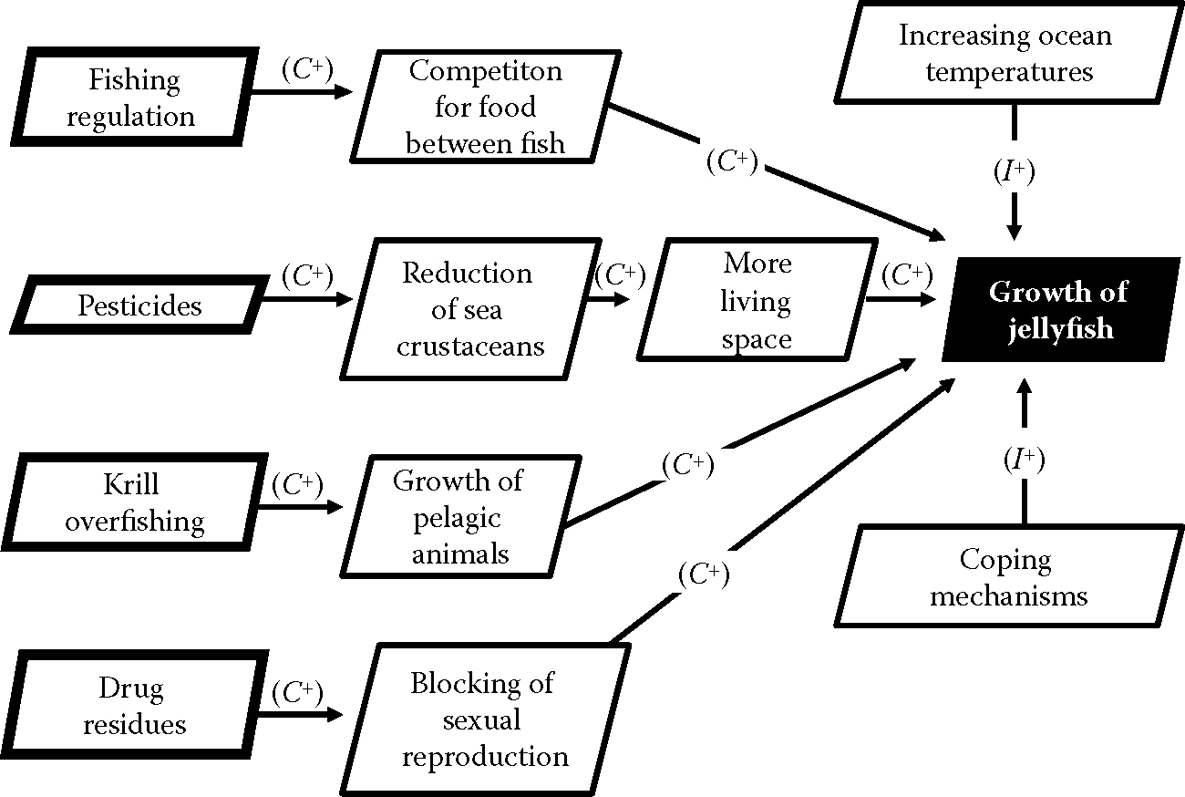
The causes of and influences on the proliferation of jellyfish are multiple. Overfishing has left a vacuum by fostering an opportunity for jellyfish (cause C+) to expand because the competition from fish for the same food sources has been augmented (cause C+) as resources becomes scarce. Increased ocean temperatures have facilitated (influence, I+) the population growth of jellyfish. These have now supplanted fish in the food chain in many marine regions. Krill overfishing has also worsened the situation (cause C+): their relative absence has allowed pelagic animals, known for high rates of growth and multiplication, to occupy a larger portion of the ecosystem (cause C+). Furthermore, toxic products associated with pesticides employed in modern agriculture that end up in the sea have been found to block the growth of sea crustaceans (cause C+), so that there is less food for fish and more living space for Salpae and other gelatinous organisms (cause C+). Also, drug residues discharged into the sea by way of sewers (containing urine) act as endocrine disruptors (influence I+) that block the reproduction of sexual species (cause C+), but not that of jellyfish, which use an asexual budding reproduction system (poor guys, they don’t know what they’re missing!). Finally, jellyfish have developed coping mechanisms (such as the ability for some to regress to an earlier stage of development) so that their level of vulnerability is minimized at the end (influence I+).
In short, fisheries’ policies or the way they were implemented have maximized the vulnerability of certain species of fish through a series of causes and influences (for which we have just made a judgmental evaluation), while it has reinforced the survival capacity of jellyfish, an animal that has gone through 600 million years of evolution.
This process can be exhibited as shown in Figure 4.8.
Recall that there should be only one point of entry, so that the model in Figure 4.8 is only partly true. When we look at it, the problem is not fishing regulation per se, but the lack of proper regulations for fishing krill, as well as pesticides and drug disposal. Hence, the entry point is a “lack of proper regulation”, which is then expressed by four process elements (functional variables): drug residue disposal, fishing regulation, krill overfishing, and pesticide management. Hence, using this methodology, we get a better picture of what is leading to the explosive population growth of jellyfish.
If we transpose this entire process in a project context, the picture of the situation is crystal clear thanks to efficient modeling. In addition, the reader can appreciate the importance of determining POVs in advance, because the consequences can be catastrophic in a closed dynamic system such as the marine system or any project. In the jellyfish example, nature has it that they have developed coping mechanisms to deal with their own POVs, which has then assisted them with their survival and expansion.
Note how judgmental it can be to draw a model sometimes, such as the aforementioned marine process. Some experts could contend, for example, that overfishing is not a cause, but simply an influence.
The explanatory powers of each of the four fundamental types of bonds (descriptive, S and F; longitudinal, T or t; influential, I; and causal, C) are not equal. A project manager would not be well received by saying that his assignment had turned into a muddy outcome because that’s just the way the project was from the get-go (descriptive). I assign a value of zero in terms of the explanatory power of this approach. An expert could claim that the growth of the jellyfish population happens with the passage of time, which is true, but which holds very little explanatory power (let’s assume an explanatory power of 0.5). They could claim that there have been factors that, when they increase (↑), are accompanied by a surge in the population of jellyfish (↑); this only goes as far as explaining why the ecosystem is changing, but does not provide the reason for why it is changing in one direction (increasing jellyfish population ↑). We ascribe a value of 0.5 as an explanatory power to this statement. The same scientist could vehemently contend that overfishing is the root cause (C+) of the jellyfish population explosion, but knowing that there are other variables, such as the presence of endocrine disruptors, makes this statement questionable: if proved wrong, the scientist’s reputation would be tarnished. He may be 50% of the time wrong or 50% of the time right; nobody knows for sure yet. We cannot attribute a value of 1 to this presumed causal link, but must rather settle for a value of 0.5 because of the probability that the scientist may be wrong, given that causal links are generally very hard to prove.
If we are project managers who have to explain why our project has not achieved its goals, we’d like to leave all opportunities to justify ourselves while finding the safest stand. By saying that we think there has been a link between what was done and what was achieved, but by leaving the door open to the presence of negative factors, I–, that may be to blame, or else by claiming that time is the culprit, or else that a possible cause should not be discarded, we are sort of mitigating our damages—we can hardly be accused of not considering all options. Many scientific reports are concocted that way, and even when a causal bond is suspected, a scientist will find a way of questioning it. The example of the tobacco industry speaks volumes: some scientists are convinced that there is a causal link between cigarette smoking and lung cancer, while others say there is no sound evidence of such a causal effect and claim that the causal argument is, well, smoke and mirrors! Most people would agree, however, that there is a link between one and the emergence of the other.
Modeling implies a trade-off between what is certain and what is uncertain. Models are not perfect, they are a simplification of reality. The lesson learned here is that when it comes to project management processes, looking at bonds while acknowledging all of the options that could explain the project difficulties is a sharp way of approaching things, keeping in mind how these options ignite POVs.
4.4 Modeling language
As the reader can judge, I have developed a language specifically for the purpose of conducting project feasibility analysis. The basis of it is that all processes must be brought to their ultimate causal (C) condition, nothing less. It is only by doing so that the expert can see where POVs lie. To achieve this, we avoid completely any routes of escape, such as “if this, then that,” “either (…) or,” and so forth. Every process must be straight direct. The point here is not necessarily to write an entire production process into this language but rather to use it as a tool to better circumvent a particular process and see what could go wrong.
To show how the modeling language works, let’s take another real example, that of Bleu lavande (“Blue lavender”). The reader will realize that the language I develop here explains a lot about human behavior as we shall see: most people, consciously or not, bring events to their critical path, that is, to their causal dynamics. It is often because of this critical causal thinking that people tend to disagree with each other or lack proper diligence, resulting in poor processes.
4.4.1 An example: Bleu lavande
Bleu lavande34 is a medium-sized company based in the Eastern Townships in Québec, Canada, an area known for its kaleidoscope of vibrant colors in the fall, with festive orange, red, and beige hues spreading over acres after acres.
An entrepreneur cautiously chose the location to start a unique business after much research: growing lavender and transforming it into lavender-based products such as essential bath oils, hand sanitizers, and so forth. Lavender was not a traditional plant in Québec, although it had long been a landmark product in France. The fields where the plant grows have to be slightly inclined and there has to be enough sunlight. The business developed nicely, but a strategic miscalculation led it to bankruptcy even though demand was high and the market kept expanding. Instead of using existing specialty stores across the province to sell his products, the entrepreneur established his own stores. But there is a wide margin in the kinds of operations that are entailed in the retail business and farm-based operations.
The business was salvaged and has been successfully operating since 2015. In the summertime, agritourism provides an important source of revenue: the fields as well as the farmhouses and transformation operations (steam distillation) are open to the public, who line up and pay C$10 to access them. The neat thing about the concept is that anyone can actually see how the outputs—condensed lavender oil and its by-product (a near transparent liquid that smells something like lemon, but with a rancid undertone)—are manufactured.
I endeavor here to write the entire process using our modeling language technique to show how POVs can be identified.
First, the seeds are planted in the soil. A concern is to avoid contamination by a plant that emulates almost perfectly the lavender flower and branches, but which produces poor quality oil. Let us start at the point where the plant must be harvested: late in July.
- Lavender plant (T) → harvested
The word “harvested” is underlined because it is an operation. Time is the kind of arrow that takes place because the lavender plant does not influence (I) the transformation process, it does not define (S and F) this transformation process, and certainly the plant itself does not force (C) the business owners to process it. A day late in harvesting would not make a significant difference.
There are three worries during that first step: time, costs, and norms of quality. Only time is a real factor: not harvesting during the critical harvesting season means losing the quality branches and flowers required for transformation. Hence we have
 Lavender plant (T) → harvested
Here, we must have an entry wall. Walls refer to time (T). There is no loop (t) as the plant, once picked, cannot be put right back into the soil. Now, we want to turn this into a critical path because that’s how we spot POVs. We assume that the plant loses its essential quality past August 20, and so that is the absolute deadline. We have the following:
- July 1, Lavender plant (T) → harvested, August 20
- August 21, Lavender plant (C+) → poor quality, June 30

Therefore, the causal link occurs within these boundaries—August 21 to June 30 of the following year. We assume that all plants have been transformed and sold by June 30 of the following year, so that the end wall is nearly a year after first harvesting. The question that comes next relates to transformation. We know that transformation is the act of management, and where the team members (the Forces of Production, FP, both controlled and uncontrolled) use Means of Production, MP (e.g., land/building, machinery/equipment), to transform inputs into outputs. POVs must therefore be found in FP, MP, or inputs. Note that weather conditions are not a POV, they represent an external risk. The question is: “What are the chances that the FP will miss the entry point of July 1 and the deadline for harvesting of August 20?” For this to happen, there would have to be a strike or a dramatic shortage of labor; in either case, the producer could palliate the problem by hiring local farmers and students. The POV is weak. There could also be a break in the tractors used to collect the plant: this is a more serious predicament. This entails the following:
- Poor MP (C+) → slow (or delayed) harvesting
Slow harvesting would lead to delays and bring the harvest past August 20, so that the process would enter into a critical (POV) zone. So, looking at this process sentence [Poor MP (C+) → slow harvesting], we immediately seize the importance of checking the machinery before the harvesting season starts.
Finally, the last elements of the inputs are resources (such as electricity, gas) and materials. Resources should not be an issue, and materials, in this case, refer to the lavender plant about to be harvested. Recall that for each line of text, we evaluate which of the calendars, costs, or norms of quality is most sensitive. In the present case, for the process sentence [Poor MP (C+) → slow harvesting], it is not time anymore that is in question, but quality. The producer could readily harvest the poor quality lavender flowers and branches and produce poor quality oil, and sell it to a dollar store outlet. But his concern is to offer his clientele a high-quality product. In the process sentence [Poor MP (C+) → slow harvesting], quality is of prime importance. The plant has to be audited and monitored prior to harvesting; failing that, the end product may be below quality. So we have
- Parameters of quality (S) → quality lavender
And
- Poor quality lavender (C+) → harvesting July 1-(following year)
This is logical given what we have said before. Poor quality lavender (quality lavender below the norms of quality [(C+) → causes…] will force the producer to defer production; the delay is a worst-case scenario. Thus, the producer faces a huge problem. That’s a POV to be reckoned with. It all stems from [Parameters of quality (S) → quality lavender]. One can say that the most critical aspect of this business, so far, has been found to be the proper choosing and monitoring of the input material—the lavender seed.
The producer must now establish what the parameters are, knowing that our modeling technique requires at least two process parameters in order to use a structural arrow (S). It could be the origin of the seed, the way they are stored and prepared for transplant into the soil, the quality of the soil, and so on.
When we phrase the process so far as a single paragraph, we have
 Parameters of quality (S) → quality lavender
- Quality lavender plant (T) → harvested
- July 1, Quality lavender plant (T) → harvested, August 20
- August 21, Lavender plant (C+) → poor quality, June 30
- Poor quality lavender (C+) → July 1 of the following year
- , Poor MP (C+) → slow harvesting
The underlying most serious POV appears to be “parameters of quality” (S).
In other words, the producer/business owner can probably get by with a disastrous season, or with a temporary strike, or with a break in the machinery, but what makes his reputation, what makes the product sell, what attracts agritourists to the farm is the quality of the lavender.
We can represent the entire process in a simplified format, as shown in Figure 4.9.
This is how the owner thinks based on Figure 4.9: “I am the owner. I am hiring staff to work the field and process the plants. I absolutely need quality lavender seeds. I am planning my year so that I start harvesting July 1 and expect to have all of the products transformed, packed, and sold at the latest by June 30 the following year. I will produce quality oils, learning in the process, and this business is going to have an impact on the agribusiness of the Eastern Townships.” This, in a nutshell, represents the business that Bleu lavande is in.

Let us continue with the analysis. Once the lavender bushes are picked up, they are put on a small conveyor and then stacked and compressed into a large stainless steel container. Water is boiled at the bottom of it; as the water evaporates, the droplets filter through the compacted bushes and keep rising, soaked with the oil and by-product that the branches and flowers contain. Droplets reach the top of the sealed container and are channeled down a pipe where they are cooled off; that mist turns back into what’s left of the water, and, of course, the oil and its by-product. The by-product is lighter than the oil so that after settling in a container, two layers are formed, with the bottom one being the much desired lavender oil. Without going through all the steps of the analysis, the reader can already realize that there is a causal link inherent to the process: the heating of the container causes the water to boil (C+) and to evaporate (C+). With time, the fine water droplets filter through the lavender bushes (C+). The system operates in such a way that 100% of the time, the fine mist gathers and stores the oil contained in the bushes; this is another causal bond (C+). There is yet another causal bond, which occurs when the oil-loaded water droplets reach the top of the stainless steel container and are rechanneled through a cooling pipe. The cooling causes the water mist to settle in a liquid form (C+). Finally, the difference in weight between the oil and its by-product causes the emergence of two well-differentiated layers that can be easily separated; a process that uses time and gravity (C+). If we target solely causal links, we have
- Boiling water (C+) → mist rising
- (Mist | container conditions) (C+) → oil extraction
- Cooling pipes (C+) → mist in liquid
- Difference in weight of the oil by-product (C+) → product separation
Technically, we could associate a POV with every causal link. Realistically, the one that seems most likely to be a concern, should a problem occur, is the oil extraction process. It is this very process that is at the heart of the business; the rest can always be dealt with one way or another. This oil extraction process occurs by way of the forces of nature (water droplets filtering the plant) but is truly operational given the container conditions, as in [(Mist | container conditions) (C+) → oil extraction].
The container is an Means of Production, MP (equipment). For all intents and purposes, FP and inputs (resources and materials) can’t turn into glitches. However, the container seems critical. A punctured container may cripple the process, a badly screwed lid may cause a leak, and poor quality equipment may produce impurities such as rust. Thus, a POV worth paying attention to is the container itself. It is also probably the most expensive piece of equipment used in the filtering process.
Overall, we have identified two potential POVs: the quality of the lavender (material/input) itself, and the container (equipment/Means of Production). The critical aspect of the lavender is structural (S), whereas the critical aspects of the container are both structural and functional (S and F): it has to be made according to certain specifications and to function as expected. Knowing this, the producer would set his norms of quality for the container in both terms: structural and functional.
This example is very simple. One can imagine what level of complexity a product such as an airplane would entail. The trick is to analyze each step of the entire transformation process and to pose the question whether it is the calendar, costs, or norms of quality that is the most pressing issue. All processes must be brought to their causal form (C), even if this requires scrutinizing every step that composes the process. POVs are most lethal along the critical path.
4.5 Efficiency and efficacy
There are two important notions with respect to the measurement of the flow that goes from inputs to transformation to outputs: efficiency and efficacy. “Efficiency” refers to the capacity to maximize the use of resources and eradicate undesirable wastes. Put differently, it refers to the best possible utilization of the Means of Production by management and team members (the Forces of Production).
A project manager wants to maximize the outputs given the inputs while minimizing the error term ε set in the input function.
On the other hand, “efficacy” speaks of the ability to produce what one wants to produce; that is, the ability to reach a goal. In terms of projects, this translates into the capacity to complete the project on time and within budget while meeting the quality standards demanded, as subjected to the interaction of the four Ps during the transformation process. The Québec amphitheater (QMA) is a typical case of high efficacy. The MOS is a painstaking example of poor efficacy. Efficacy is related to outputs: an output of four units given one unit of input is more efficacious than an output of three units given an input of one unit.
The best illustration of such dynamics is at the peak of the (hypothesized) sample curve of Figure 2.6, which we redisplay in Figure 4.10.

Utility is the expression of opportunity; in other words, an opportunity is really worth its name if it provides utility. The opportunity is defined by the utility it brings to the clients who will use the project. I can rewrite my formula from Equation I.5, as follows:
We saw that (Equation I.8) (replacing “Opportunities” with “Utility”)
Therefore, we have
Indeed, this outlines what makes projects exciting: these elements force the project’s initiators to exert prudent planning, to rely on infrastructures, and to take risks.35 There is no utility achieved even if excellent planning is done (robust management) when infrastructures are poor. A project is useless if it faces high levels of risks and requires many managerial inputs, all the while resting on poor infrastructure. A project that sees, between its beginning and its end, a large positive change in infrastructure, little change in terms of risk, and little need for management implication (read: power games) evidently brings in a lot of utility. This is especially true in the context of some public infrastructures, such as roads/highways and hospitals. Infrastructures are important. Most people are marveled by a bridge that defies natural obstacles such as height or the dangers of extreme weather conditions while providing an important support structure that serves the community. The French bridge Millau Viaduct (world’s tallest bridge) is a perfect example.
From this perspective, management has three fundamental preoccupations, managing and minimizing
- Risks (which ultimately affect calendars)
- POVs (which we have related more closely to costs)
- The error term ε (which is a deviation from norms of quality)
Our overall analysis tends to confirm the importance of controlling risks, dealing with POVs, eliminating errors, harmonizing the four Ps, managing the Unfits (uncontrolled Forces of Production, FPnc), and relying on proper infrastructure.
From a process point of view, POVs have two faces: one with respect to the error term ε (linked to efficiency), and one with respect to the final outputs (linked to efficacy). Since ε pertains to inputs allocated at the beginning and during the transformation process, and since outputs arrive at the end of the transformation process, we can state that POVs are temporal: they have to be measured in regard to inputs and outputs. Hence, a classification of POVs can therefore be made, as in Table 4.7.
This is an important statement: POVS are not static. It is wrong to think that POVs can sit there harmlessly and not affect the entire project; it is quite the opposite. Beginning and end POVs are tied by time so that errors at the beginning will affect the outputs; lack of forecasting of outputs will empower initial POVs. Hence, the feasibility expert is concerned with POVs as they may exist at the input phase and as they progress toward the closing stage of the process, and his vision goes forward and backward in time (especially by way of using our modeling approach), so that he can anticipate future glitches and reduce the initial difficulties. Because a project is a closed dynamic system, POVs have the potential to create chaos: the system cannot escape its own dynamics. Any overheating during the transformation process (if production is rushed, conflicts erupt, etc.) is self-contained and so both efficiency and efficacy are compromised. Overall, evaluating them both at the end of a project may be the best measure of success.
| Inputs (beginning of and during the transformation process) | Outputs (end of transformation process) |
|---|---|
| Efficiency | Efficacy |
| POVs linked to ε | POVs linked to outputs |

4.6 Dominant strategy and utility
We have seen that the constant k is instrumental in our model of project management. The chapter on People will elaborate on how we arrived at it through years of research with more than 40 groups having participated in different forms of the project (banking, construction, entertainment, manufacturing, real estate, sales, etc.). As mentioned in the Preface, a number of scientific articles have been generated based on my findings.
I have stipulated that a project is a closed dynamic system. It is bound by time, costs, and norms of quality. Such constraints do not exist in classical economic theory but they certainly exist in project management theory. The repercussions of such a state of affairs are worth noting. We need to find a way to quantify the boundaries. To do this, we specify more precisely the context in which k exists. Recall that we had set that [Risks = k/Vulnerability] or [Risks = k/POVs].
I have explained that risks cannot exist without a sense that one is vulnerable. It may be shortsighted to assess risks without juxtaposing vulnerabilities, because this only gives half of the real picture. As explained, an individual may be a national lifeguard in which case a tumultuous river may not represent a high risk for him/her; yet it is interpreted as a lethal risk for someone who doesn’t know how to swim in such dire conditions. The risks are evaluated as a function of one’s vulnerability. Risks (external factors) that drag a project are linked to the capacity of management to deal with the project’s internal POVs.
The mathematical formula that I have found and that expresses the relationship between risks and vulnerabilities is a rectangular hyperbola. In fact, only a portion of that curve is active in the realm of project management. At any point along the rectangular hyperbola, the surface as delimited by [Risks vs. Vulnerabilities] is the same. This means that the project is the same at any point in time (since the rectangular hyperbola—the function [Risks = k/POVs]—is deployed over time, or more precisely, given the triple constraints). In other words, a project can face a high level of risk (be positioned high along the vertical y-axis) and have few POVs (be positioned near the point of origin along the x-axis) or else management may take more time to reposition the project where there are less risks (low along the vertical y-axis) but where there may be more POVs (far away from the point of origin along the x-axis). In reality, not only time should be taken into account but costs and norms of quality as well. We illustrate this particular dynamic in Figure 4.1136.
In Figure 4.11, k is equal to 1.3. The constant could have other values, but years of research have led us to believe that the ideal value is 1.3 (1.32 to be more precise). Other values, referred to as k′, do not provide full efficiency and full efficacy.

Figure 4.11 does not provide the boundaries within which k exists. As I will explain in Chapters 5 and 6 on People, the boundary is 2.3 or [1 + 1.3] for each of the x- and y-axes. Essentially, all there is to remember now is that we set a value that represents an ideal calibration of risks and vulnerabilities at 1.3, and I set an upper limit of the triple constraint at 2.3. Even if we were to change these values, the gist is that we would need to set a value for the ideal combination of risks and vulnerabilities (which are both unavoidable) and a value to express the boundaries set by the triple constraints, which are the calendar (time), costs, and norms of quality, given that we operate in a closed dynamic system. We call the curve [k/POVs] with boundaries set at 2.3 the Utility of the Dominant strategy, or U(DS). This curve is similar to utility curves found in economic theory. In short, this curve expresses the fact that given the constraints, the strongest managerial strategy is achieved at [1.3/POVs]; this is where, technically, the project remains equal to itself (does not change or suffer modifications), although other values of k can exist (referred to as k′).
The utility curve U(DS) outlines the fact that a set of Dominant strategies is just as good as it allows the manager to face risks while dealing with POVs. This makes intuitive sense: what would be the point of having strong managerial skills if it didn’t help, in the end, facing risks that come from outside the project?
A utility curve of this sort has a number of features: (1) it can be associated with a budget constraint, (2) it uses an ordinal measure, (3) more is always preferred to less, (4) no quantities of risk are negative, and (5) utility curves (resulting from different values of k) cannot cross each other.
Various U(DSs) with different values of k are illustrated in Figure 4.12.
The three curves found in Figure 4.12 present a certain utility. We surmise that it is the curve with [k = 1.3] that has the best configuration within the realm of the closed dynamic system that represents a project.
With respect to a budget constraint, this can be explained as follows. On a critical path, a manager may face an absolute choice: to confront all possible risks and assume the project has no POVs whatsoever, or else, to accept all of the POVs but assume there are no risks whatsoever. Both scenarios are irrational and contrary to the nature of projects, since we recognized that there is always an element of risk and some POVs in any project. However, if we were to assume that these two scenarios could exist, in a highly unwanted yet conceivable critical situation,37 and if we were to join the two points on the y-axis and the x-axis, we would obtain a budget curve. This is illustrated in Figure 4.13.
The budget curve is the name an economist would give to such a straight line with a slope of −1 or near −1.38 However, in project management, this curve represents management blindness: either the project manager thinks he/she is invulnerable (therefore being able to face any risks) or else they think there are no risks at all (even though they admit to being very vulnerable) given the triple constraints. In either case, the project manager suffers from managerial blindness. Thus, we call this curve the project’s “Blindness curve”. It is not rare to hear of projects having failed because the promoter underestimated the risks (a typical case when an overly enthusiastic project promoter seeks funding) or else overestimated their own capacity (thus suffering from some form of inflated ego).


In any case, the project Blindness curve touches on the U(DS) curve (Utility of the Dominant strategy curve) as in Table 4.8—note that I stylize the U(DS) curve to ease the reading.
| U(DS) Curve k/POV where k = constant, estimated at 1.3 | Blindness curve (actually resulting from the Trust–Collaboration function [Collaboration = 0.3 + 0.9 Trust])67 |
 |  |
| Risks = 1.3/POVs | Blindness = 2.2−0.9 POVs |
The best strategy for the manager is to allocate some element of risk to the project and to admit to some POVs; hence, the project Blindness curve touches the U(DS) curve at its center.
Recall that we set the boundaries of the closed dynamic system to a value of 2.3. Before that point, some time is wasted, some costs are incurred, or quality is somewhat hampered (at least temporarily), or else any combinations of two or three of these elements occur when management is busy dealing, for example, with Unfits (uncontrolled Forces of Production, FPnc). It is part of the game: management accepts to train the Unfits (FPnc). For example, management uses time and incurs costs in order to make sure that the Unfits (FPnc) become normal (controlled) Forces of Production (FPc), that is, Fits. Efficiency and efficacy are attained by way of the expected return on the investment, hoping that the Unfits (FPnc), once controlled, will become useful Forces of Production, (FPc). Management will push its managerial skills to the limit in order to sway the Unfits (FPnc) toward the right direction; however, passed a certain point, the Unfits (FPnc) learn new tricks that allow them to clog the project and any new managerial technique that is introduced loses its appeal. This kind of scenario is found in financial crime all the time: regulations are set by governments and abided by the majority of companies, yet soon enough unscrupulous organizations or rogue individuals find ways to cheat the system. We can theoretically assume that management would ideally apply its managerial skills up to the maximum value of the closed dynamic system, set at 2.3, irrespective of the project Blindness curve; in reality, it will move up to the point where it makes sense, that is, up to where it touches on the project Blindness curve, because otherwise it would fail by excess optimism and by underestimating risks or vulnerabilities. Passed the limit of 2.3, the system (the project as a closed dynamic system) does not exist anymore; it is in fact self-destructing. Before that point, though, management has invested time and money, or has somewhat let go of some quality standards.39 It has done this when in fact it could have expelled the Unfits (the uncontrolled Forces of Production, FPnc), but then there would be other costs and time wasted, with a vulnerability developing in quality control, as the new Fits—the controlled Forces of Production, FPc—would need training anyway.
To evaluate the shape of the actual DS curve (not the U[DS] curve), I resort to a number of other observations:
- As shown by Equation 4.7 (and its mirror function E′), which we will discuss, there is an initial allocation with a value40 of 0.3.
- We must recall that project managers want to be equal to themselves.
- We determine that managerial skills gain in momentum over the Unfits (FPnc) at first, they then reach a plateau and then lose momentum, theoretically until the limit of the possible, set at 2.3, is reached. This makes sense: if management did not see results with its improved management techniques, it would promptly abandon them. However, the Unfits (FPnc) eventually learn how to deal with the new managerial techniques and work around them, but Unfits are eventually caught and discharged.
- Thus, given the particulars of the evolution of the relationship between managerial skills and the Unfits (FPnc), we assume that a sinusoidal function set between 0 and 2.3 best represents its underlying dynamic.
- We also know that the actual peak of the curve, where managerial skills are maximized versus the Unfits (FPnc), is at [x = 1; y = 1.3] because this is where the project Blindness curve and the U(DS) meet.
I hypothesize that the equation for DS can be41
or alternatively
I have transformed the function in order to include k in Equation 4.6 because I want to have k appearing in all equations so that they can all be put on the same graph at once. I consider Unfits (FPnc) to be POVs.
Figure 4.14 illustrates the DS curve.

I must mention that there is what is called in economics an “opportunity cost” associated with the fact that management deploys managerial skills to deal with the Unfits (uncontrolled Forces of Production, FPnc). Recall that we have equated opportunity with utility, as utility is the proof that the opportunity of a given project is worth realizing. Hence, we could say that there is a utility cost prior to the maximum point of 2.3. Let’s call this a “utility drawback” so that we don’t confuse the use of the word “cost” in this context with its use in the triple constraints, which belongs to project management terminology. It is a drawback because management has to use time, incur costs, and/or sacrifice quality (perhaps only temporarily) in order to achieve its goal. It is also the most secure option because hiring new staff to replace the existing Unfits (uncontrolled Forces of Production, FPnc) may just make things worse, not accounting for the fact that the new staff must be trained anyway. It is a drawback because full efficiency and efficacy cannot be attained instantly without incurring some costs and not without running trials that result in imperfect outputs.
As discussed, a project that sees a compelling change in infrastructure from beginning to end and that improves its clientele’s (say a community’s) life while having been so well planned that the difference between the POVs identified at the beginning of the calendar and the POVs left at the end of the calendar amounts to nearly zero, and where there have been no adjustments in the power structure during its course, is a project that presents an outstanding utility. From that perspective, the Roman water system (sets of aqueducts) is an amazing success that certainly helped the Romans to establish their 800-year-long empire. Some portions of that system are still standing today.

I can venture to say that a set of optimal Dominant strategies in project management relies on sound infrastructure (the backbone of a project) and superior control of POVs, given a particular utility drawback, that is, given that some adjustments have to be made regarding the calendar of tasks and activities, costs, and adherence to norms of quality. This optimum is realistically reached where the utility of the DS curve meets the project Blindness curve, at [x = 1 and y = 1.3].
The DS curve shows that it reaches a maximum point past which the management’s strengths no longer work the way they used to. This situation is found in chess; for example, a pin works up to the point where the adversary’s piece being pinned (a king, in the case of a so-called absolute pin) has moved by way of a so-called castle. The pin becomes ineffective and the piece, which was enacting the pin, would probably be better placed somewhere else on the chessboard. As time goes on, the piece that stays in its old pinning position sees its value steadily constrict.
If we graphically combine the U(DS) curve, the project Blindness curve, and the DS curve, we obtain Figure 4.15.
Note that this graph is actually multidimensional. The U(DS) curve reads: [x-axis = POVs; y-axis = Risks], the Blindness curve reads: [x = Negative trust; y = Collaboration], and the DS curve reads: [x = Managerial skills, y = FPnc]. Because all curves touch on the same point of equilibrium at [x = 1, y = 1.3], I feel entitled to use such a multidimensional system (which will become even more complex as other curves pass through this point). The point where all three curves meet constitutes an ideal scenario. At that point, the utility of the DS shows that the project remains logical with itself, so to speak (the project thus keeps on track), project blindness is recognized as a possibility, but a minimal negative impact on the project is achieved by spreading the risk of excesses equally between complete ignorance of the risks and complete ignorance of the POVs, and the DS curve is at its peak.

We have thus identified a point of equilibrium where the whole dynamic entailed in a project achieves maximum efficiency and maximum efficacy. This Point of Equilibrium will be detailed in further sections of this book. If anything, it can be compared to a Point of Equilibrium found in classical economics whereby the demand curve meets the supply curve. In the case of a project, at the Point of Equilibrium, management and the various teams are on track to supply a product that is demanded for by the market and which justifies the investment of time, money, and quality effort.
4.7 Magic moments
Projects have critical moments that can serve as checkpoints in either a feasibility study, if at all advisable, or during their implementation. I call these “magic moments” as they generally have a positive impact on the project. I do not classify POVs as magic moments and prefer to keep them in their own separate category, given their extraordinary influence on projects.
They are three types of magic moments:
- Benchmarking points, which I represent by a square (because they are, in essence, parameters)
- Stage gates, represented by a diamond shape
- Milestones, represented by a black dot
Figure 4.16 is an example of a way of positioning these points along a project life cycle. For sure, the feasibility analyst wants to mark these points because they constitute measurement landmarks, which assist in following up on the project.

Benchmarking points are set when important actions can and should be taken for the benefit of the project development. The point of no return and the point of autonomy defined in Section 4.7.2 are important benchmarking points that are not discussed in PMBOK 5 or previous versions of the PMBOK. Stage gates are present at the beginning of each stage of the project life cycle, but in large projects, they may also exist within each stage that contains substages. Milestones refer to the end of a process; an example is the putting in place of the foundations of a building under construction. They are significant achievements that characterize the project. They are sometimes celebrated by way of a public display (see Table 4.9).
| Name | Type | Symbol | Detail |
|---|---|---|---|
| Benchmark point | Benchmark measure | Point of no return Point of autonomy | |
| Stage gate | Stage | Five stages of the life cycle | |
| Milestone | Key achievement | Start point
Final point of delivery |
There are two points that I wish to discuss more particularly because they have a great role to play in a feasibility study: the benchmark points that are the point of no return and the point of autonomy.
4.7.1 Point of no return
This is the point in the production process from which the process cannot be stopped or reversed. Going back to the Correx corrugated cardboard production line example, once the two plates of cardboard have been fed into the machine and once they are “swallowed” by it and engaged in the covered conveyors, the process cannot be put in reverse: the two sheets of cardboard have already sustained some level of transformation. A stoppage leads to operational costs as well as to material/time losses and possibly to catastrophic results. A vivid and painful example is the explosion of the Columbia shuttle: the crew at the control center probably suspected that the shuttle had suffered damage during the takeoff period but there was no point in calling it back right away. The best option was to keep on track with the project plan and hope for the best upon return, which unfortunately did not occur. The damage sustained by the shuttle upon takeoff included small holes on its surface that allowed heat to penetrate within it and to eventually cause (C+) its disintegration upon entry into the atmosphere. In a hospital, once a patient is assigned to a bed, they become a liability for the hospital. The patient cannot leave without letting the hospital know and proceed with due process: they are at a point of no return.
The point of no return presents a particular cost: if a stoppage occurs, all that precedes it is a net loss. More exactly, all that has occurred before it is a net utility drawback, because each element of the triple constraints is affected: time has been wasted, costs incurred, and quality compromised. Everything that ensues is a committed cost, or more exactly a committed utility drawback, that cannot be reasonably avoided. Thus, in that sense, it can become a special point of vulnerability.
In chess, this is similar to so-called zugzwang: the player must make a move when in fact they’d rather not play at all because playing will amplify their vulnerability. However, they have no choice, otherwise, they will lose the game on time. They have to wager that the adversary will make a mistake, or that luck will somehow turn around. They are stuck: whatever they do will work against them. In plain English, it is a catch-22. The feasibility expert, of course, wants to eliminate the chance of points of no return transforming into catch-22s; hence, thorough planning will demonstrate control points of no return prior to committing to FP and MP.
4.7.2 Point of autonomy
The point of autonomy is reached when the whole transformation process could theoretically operate without supervision. Let’s discuss the following example: the Italian Floorlite company acquires a new machine that has been specially designed to reduce the number of transformation steps from four (heating and cooling, then heating and cooling again) to two (heating once and cooling once). The machine operators who work with this new machine need to be trained; in fact, even the chief engineer, Mr. Valiantino, has yet to discover how the machine behaves through extensive pretestings.42
There comes a point when all FP (both Fits—controlled—and Unfits—uncontrolled Forces of Production) feel at ease with the machine and know its limits, so that they are confident that they can operate it with their “eyes closed”, so to speak. They have gone through their learning curve thoroughly: all of the necessary knowledge or expertise (Th) has been acquired. At first, the number of worker-hours is high: it has been necessary to contract specialized trainers, consultants, and experts, some of whom will test the machine extensively while others will explain how to operate it. However, the scope of their assignment eventually fades out and soon enough the regular operators no longer need special training. In the end, only a minimal number of operators (work or T43) are needed. This is the point of autonomy, it occurs when Th and T meet.
Put differently, management and team members (Forces of Production) acquire knowledge/know-how expressed by Th. They also commit to performing a certain number of tasks, which, in project management terms, means that they are part of a given work breakdown structure (WBS).44
I have shown in previous writings that T and Th share a mathematical link, which is easy to explain. The Forces of Production cannot work and learn all at once. There is a trade-off: while they stand in front of the machine learning how to operate it from the machine builder, employees do not actually work, they learn. When they operate the machine at first, they learn how to operate it; they put into practice the lessons they have attended. Sooner rather than later, knowledge will be acquired and they will commit nearly 100% of their time on working with the machine, and 0% on learning. The trade-off can be visualized as shown in Figure 4.17.
We know that management and team members (Forces of Production, FP) utilize the Means of Production, MP. We know that Processes (as one of the four Ps) see the inclusion of FP, MP, and, of course, resources. We have already divided FP into two structural elements: FPc and FPnc.45. Means of Production consist of machinery, equipment, as well as building and measuring instruments according to our model. Resources |R are structurally composed of essential resources (e.g., material such as cardboard sheets in the cat litter box as well as electricity to provide energy to the machine) and nonessential resources.
Nonessential resources are excess resources that are not immediately needed for transformation. Recall, however, that any transformation incurs a utility drawback; as such, it is always better to have some reserves (Rn) in order to avoid being caught along a critical path. This strategy helps minimize the project’s POVs, a wise management technique (or, put differently, a way of adopting a robust strategy). Thus, nonessential resources (Rn) are a structural process element of resources |R just as essential resources (R) are. The same kind of trade-off that exists between T and Th takes place between R and Rn, as I have shown in previous work. Perhaps the following sentence best expresses the dynamic implied with respect to R and Rn:

“The trade-offs between goods implies that individuals are willing to sacrifice their survival-enhancing activities, such as the acquisition of nutritious food, of adequate shelter, of health care, to acquire goods with zero or negative survival value like luxury goods, leisure travel, entertainment, and so on.”46
Let us take the example of a cat owner. When this owner goes to a specialty store to buy cat food, he doesn’t usually buy cat food for the present day; rather, he buys some for the week(s) to come. He saves cat food—an essential resource—for future use so that it is actually, at that moment, a nonessential resource. The cat will not eat one week’s worth of food at once.47 As time goes on, what was once reserved for future use becomes needed at the present day, so that it is transformed into being an essential resource. Similarly, when the cat owner goes to the specialty pet store, he doesn’t necessarily spend his total allocated budget on food; the cat owner may buy his favorite pet a toy, such as a mock mouse. The stuffed mouse is not an essential resource—the cat can easily live without it—but it pleases the cat and makes the owner feel good. Furthermore, while the amount of food the cat will eat will stay relatively constant, the number of toys the cat owner can buy can keep increasing.
Overall, there is a trade-off between present and future use, whether this concerns T, Th, R, or Rn. In this case, there is a trade-off between R and Rn, portrayed in Figure 4.18.

There is more. Technically speaking, people work (T) in order to survive, that is, to pay for the essential resources (R) they cannot afford not to have. At the same time, people engage in advanced education and perfect their skills (Th) because this improves their market value, allowing them to earn a better salary, which will be spent partly on buying nonessential resources (Rn). People buy Ferraris, but really, who actually needs a Ferrari? (Please don’t tell Ferrari I wrote this!)
The point here is that there is an intricate link between T, which permits the acquiring of R, and Th, which is helpful for possessing Rn. However, as can be guessed, people don’t eat and work at the same time, at least not eight hours a day. There is a trade-off between work (T) and acquiring R, just as there is a trade-off between acquiring knowledge Th and enjoying Rn.
I can summarize my argument by saying that Rn and Th (nonessential resources combined with technical know-how) increase up to a maximum threshold, and that T and R (work dedicated to obtaining essential resources) subside to a minimum threshold. Where the two curves meet is where the point of autonomy takes place (shown in Figure 4.19).
In theory, efficiency reaches its apex at the point of autonomy. Identifying it helps the feasibility expert to assess the minimum cost of a project once it is operational. If the staff can operate the machine worry-free, it means that POVs have been dealt with, and hence that operating costs are minimal.
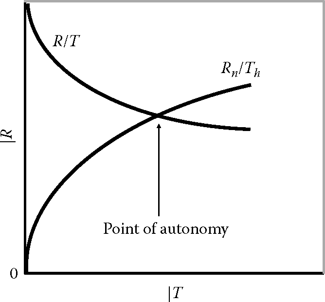
We have shown in previous work that the functions underlying the dynamic of T, R, Th, and Rn are production functions called the “Cobb–Douglas functions”, as follows48,49:
where Rn stands for “nonessential resources” and Th for “knowledge” or “technology.”
We also have
where T is “work” and R is “essential resources.”
We need to determine the value of alpha (α) as well as that of z or z′. My past research and database (see the chapter on People) lead us to the answer: when I assume z or z′ to equal 0 and set β0 as having a value of 1, the approximate value I find for alpha (α) is 0.3.
It is useful to hold one variable in both Equations 4.7 and 4.8 as a constant as otherwise the production function requires a three-dimensional approach that is challenging to plot. This treatment allows us to produce the graphs shown in Table 4.10.
The function [E′ = z′ − β0 Tα R(1 − α)] makes sense. As time goes on (as time is consumed during the project), the team members (Forces of Production) become more and more accustomed to their work, which ends up being routine. Less and less effort is required for the same set of tasks, but essential resources stabilize, much like people’s hunger levels reach a satiety point when fed, and yet they keep working: hence, the curve is descending. On the other hand, the function as set in Table 4.10 expresses the fact that management and team members (the Forces of Production), becoming more efficient, are able to stash larger portions of essential resources (thus turning them into nonessential resources), or else manage to save money to buy more nonessential resources (for the company/project) as the essential needs are answered faster and better than before.
| For the function: E′ = z′ – β0TαR(1−α) holding one variable constant (R = 1) | For the function: holding one variable constant (Th = 1) |
 | 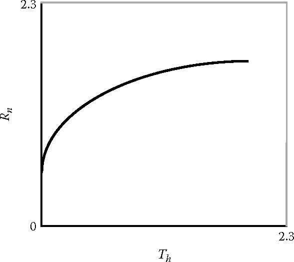 |
| 2.3 − T0.3 10.7 or (1 + k) − Tk−1 11−(k−1) | 0.3 + Rn0.3 10.7 or (k − 1) + Rnk−1 11−(k−1) |
Note again that by having a common variable among all of the key functions we have seen so far (k), we are justified to plot all the curves pertaining to a particular project on the same graph even though the abscissa and coordinate axes differ depending on the process element under review50 (see the multidimensional Table 4.20).

Note that all curves meet at the Point of Equilibrium: the U(DS), the project Blindness curve, the DS curve, and the two production curves R – T and Rn – Th. They all meet at [x = 1 and y = 1.3] within a closed dynamic system bound by the value of [1 + 1.3 = 2.3]. It is to the best advantage of the project manager to reach this Point of Equilibrium, because at that point, while POVs do exist, they are under maximum control by the team members (through R – T and Rn – Th) and in particular by management (DS curve).
At any point outside this Point of Equilibrium (POE),51 the following takes place:
- The project manager’s position may be temporarily improved but only to the detriment of the utility drawback (so that the utility drawback worsens)—in the end, the project is worse off.
- The project manager’s position may be temporarily improved but only to the detriment of the Forces of Production (FP), which then retaliate (becoming FPnc; e.g., by way of a strike or sabotage) so that in the end everyone is worse off.
There is no improving the position outside the Point of Equilibrium without alienating the project’s nature or the project workforce, or somehow a mixture of both. Put differently, the Point of Equilibrium is where there is the minimal number of POVs that ought to be managed. As project managers get closer and closer to the Point of Equilibrium POE (say at 99% or 0.99) the POVs approach zero. This observation is handy because POVs can hardly be measured directly: one of their core features is that they are often hidden truths, as we have previously discussed. While we do all we can, as feasibility analysts, to uncover them, we cannot be sure that we have uncovered them all. However, the way around this unchartered factor is to measure the Point of Equilibrium. It is perfectly feasible to establish measures for this point, and we are fortunate enough that all curves pass through this point, so that its measurement can rely on a number of angles of analysis. Recall that our initial objective was precisely to shed light on the project from different angles, to leave no shadows (hidden truths) around it. Each curve is a spotlight that illuminates the object—the Point of Equilibrium—so that no POVs can be left unknown. Examples of measures that can be taken include
- For the project Blindness curve: management style, realistic assessments of risks, and POVs.
- For the U(DS): consistency and stability of the project plan as it is conceived and implemented or, put differently, number/nature/salience of the changes, size and relevance of the infrastructures, and so on.
- For the DS curve: sick days, strikes, sabotage, wastes, delays, training, and so on.
As can be seen, the feasibility analyst is not short of measures that can help him assess, ahead of time, whether a project is likely to be a success or not. Otherwise, the expert can set his own list depending on the particularities of the project that he/she is working on.
Let’s assume now that all the forces that work in favor of the project, that is, the different curves we have examined so far (the project Blindness curve, U(DS) curve, and DS curve), behave normally and let’s set the Point of Equilibrium (POE) as the center point of a normal distribution curve. Refer to Figure 4.21.

The trick here is to determine what level of variance from the Point of Equilibrium (POE) is acceptable in order for the feasibility analyst to give the go-ahead for a project. Thus, the feasibility analyst has three main concerns:
- Determining the value and particularities of the POE.
- Determining the actual kurtosis and skewness52 of the normal distribution curve.
- Determining the acceptable levels of variance, with each sigma σ representing a different managerial decision (go—within one σ if we establish that the variance is to be minimized), rectify (between one and two σ’s), or no go (two or more σ’s).
The nice thing about this overall analysis is that it provides a mathematical framework upon which a feasibility decision can be based by relying not merely on technical, marketing, or financial evaluations alone, but most critically on POVs.
4.7.3 Final point of delivery
A project does not end because the desired output—say, a brand new building—is being delivered to its rightful owner. Measurements must be made that allow project managers to determine whether the triple constraints were respected, and to set formal knowledge that can help in future similar projects. Because we have defined projects as producing outputs—including deliverables, some form of a book of knowledge (BOK), and impacts—a project is not complete until such a BOK is finalized.
A helpful method is to identify the various magic moments of the project to see if measurements can be made at each of these points (especially in an evaluation of the POE) ahead of time, and as they materialize when the project is progressing. This is exemplified in Table 4.11.
| Magic moment | Date comments | Assessment during the project | |
|---|---|---|---|
| Costs associated with the slip-off | Nature of slip-off | ||
| Starting point | |||
| Point of autonomy | |||
| Point of no return | |||
| Final point of delivery | |||
In Table 4.11, the POVs, POE, and other points (stage gates, etc.) are put aside, with the emphasis being solely on the three process points past the starting point, which are regularly ignored or else treated lightly in feasibility studies. I contend that due consideration must be given to these points because they are intimately linked to the success of the project.
Note that the Point of Equilibrium (POE) is not a passage point; it exists within the framework defined by the utility drawback or triple constraints. This means that managers can stay on the equilibrium point at all times, providing they control the level of utility drawback, that is, providing they abide by the calendar of activities, do not exceed anticipated costs, and conform to the preset norms of quality. Hence, the Point of Equilibrium is really a dynamic Point of Equilibrium. We will see in Chapters 5 and 6 on People how dynamic it is: very much so, because when two people engage with it, games are played that make the point active (if not shaky) at all times.
4.7.4 G-rate and g-spread
We have talked about the variance around the Point of Equilibrium (POE). There is another way of looking at this variance: by expressing it along the different stages of the project. I refer to this variance as the “g-spread”, g standing for “growth.”53
Let us set the following scenario while doing a little bit of accounting: A given project is assumed to produce no sale and generate no income (even through investment activities). We set that profits will come in only once the final point of delivery is reached. In the meantime, there is no P&L statement54 worth the name. The project’s balance sheet contains, of course, the list of assets, liabilities, and equity. Applying these accounting terms in the field of project feasibility, we can say that the balance sheet includes the value of the deliverables (assets), the costs incurred or to be incurred (liabilities), and the value of the project (equity). Technically speaking and using an accountant’s approach, we want to have sufficient equity to cover the costs (i.e., [Value of project – Value of deliverables = Costs]). Any unplanned increases in costs will affect the project. We know that there is a relationship between each of the three constraints; we have discovered that when costs change, timing and norms of quality (established and controlled by the four Ps) constraints are affected.
Recall that the stages of a project over time are
| Vision | Planning | Mobilization | Deployment | Completion/evaluation |
Let’s decide that total sales from the project will generate US$5000 once completed, after 5 years. Each of the five stages of the project account for one-fifth of the planned total sales, or US$1000 per stage. We obtain the following result:
| Vision | Planning | Mobilization | Deployment | Completion/evaluation |
| US$1000 | US$1000 | US$1000 | US$1000 | US$1000 |
However, the time factor affects each stage in a particular way. The investment in inputs (resources, etc.) that is in the vision period is bearing fruit only along each of the subsequent stages. Somehow, we need to account for this; we add a growth factor, which we name “g”. This g (g-rate) is similar to an interest rate on a bank loan (sometimes called a “discount rate”) or a return on an investment. To facilitate our understanding of the present example, we set this growth factor, g, at a value of 10, 10 being the theoretical maximum value and 0 being the minimum value that the factor can theoretically reach. Rounding numbers, we obtain the future value of US$5000 by imputing US$820 per stage given a g of 1055,56:
| Vision | Planning | Mobilization | Deployment | Completion/evaluation |
| US$820 |g = 10 | US$820 | US$820 | US$820 | US$820 |g = 10 |
| |g = 10 | |g = 10 | |g = 10 |
Suppose that at the end of a given stage, managers have produced the deliverables (e.g., the foundation of a house) according to the planned schedule, costs, and norms of quality, we can state that the g-rate = 10; put differently, 100% of the production step has been completed. If the deliverables, costs, or timing, or a mixture of these elements have not met the expectations set at the end of the first stage, we would say that only 80%, for example, of that particular stage has been completed.
Yet, we want to keep our initial goal of total sales of the final project to US$5000. Therefore, the g-rate must be adjusted upward beyond the failing stage, since we set that sales (the US$820/step initially established) cannot be changed, and so that we have
| Vision | Planning | Mobilization | Deployment | Completion/evaluation |
US$820 * 80% = US$660 | g = 10 | US$820 |g = 10 To be adjusted | US$820 |g = 10 To be adjusted | US$820 |g = 10 To be adjusted | US$820 |g = 10 To be adjusted |
A simple calculation would show that the g-rate would have to be adjusted upward for the last four stages as follows:
| Vision | Planning | Mobilization | Deployment | Completion/evaluation |
US$820 * 80% = US$660 | g1 = 10 | US$820 |g2 = 12.5% | US$820 |g3 = 12.5% | US$820 |g4 = 12.5% | US$820 |g5 = 12.5% |
The reader can see that there is a difference between the maximum set of 10% and the g-rate necessitated by the production problems incurred during the first stage. This gap (called the “g-spread”) consists of 2.5 points (2.5%). A negative gap [real g – ideal g] indicates that there is something to be worried about. The team must work more intensely in the last four stages to catch up for the shortcomings encountered in stage 1. Thus, the gap becomes an indicator of shortcomings and a measure of POVs: the project has incurred delays, exceeded expected costs, and/or faced quality challenges that go beyond existing resources allocated to the project. The more difficulties that accumulate over time, the more the g-rate increases in value, because the remaining stages of the project must obligatorily compensate for past mistakes.
A negative g (a pessimistic scenario being realized) indicates that the project has fallen behind schedule, exceeded costs, or suffered from quality mishaps, or an amalgam of two or three of these problems. A moderate positive g (an optimistic scenario being realized), conversely, points to the fact that the project is progressing properly. The shape of the curve of evolution of the g-spread can be set as per the example in Figure 4.22.

A manager could want to fix the setbacks incurred in stage 1 (vision) only during stage 2 (planning), forcing g2 to increase to a whopping value of 24%, for a difference of [24 – 10 =] 14 points above the base g-rate. Accomplishing such a deed would probably entail that materials of lesser quality were used, payments of suppliers delayed, and so forth.
An overly positive g-spread is also a bad sign: the manager likely condones real problems, or else, tricks the delivery date (e.g., to receive a performance premium), reduces costs unduly (e.g., by cutting quality or fringe benefits granted to workers), and/or circumvents norms of quality (e.g., by ignoring certain standards).57
In summary, the g-spread is a temporal (longitudinal) representation of the variance σ around the project’s dynamic Point of Equilibrium, POE.58 The g-spread can serve as a representation of POVs. When it falls outside a certain upper or lower limit, this means that the project is vulnerable. Too much stress is imposed upon it. The g-spread highlights how critical the POVs are: the closer the project is to its deadline, the higher the value of g must be if there have been recent mishaps or cumulative problems. I assume that the total vulnerability is the sum of each g-spread along each of the five stages, so that
The third law of project feasibility is found to be the following:
4.7.4.1 The third law of project feasibility: The law of points of vulnerability
The higher the total vulnerability is (the sums of all g-spreads along each stage of the transformation phase) and the weaker the remedial actions are, the less the project is feasible.
The feasibility analyst is thus equipped with a punctual view of POVs—by looking at the project’s dynamic Point of Equilibrium (POE)—and with a longitudinal view of it.
4.8 Not-so-magic moments
We have identified key process points that are sometimes ignored when performing a feasibility analysis. Stage gates, benchmarks, and milestones have a positive connotation; even the points of autonomy, of no return, and the final point of delivery should indicate that the project has been proceeding along. There are, however, points that have negative connotations attached to them, I see them as the “little brothers” of POVs. They require some efforts at troubleshooting, a typical activity for both feasibility experts and project managers.
4.8.1 Triggers, red flags, concerns, bottlenecks, hurdles
Triggers serve as a spark plug for a causal flow that has negative consequences.
Red flags are warnings that something may be about to go wrong. Questions such as the following may be posed by a feasibility analyst:
- Were there any difficulties in meeting deadlines for presenting the proposed project?
- Are interruptions likely to be debilitating?
- Will staff accomplish what they are supposed to do every day?
- Will staff remain productive from start to finish?
- Are the project’s priorities likely to be respected?
These questions can be put in perspective when interviewing the project promoter who is seeking funding. His lack of preparedness or his overly ambitious plans are, certainly, red flags.
As I have established in the case of the Québec Multifunctional Amphitheatre (QMA), a list of preoccupations/concerns was made (see Table I.8). These may not be POVs just yet, but they may well develop into a vulnerability given that external risks affect the project in a certain way and with sufficient energy.
Bottlenecks occur during production. However, the feasibility analyst should review the forecasted production flows to verify whether bottlenecks are likely to develop. Surprisingly, bottlenecks are often due to human factors. Those experienced in driving in intense traffic are often witnesses to the fact that there are no obvious justifications for a particular traffic jam or sudden ambling. This phenomenon has been analyzed time and again, to the point that some cities have gotten rid of some sets of lights at specific intersections because city planners realized that the flow of traffic was more efficient when people were left to deal with each other rather than when being regulated.
Hurdles are temporary obstacles that may be anticipated. If so, they should not occur during production; of course, steps should have been taken to weed them out or to negotiate around them.59 As anticipatory events, they can be included in a feasibility analysis—they are an example of POVs.
4.9 Conclusion to Chapter 4
This chapter was dedicated to the second P of project management: Processes. We have seen four different levels of causation, something that no other books, I believe and to the best of my knowledge, have done in the past. We proposed a language to quickly explain project events and to help visualize the g-spread. Overall, Processes cannot be treated lightly: in reality, a feasibility study is, by itself, a project, so that it is naturally a reflexive effort. A feasibility study that is a well-processed project is likely to reach conclusions that are far more reliable than one that is vague, inconsistent, and that does not respect the rules inherent to process analysis, with its flow of inputs, transformations, and outputs.
4.10 What we have learned about POVs: Chapter 4
POVs…
- Become obvious when the direct linear process starts going astray.
- Can be awoken by uncontrollable factors.
- Can be detected when the project starts to be both ineffective and inefficient.
- Are brought under control when straight direct and diagonal processes work in tandem to achieve a result that is close enough to the intended output.
- That are hidden in a variety of entry points, end points, or nondirect flows will likely remain undetected until after they cause damage to the project.
- Always affect one or more of the three constraints: time, costs, and/or norms of quality.
- Cause havoc in the transformation phase of the project when the most critical linkage level is reached.
- Have four levels of criticality (low, moderate, serious, critical) depending on the nature of the causal bond in the process.
- Can be highlighted by the causal links appearing in the process (especially in a critical path assessment).
- Are more dangerous on the critical path than on paths where mediating options exist.
- Weaken any process system.
- Can be awoken by the catalyst effect of a moderating variable.
- Are sensitive to the types of process bonds (D, T, I, C).
- Grow like mushrooms (in dark areas).
- Can be anticipated to a certain degree.
- Can be identified through our modeling technique.
- Are to be considered by a manager along with: controlling risks, eliminating errors, managing the Unfits (uncontrolled Forces of Production, FPnc), harmonizing the four Ps, and relying on proper infrastructure.
- Have two faces: one with respect to the error term ε (linked to efficiency), and one with respect to the final outputs (linked to efficacy).
- Are temporal: they have to be measured in regard to inputs, outputs, and to the error term ε.
- Are empowered by the lack of forecasting of outputs.
- Are linked to the Blindness curve.
- Are linked to utility (a zero difference between beginning and end POVs suggests a high utility).
- Are not classified as magic moments.
- Can be somewhat reduced by having some excesses (Rn).
- Are at the highest level when far away from the POE.
- Can hardly be measured directly because they are often cloaked.
- Can be uncovered by analyzing the POE.
- Can be somewhat represented by the g-spread.
- Can be viewed punctually and longitudinally.
4.11 Key managerial considerations: Chapter 4
- Reduce all process flows to causal relationships.
- Seek equilibrium.
- Measure variance punctually and longitudinally.
- Use modeling and modeling language to extirpate hidden POVs.
- Be absorbed by three fundamental preoccupations, that is, managing and minimizing: risks, POVs, and ε, the error term.
4.12 Case study Chapter 4: Sea Crest Fisheries
4.12.1 Introduction
Sea Crest Fisheries (SCF) is based just off of Evangeline Trail, in the French-speaking sector of Northwest Nova Scotia, Canada, along the shores of the Bay of Fundy where there is an abundance of herrings, scallops, and lobsters. The company, founded by the father of the present president Brian Saulnier, was traditionally oriented toward herring fishing, with a large part of the business going to Japan—the Japanese are fond of herring roe. Brian has scintillating brown eyes and an abundance of energy, which he expands from 5 o’clock in the morning to late in the afternoon, supervising the plant, dealing with his suppliers, and entertaining his customers.
In the 1990–2000s, a growing business in the area was that of the farming of minks—mink fur was a much-coveted product among European and Russian customers in particular. On the other hand, the fish business in Europe witnessed a decline in sales and reduced profits due to lower market prices. In 1998, Sea Crest Fisheries was bought by four partners who saw an opportunity to control the supply of mink food for their local farms. As a result, Sea Crest’s vocation changed and included the manufacturing of mink food, produced with four basic key ingredients: fish, poultry, pork, and grain. The actual transformation process is very simple: it consists of mixing the four core ingredients (plus, in particular, some supplement mixes) with the right ratio to provide maximum feeding to the minks, thousands of them disseminated in a large number of farms located within the vicinity. Production losses are near zero.
The mink food business was not new to the owners of the company. They were clients who had been buying raw materials from it for years, and who made their own mink food on their local farms. However, at the start of 2000, the mink fur business grew exponentially, leaving little room for the farm production of mink food. It became easier and more sensible to buy prepared mink food from an external source. From this, the project of transforming Sea Crest Fisheries into a mink food–producing facility developed. The opportunity came from two opposing trends in the market: a reduction in the fish business and a surge in the demand for mink fur. By having numerous local farmers who were all buying from one source, the purchasing power of this group strengthened, thus leading to lower food costs for mink farmers. Furthermore, there was some form of synergy between mink food and herring: minks eagerly feast on herring.
4.12.2 The project
In 2003, a vision emerged whereby Sea Crest Fisheries would be mostly dedicated to mink food production. Brian Saulnier, president of the company, mentions
The project came out of a vision to see equipment and building assembled in a functional manner in order to produce mink food for which market demand and sales had previously been anticipated. I knew it had to be framed within a budget constraint and a specific timeline.
This became the goal set in 2005 for Sea Crest Fisheries (SCF): to build a plant devoted to producing mink food.60 The time line to accomplish this was within 12 months, at a cost of C$2MM (in the end, the project cost an additional C$5000), with norms of quality adapted to fit the requirements of the Canadian Food Inspection Agency (CFIA). Government regulations were, in fact, minimal because the industry was relatively new; however, Sea Crest preferred to be in a position where it could be prepared for anticipated regulations. The time line was somewhat critical because SCF wanted to start the operations in June 2006 so that it would have enough time to prepare and adapt to the peak production season, which occurs in August. However, delays in the installation of the electrical panels pushed the launch production date to the limit of early August. In a sense, this was the most pessimistic scenario happening: excess demand compared with actual production capacity. The original plan had been set in a realistic scenario of preparedness for June 2006, with no real optimistic scenario pushing production ahead of the scheduled launch date.
An informal list of stakeholders was prepared and concentrated on the owners, the clients, and the suppliers. The suppliers represented a risk by themselves because there was no certainty they could supply all the raw material needed for the two formulations that ended up being chosen by the SCF team. SCF had a backup plan though: in case of shortages, inputs such as poultry, herring (which came plentifully and was SCF’s original main business) would be used. The project manager and final decision-maker on the evaluation of the project was Brian Saulnier and it is he, also, who prepared an informal project charter, not the actual sponsors of the project. He was given carte blanche in about every aspect of the project. Hence, the organization was neither traditional nor a matrix, but rather purely project oriented. Of the three aspects of POW (Product, Organization, and Work) Breakdown Structure, it is the WBS that caused the most difficulty up to the present day. According to Brian:
This is an area where we learned we should have done things differently. Recall we had a business that was mostly based on temporary work and limited skills; the work load evolved with the fishing season. However, with the mink-producing plant, we moved to full time, year-long jobs. Yet, employees never had a job description. Hence, they acquired rights and privileges that at times were counterproductive and that we could not, as managers, change for lack of proper procedures. We are still experiencing difficulties in this area nowadays, albeit they are being addressed.
An informal survey was done to assess potential customers’ needs. The process was rather informal given the nature of the close-knit community. How many minks would be fed and how many different formulations would be needed? As it turned out, each mink grower had developed his own formulation; variations between the different formulations were wide ranging, for example, from 15% to 70% in herring content. In the end, however, two formulations satisfied 100% of the customers, with 80% having chosen one formulation, and the balance, 20%, having chosen another one.
Cost analyses and break-even points were established based on expected prices and volumes. However, new infrastructure and new equipment were needed, with the latter eventually bought from a company in Finland. In 2003–2004, Sea Crest built a freezer out of which items such as chicken and herring were shipped to local farmers. In 2004–2005, the floor layout for the upcoming mink-producing plant was prepared, but the owners soon realized its surface had been understated as the mink fur business grew faster and faster; at some point, the growth rate was about twofold every 6 months. Once landed, the Finnish equipment was installed by local crew and a local company was hired to set up the electrical system and control boards. In 2006, some 40% of the 35 employees marshaled in the new business; the first test, ran in August, took 12 hours to produce 11,000 lbs. As of 2015, some 95% of the 50 employees are bustling producing a batch every 7 min, with a maximum production of 800,000 lbs/day during the busiest month of August. This translates into an average of 13 trucks delivering food to local farmers every day. Between 2007 and 2015, annual production grew by 325%.
Fortunately, not all clients converged toward the newly built plants at first, although demand was certainly very high during the month of August 2006; some farmers kept on producing their own mink food for a while until they realized it was more economically sound to outsource to Sea Crest. Also playing in Sea Crest’s favor was the limited level of regulation in the business of mink food production and the mink farming business (a situation that is changing fast due to river and land pollution the likes of which had been seen for decades in many parts of the country with pig farming).
In short, the main milestones and stages of the project were
- September 2005: Ordering the equipment from a Finnish company
- October 2005–February 2006: Building the production, refrigerator, storage, and warehouse areas
- February 2006–July 2006: Installing the electrical wiring and panels
- August 2006: First production batch
The project was innovative in three ways from SCF’s perspective: (1) the company had never produced mink food before and its business had mainly been in extracting herring roe from herring fish for shipments overseas; (2) new equipment had to be bought for which SCF had no experience and which needed to be complemented with an adapted design to fit its needs—in fact, the entire control room systems, the electrical panels, and the plumbing were done in house; and (3) the formulations had to be redesigned to meet the majority of the growers’ needs, with the help of a research facility attached to a local university.
Using the PMBOK terminology,61 the project can be seen as a series of groups of processes. The initiating group of processes encompasses the different stakeholders who had a vision for a new plant. Processes per se were focused on listening to future clients’ needs.
Persons and Power were easily chosen and established, as Brian Saulnier had all the latitude he needed. The planning group of processes (we are still using PMBOK terminology) included a financial plan that was presented to a government-sponsored bank.
A firm calendar was adopted as well as norms of quality (based on government standards). The executing group of processes saw Brian Saulnier ensuring that the plan was being respected and that the processes matched their preset flows (although there were no formal PERT or critical path methods used). Persons that participated in the execution stage included an external contractor for building the actual plant and another one for the electrical system (which proved to be the cause of the delay, starting in February 2006); internally, the mechanics formerly employed to handle machinery related to herring processing were diverted to supervising the new equipment implementation. The mechanic with the most expertise was chosen as an informal second-in-command. Much of the work was done informally using a “learn as we go” rationale.
The monitoring and controlling group of processes was minimal and, again, rather informal. No major modifications were necessary versus the initial plan, except for relocating the ladder that gives access to the control room. No log books were prepared to keep track of modifications, however. Brian and his second-in-command had heartfully intended that the project progressed as initially envisioned.
The closing group of processes experienced some challenges. As mentioned, the closing stage took place toward the end of July rather than at the beginning of June due to difficulties with the installation of the electrical system. A final report was needed by the bank. New employees had to be hired (seven in total) when production started and a new managerial job was devised, that of feed kitchen manager (two people, one each for the day and night shifts).
The sociocultural risk associated with the business stemmed from pressure groups that oppose the killing of animals in fur production. In the United States, a large fur plant had been set ablaze by frantic activists. Internally, two major current POVs come to mind. First, while the plant manager masters the plant’s processes and follows up on postproduction testing in its laboratory, many incoming raw materials present some form of contamination (e.g., chicken), which could spread internally. Second, the plant has become the largest and quasi-exclusive producer of mink food (there is another producer nearby—Nova Feeds, of a smaller size); the concern is that it has only one line of production, with few spare parts and backup Means of production (e.g., grinders, mixers) available, so that any major production glitch would virtually shut the plant down and threaten the survival of some of the local mink farms. It would be enough for a risk-factor-turned-POV (an outside activist hiding his intentions and getting hired to work on the production line) to target a vulnerability point (the entry point of raw material or the production line itself) and sabotage it to cause a business disaster.
Environmental concerns arose chiefly from noise levels: local inhabitants complained about trucks driving in and out of the plant at any time of the night. Strict transportation schedules and on and off loading rules were set to minimize noise levels.
One of the biggest baskets of risks and vulnerabilities was the divergence between the various external and internal stakeholders.62 The tight network of the community helped in solving the issues at hand and in ensuring an overall positive business climate.
No doubt, Brian Saulnier’s personality played an instrumental role in keeping all parties content. He is a laid back leader who trusts his staff and who dislikes confrontation, favoring instead mediation and compromise. His realistic and pragmatic views add to his skills and reinforce the respect his staff displays toward him. His management approach is not about status games, but about being reasonable, believing in people, and encouraging them to do their best. Face-to-face exchanges instead of e-mails are a preferred method of communication. Meetings are kept to a minimum; walking through the plant as it is being built is worth more than sending directives without knowing exactly what happens on the ground.
Business has been good for Sea Crest Fisheries. As stated by Brian Saulnier:
We are a small part of the country. Here, business is done with handshakes, not with lengthy, overly complex contracts. We have close bonds with the employees and our suppliers and everyone out there seeks to help one another. Management shows gratitude by way of flexibility, for example, with vacation allowance and bonus pay. If I have to summarize our project, it was all about loyalty.
China, however, has entered into the equation. It has long been a substantial buyer, but it now has become a provider of mink fur, with its own methods; add to this its control of its exchange rates on the international scene to facilitate its exports.
4.12.3 Quality audit
A quality audit was performed in 2015–2016 to verify whether improvements could be made to reduce the possibility of contamination. The plant was examined in two different conditions: the first one during idle hours, when no production was taking place and the second condition, discussed in the next section, took place during production.
A tour of the plant was done, observations made, pictures taken, and questions posed. Two categories of observations were listed in the final report: one relating to quality control, the other one relating to safety and security (i.e., relating to costs). A third look at the plant focused on time, that is, on efficiency, maximizing the various flows of personnel movements.
With respect to quality control and the risk of contamination, the following notes were prepared, which are completed with recommendations.
4.12.4 Inputs: Quality audit
Major product inputs include poultry, pork, grains, and fish; antibiotics and vitamins are also added. Poultry is the main source of contamination, especially in the summertime. Two options are readily available: to put all arrivals in quarantine until tests (salmonella and Escherichia coli) are done and the product is released, or else to incite the supplier to arrive on the deck with a certificate of conformity. The first option does not solve the problem of what to do with the rejected product (return it or destroy it). This may cause tensions with the supplier, just as the second option would do. Poultry coming in is currently tested in the plant’s laboratory, but it happens that the poultry has already entered the production line before the results are out. This practice is not recommended.

As mentioned, there are a number of options to deal with poultry contamination, which can reach elevated levels during the summer.
First, there could be a monitoring system at the shipper’s end; however, little control or enforcement can be exercised. Control upon arrival is standard, of course, but at times production rush requires to use poultry right away. At other times, a poultry truck may sit for quite some time outside, in the sun, because of holidays, weekends, or timing related to production.
An option to reduce contamination is to use dried poultry meat (supplied by Nestlé Purina); however, this entails changing the formulation (which is at the heart of the operation and which at last was agreed upon with the mink farmers). In addition, the dried ingredients tend to jam some pipes and screws in the facility, where the mink food is so-called wet food rather than dried (in kibbles).
Acid is put into the formula in an effort to lessen the potential for contamination, but its use is limited for obvious reasons.
Another option (currently partly used) is to freeze all chicken meats—however, to destroy bacteria effectively, the freezing has to be intense. This can be costly and may delay production at times.
Fortunately, to date, contamination has not proved to cause harm to the minks. However, stronger controls are required.
The other entry point that causes concern is the trap set to channel incoming fish shipments.
This trap is located along the side of the main production building. It has no cover; an errant or curious rodent attracted by the smell could climb it and fall down the pipe that ends in the hopper. This trap should have a cover when not in use.

The room where additives (antibiotics, vitamins, etc.) are kept is also of concern. The area is hardly sealed and the product sits on pallets, which sit on the floor.
Typically, such pallets should be shelved, with the bottom shelf roughly 2 feet above the floor (mice can jump about that high). In addition, there should be a space along all the walls of about 2 feet to deter rodents from traveling in dark alleys and to facilitate inspection. Sea Crest Fisheries should check whether the antibiotics require special storage conditions such as room temperature and humidity levels.

Entry materials—poultry, pork, and fish—should pass through a metal detector, which has not yet been installed. Pallets must also be inspected—a procedure must be set for such quality control concern. Old, damaged pallets may include wood splinters and nails that can get into the food or else that could allow mold to grow.
Hidden storage space: There is a space that is difficult to access where rodents and bird droppings have been noticed, with no signs of pest control.
Employee’s kitchen area: This room is filthy. Employees must learn to keep the place impeccably clean. There are many entry points for mice but one single mouse trap is located beneath the sink.
4.12.5 Transformation: Quality audit
During the transformation phase, a number of areas present a potential for contamination.
Hopper: There is a hopper beside the main processing units and mixers where access is obviously difficult. As a result, the hopper and the pipe do not appear to be perfectly clean; mold can likely develop, bacteria can easily grow given that the ambient temperature, and humidity levels are high.
Large hoppers: There is a room besides the main processing room that contains large hoppers, some of which do not appear to be completely clean.

Ring: There is a ring that is not made of stainless steel and that is painted—this can cause metal/paint particles to enter the food. The paint should be shaved off the rings.
Sitting products: Some pallets of products sit before the entry leading to the freezer where they are being thawed to room temperature. As the product defrosts, it tends to spill on the floor. A space of about 2 feet should separate the pallets from the walls and the pallets should be encased by rails so that circulating individuals and forklifts don’t tend to touch them. The pallets should preferably be put above the floor so that contaminants carried on the boots of employees do not readily access the food. The time and day at which the pallets are left to defrost should be indicated on the pallets and recorded in a registry to guarantee traceability.

Pipe: One of the pipes has been hammered several times in order to let the content slide through gravitationally.
This suggests that the formulation is too thick and that some of it may actually be stuck inside, potentially allowing bacteria growth.
Vitamin input: The information on the formulation is written manually on a piece of paper. There should be a software program that manages all aspects of formulation in order to secure traceability.

Control room: The control room is filthy and it was noticed that the operator smokes in it (because a concealed ashtray was found after smelling the cigarette smoke), despite having been advised not to do so for two years. There is a dead spot where he cannot see part of the production (especially on top of the stairs near the mixers)—mirrors should be installed to cover dead spots. Even though there are cameras, this may skip the attention of the controller; should the person emptying his bucket of vitamin content inside the mixer be in trouble, there are no alarm buttons on the upper floor.
Cleaning during production: A couple of employees kept the floors clean during production. Overall, the plant is tidy.

4.12.6 Outputs: Quality audit
Output products are tested in two ways: (1) at the Sea Crest laboratory and at the independent Nova West laboratory, located in a remote location, where measurements include ash, fat, moisture, protein, and as E. coli counts. This double-check attests to the fact that the data are accurate. Sample batches are well identified.
4.12.7 Relationship between the appreciation of management and quality
SCF performed a quality audit in March 2016 based on an approved questionnaire aimed at measuring the relationship between the appreciation of management and quality. This effort was deemed useful in order to statistically measure whether the general appreciation of management (in essence, the project and operation leader—Mr. Brian Saulnier) meant higher concerns for quality work and control on the part of employees. Based on preliminary exploratory results,63 a simple statistic was computed and the data shown in Table Case 4.A were obtained.
“Dependence” relates to the participant’s (employee’s) need for his job, “Trust” relates to how much the participant feels he that can count on the top manager, “Fairness” relates to his perception of being treated fairly, “Collaboration” refers to the collaboration that exists between the participant and top management, and “Quality” expresses the effort made by the employee toward ensuring quality standards are met or exceeded. Levels of Dependence, Trust, Fairness, and Collaboration are normal and are typical of so-called relational interactions. Both higher and lower numbers would indicate potential conflicts. The level for the construction of Quality is positively high, which speaks strongly in favor of SCF.
| Dependence | Trust | Fairness | Collab. | Quality | |
| Mean | 75 | 81 | 77 | 71 | 91 |
| Std. Error | 19 | 12 | 18 | 18 | 13 |
| Minimum | 14 | 54 | 36 | 31 | 57 |
An initial multiple linear regression analysis shows that the so-called psychological core ([Trust + Fairness + Collaboration]/3) is significantly related to quality (at p > 0.05), with an adjusted R2 of 0.425.64
Hence, it can be said that the plant is well managed and that this is an important factor in the achievement of quality standards, within the limits of this exploratory research. Indeed, an initial factorial analysis (25 iterations, varimax rotation) shows that when Conflicts are near zero, quality improves while when Conflicts approach 100%, quality deteriorates (refer to Table Case 4.B).
| Construct | Group 1 | Group 2 |
| Fairness | 1 | 0 |
| Conflicts | 0 | 1 |
| Trust | 1 | 0 |
| Collaboration | 1 | 0 |
| Quality | 1 | 0 |
Let’s now move to a simple cost-based audit, looking for areas where costs would be incurred in case of an accident or where they are currently incurred because of certain managerial practices.
4.12.8 Inputs/transformation/ouputs: Simple cost audit
Untidiness: In many areas, including in the electronic board control area, the maintenance area, and receiving area, various items are left sitting idle, such as buckets, coffee cups, hammers, rollers, and so forth. This is cumbersome and distracting and may actually cause an accident. This requires employee training.
Loose hoses were noticed, especially in the final output hopper area where the trucks wait. An employee could potentially trip and either fall into the hopper, with no chance of escaping alive, or fall two storeys down onto the concrete floor.
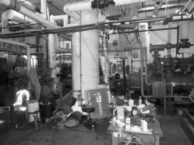
Language: Language is not uniform. Some employees speak English only while the Francophones are all bilingual. In case of emergencies, it is not certain whether Anglophones would understand the instructions or not, if expressed in French. Employee training is warranted.

Forklifts: Another safety concern is with respect to the loading areas for the forklift that are near to the robotic equipment. A stopper should be installed on the floor to prevent a forklift from hitting the conveyor.
The forklifts do not emit a loud enough noise when backing up, this may lead to an accident.
Emergency: There are a number of emergency devices that are well positioned, especially near the acid bin.

Documentation: The material safety data sheets (MSDS) all seem to be readily available in case of acid spillage. The pallets are identified with a ticket that is sent for entry into the computer system once the pallet is being moved to be unloaded. The formulations are entered by hand; as discussed, this should be done through a software program.
Follow-up forms are readily available and information is entered into a computer tracking system. However, the forms should include the time of the operations for better traceability. Units of measurement must be neatly identified on all production sheets (e.g., lbs).

4.12.9 Conclusion
The project of implementing a brand new plan for producing mink food has gone remarkably well, despite not having respected all of the project guidelines provided by the PMBOK. This is due in large part to the kind of close, friendly, and mutually trusting relationships that existed and still exist among all internal and external stakeholders. The operation is well run. The point of autonomy (the point at which the operation could run by itself without additional training or efforts) was achieved in October 2006 as far as machinery handling goes, and somewhere around June 2007 as far as formulations are concerned, for the mere fact that some formulations could not be tested before due to the seasonal nature of the mink farming business.
4.12.10 Appendix A of Case 4: Floor plan and construction65


4.12.11 Appendix B of Case 4: Production


4.12.12 Questions related to Case 4—SCF
- Describe the opportunity that arose and that led to the establishment of the mink food business.
- Draw the production process using the methodology taught in this book.
- Write the production process as explained in this book.
- Describe the five stages of the mink project life cycle, including the vision stage.
- List the People involved, including the regulators and the bad apples.
- Discuss the triple constraints, including the calendar.
- Refer back to the teachings of the PMBOK and identify the core elements such as the project charter and the management process groups.
- Discuss the POW.
- What is your take on the needs analysis?
- Identify and discuss magic moments.
- In what way was the project innovative?
- Discuss the four Ps.
- List the POVs that you can identify in the initial project and discuss their characteristics, presence, and importance.
- Position the POVs along the entire production chain.
- Identify and discuss the risks.
- Discuss the norms of quality and determine what steps can be taken to improve quality.
- Discuss the relationship between quality and management appreciation.
- Discuss the role of infrastructure, risk, and robust management.
Endnotes
- The PMBOK refers to five groups of processes (integrating, planning, executing, surveillance and control, and closing); however, as I shall discuss further along in this book, these are not processes per se, at least not the way they are explained. This being said, PMBOK 5 also seems to make some additions from a modeling point of view on p. 59: it introduces the process of “overall project control” which does not appear in its main matrix. This highlights the importance of using simplified models and of carefully integrating constructs or processes that are a vital part of the set project. Similarly, on p. 61, I could argue that knowledge area “9. Project HR Management” is in fact a subcategory of knowledge area “13. Project Stakeholder Management” since among the project stakeholders are those who benefit from a HR Management plan. Note that the word “direct” in Section 4.2 of p. 61 refers to a controlling activity (a Power activity: to direct) and thus does not really belong in the so-called executing process group. A better word given the context and the four Ps structure that I propose would be “implement.” I feel that “Initiating process group” and “Planning process group” belong to Planning, “Executing process group” and “Closing process group” belong to Process, and “Monitoring and controlling process group” belongs to Power. From my modeling point of view, it would be more attuned to production logic to have a functional activity group separated under: Plans, Process, People, and Power.
- For example, TSO, p. 21.
- Ryan and Bernard (1994, p. 782).
- Olivier and Payette (2010, p. 18).
- The goal of this book, however, is not to delve into PERT, the CPM, activity-on-node (AON) or activity-on-arrow (AOA), and precedence diagram methods. Plenty of books are available on the subject. See, for example, Devaux (2015). The French version of PMBOK 5e edition makes an error on p. 156 when defining finish-to-start and start-to-finish, using exactly the same definition for two different concepts.
- I developed this method and it has been the subject of various articles and of three books, one published by Springer Psychology.
- Note: The codes are in parentheses because that’s the way they appear in a modeling diagram, where they are positioned on the arrow linking two constructs.
- For example, see Goldfried and Davison (1994, p. 26).
- Creswell (1994, p. 85) states: “Position the dependent variable on the right in the diagram and the independent variables on the left.”
- Names and location have been altered to ensure confidentiality.
- The logic behind the group of processes promoted by PMBOK 5 is not necessarily truly functional in real life. PMBOK attempts to separate the five groups of processes it has identified from the life cycle stages of a project, when in fact they make a whole lot more sense, from my modeling point of view, when integrated into this life cycle. Additionally, the name “group of processes” is troublesome because the model is somewhat erroneous: there are inputs for sure, but there are no actions that follow—only tools and techniques are listed, which then presumably lead to outputs. However, tools and techniques are not a transformation action that move inputs into a category called outputs; from a modeling point of view, they are a Means of Production and hence, an input. Truly, the groups of processes are simply core functional activities. The complexity of the links between the groups of processes, their inputs, actions, and so-called outputs point to the fact that they must instead be considered as managerial activities that certainly have some logical flow, but that include a vast array of iterations and connections. All process diagrams have inputs, an action phase called transformation, and outputs.
- In the strictest of terms, POVs have affected first costs (risks affect time and errors affect norms of quality).
- I changed the names and locations to preserve anonymity.
- Each model and submodel must be kept to a minimal level of complexity. Many studies suggest that most people rely on a maximum of three, and at times four pieces of critical information to decide, act, and live.
- In some settings such as museums, humidity is a truly set parameter rather than simply a factor of influence.
- PMBOK 5 (2013, p. 157).
- In some network systems, Z would be called a “node”.
- When it comes to neuroscience (on which I will draw substantially in Chapter 7), one refers to structural connectivity as a “set of physical or structural (anatomical) connections linking neural elements” and to functional connectivity as “patterns based on time series data from neural recordings” (Sporns, 2011, pp. 36–37) where interdependence between neurons is recognized. An element of time (in milliseconds) is included in the definition because of the connectivity component of the term.
- Jarvis et al. (2003).
- Bollen and Lennox (1991, p. 308).
- See Diamantopoulos et al. (2008).
- Collier and Bienstock (2009, p. 284) mention that formative variables in statistics are theoretically uncorrelated (or sometimes negatively correlated, a statement I disagree with in the context of my methodology).
- Recall we use an error term with a negative sign for reasons we will see further along in this book.
- One must be careful; the terminology here is different than the one found in statistics for continuous data. An example of a continuous data in statistics is weather: it can be of 12 degrees, 12.5, 12.3, or 15, and so forth to an infinity of possibilities. In my example, continuous means a scale composed of more than two measurement units; in other words, any scale that is not binary (yes/no).
- Do not use present = 2 and absent = 1, that is, use only 1 and 0 to express the binary nature of a scale. Doing differently could cause difficulties when running statistical analyses or when creating mathematical formulae.
- The term “structural” is not related to structural equation modeling (SEM).
- One of the reasons why the analyst needs at least two process elements to form the main process element stems from the fact that he may want to define a process element by what it is and what it is not (black and white). Therefore, a main process element is necessarily formed by at least two subprocess elements. In the context of POVs, this is especially important. White cells in the body, for example, attack invaders by recognizing which bacteria are part of self (and our body contains billions of bacteria) and which are not. The immune system (which ensures there are no POVs left to the open) is dependent upon this differentiation between “self” and “not self.”
- See Diamantopoulos and Winklhofer (2001); Diamantopoulos and Siguaw (2006).
- Large projects normally, however, produce deliverables, accumulate some formal knowledge, and generate impacts.
- A useful method to identify the functional variables defining a process element or any object of investigation (e.g., a construct) is to churn out a list of questions that the analyst would want to pose to five different experts on said theme. This forces the analyst to envision what the said theme could do; by actually collecting answers from experts, functional variables have an even better chance of being fully identified.
- The Québec’s Nordiques, a fierce rival to the legendary Montréal’s Canadiens.
- Delahaye (2015, p. 78).
- Guardian (2013).
- Real name and location.
- If we equate infrastructures to 1 (or 100%), we obtain the formula for the Utility of the Dominant strategy U(DS).
- I show a stylized version of the rectangular hyperbola, and only a portion of it: the one that is significant for my study.
- For example, the project manager would think of himself very highly and consider that there are no POVs in his project or else he chooses to be oblivious to them.
- We will see in the chapter on People why it is near −1 and not exactly −1.
- For example, it has run some trials with inexperienced or uncommitted staff knowing the output will not be to the level of quality that is ultimately demanded.
- This initial value was found out from a longitudinal study I did and which we examine in Chapters 5 and 6 on People.
- This function is hypothetical: it is an attempt to portray how behaviors relating to a Dominant strategy look like. It was developed through a series of transformations operated on my core functions.
- From this perspective, we could refer to the new machine as an MPnc, that is, a Means of Production that is not yet controlled/mastered.
- T is for “Travail” which means “work” in French.
- As an example, the WBS was set by using the computer-based project planning and scheduling (CBPPS) system software during the 1988 Olympic Games in Calgary.
- Note that FPnc being considered a structural process element of FP, means that there cannot be a project without FPnc; we have seen in the section on innovation why that is.
- De Fraja (2009, p. 51).
- Cats are wiser than dogs in this respect; they only eat what they actually need, and they are very fussy on their choice of food. In fact, cats, unlike dogs, need taurine in their diet, because they don’t produce it naturally. Thus, taurine is an essential resource, without which they die.
- I do not include an error term in order to facilitate my presentation.
- We have seen that R and Rn entertain a contrasting relationship. When an individual accumulates essential resources R, he cannot gather nonessential resources Rn at exactly the same time. For this reason, in the output functions, R and Rn are presented in a different order: where Rn comes first, and [E′ = z′ − β0 Tα R(1 − α)], where R comes second.
- Otherwise, the graph would have to be multidimensional. For simplification, I do not name the axes directly on the graph.
- This will become clearer in the chapter on People.
- I suspect they change according to the type and size of projects.
- The literature on project management is not short of valuable concepts with respect to quality concerns, such as the notion of schedule variance, cost variance, and schedule performance index.
- Profit and loss statement.
- There is no initial investment and measurements are taken at the end of each stage, not at the beginning of the stage.
- Read, for example: US$820 | g = 10 → US$820 given g = 10.
- Structures such as bridges that collapse because of preventable construction defects provide an example. Often, construction materials have been deliberately chosen for their price regardless of their low quality, or else normal construction procedures have been short cut.
- In typical project management literature, one speaks of upper and lower control limits (according to quality expectations) and specification limits (according to needs) in a control chart. An accepted heuristic is the rule of seven by which any set of seven or more points appearing consecutively in either the lower or upper range (on one side of the mean) is considered not to be a random occurrence, suggesting the process is actually out of control.
- See Harrison and Lock (2004).
- This paragraph is in line with the concept of a “project charter” used in the PMBOK 4 (2008). A Guide to the Project Management Body of Knowledge—Fourth Edition. USA: Project Management Institute.
- The Project Management Book of Knowledge (2013), 5th edition, proposes five groups of processes, which I subdivide into Plan, Processes, People, and Power (authority).
- Indeed, a project feasibility analyst must look for divergence of interests as an important source of points of vulnerability.
- I intend to perform analyses that are more complex in the near future.
- F = 21.666 and sig. = 0.000. Residuals are normal. Durbin–Watson is acceptable at 2.580.
- Pictures in Appendix A of this case have been graciously provided by Mr. Brian Saulnier, president, Sea Crest Fisheries.
- Many psychometric or marketing questionnaires are built in order to boost the Cronbach’s alpha, regardless of sound psychometric rules. See work by the authors on the subject in the bibliography.
- Interestingly enough, when I take the standard network formula for calculating communication channels, [n(n − 1)/2] and find the value of n to achieve the k constant of 1.3 (more precisely 1.32), I obtain n = 2.2, which is the upper limit of the Blindness curve. The average k for many groups I studied is actually often 1.32 or near this value. For fun, I found that 1.32 = 1 + 1/π, and had a drink afterward!