Chapter 4

Getting Started with Arithmetic

In This Chapter

Using R as a fancy calculator

Constructing and working with vectors

Vectorizing your calculations

Statistics isn’t called applied mathematics just for the fun of it. Every statistical analysis involves a lot of calculations, and calculation is what R is designed for — the work that it does best.

R goes far beyond employing the classic arithmetic operators. It also contains sets of operators and functions that work on complete vectors at the same time. If you’ve read Chapter 3, you’ve gotten a first glimpse into the power of vectorized functions. In this chapter, you discover the full power of vectorization, using it to speed up calculations and perform complex tasks with very little code.

We can’t possibly cover all of R’s mathematical functions in one chapter — or even in one book — so we encourage you to browse the Help files and other sources when you’re done with this chapter. You can find search tips and a list of interesting sources in Chapter 11.

Working with Numbers, Infinity, and Missing Values

In many low-level computer languages, numerical operators are limited to performing standard arithmetic operations and some convenient functions like sum() and sqrt(). For R, the story is a bit different. R has four different groups of mathematical operators and functions:

Basic arithmetic operators: These operators are used in just about every programming language. We discuss some of them in Chapter 2.

Mathematical functions: You can find these advanced functions on a technical calculator.

Vector operations: Vector operations are functions that make calculations on a complete vector, like sum(). Each result depends on more than one value of the vector.

Matrix operations: These functions are used for operations and calculations.

In the following sections, you get familiar with basic arithmetic operators, mathematical functions, and vector operations. We cover matrix operations in Chapter 7.

Doing basic arithmetic

R has a rather complete set of arithmetic operators, so you can use R as a fancy calculator, as you see in this section.

Using arithmetic operators

Table 4-1 lists some basic arithmetic operators. Most of them are very familiar to programmers (and anybody else who studied math in school).

Table 4-1 Basic Arithmetic Operators

Operator	Description	Example
x + y	y added to x	2 + 3 = 5
x – y	y subtracted from x	8 – 2 = 6
x * y	x multiplied by y	3 * 2 = 6
x / y	x divided by y	10 / 5 = 2
x ^ y (or x ** y)	x raised to the power y	2 ^ 5 = 32
x %% y	remainder of x divided by y (x mod y)	7 %% 3 = 1
x %/% y	x divided by y but rounded down (integer divide)	7 %/% 3 = 2

All these operators are vectorized. Chapter 3 shows the use of a vectorized function with the paste() function, and the process works exactly the same way with operators. By using vectorized operators, you can carry out complex calculations with minimal code.

To see how this works, consider these two vectors, which we first discuss in the All-Star Grannies example in Chapter 3. One vector represents the number of baskets Granny made during the six games of the basketball season, and the other one represents the number of baskets her friend Geraldine made:

> baskets.of.Granny <- c(12,4,4,6,9,3)

> baskets.of.Geraldine <- c(5,3,2,2,12,9)

Suppose that Granny and Geraldine decide to raise money for the Make-A-Wish Foundation and asked people to make a donation for every basket they made. Granny requested $120 per basket, and Geraldine asked for $145 per basket. How do you calculate the total donations that they collected for each game?

R makes the calculation easy. First, calculate how much each lady earned per game, as follows:

> Granny.money <- baskets.of.Granny * 120

> Geraldine.money <- baskets.of.Geraldine * 145

In this example, every value in the vector is multiplied by the amount of money. Check for yourself by taking a look at the values in Granny.money and Geraldine.money.

To get the total money these ladies earned in each game, you simply do this:

> Granny.money + Geraldine.money

[1] 2165  915  770 1010 2820 1665

You also could do this in one line, as follows:

> baskets.of.Granny * 120 + baskets.of.Geraldine * 145

[1] 2165  915  770 1010 2820 1665

Controlling the order of the operations

In the previous example, you used both a multiplication and an addition operator. As you see from the result, R correctly multiplies all numbers before adding them together. For all arithmetic operators, the classic rules for the order of operations apply. Calculations are carried out in the following order:

1. Exponentiation

2. Multiplication and division in the order in which the operators are presented

3. Addition and subtraction in the order in which the operators are presented

The mod operator (%%) and the integer division operator (%/%) have the same priority as the normal division operator (/) in calculations.

You can change the order of the operations by using parentheses, like this:

> 4 + 2 * 3

[1] 10

> (4 + 2)* 3

[1] 18

Everything that’s put between parentheses is carried out first.

You also can use basic operators on complex numbers. The complex() function, for example, allows you to construct a whole set of complex numbers based on a vector with real parts and a vector with imaginary parts. For more information, see the Help page for ?complex.

Using mathematical functions

In R, of course, you want to use more than just basic operators. R comes with a whole set of mathematical functions that unleash fantastic numerical beasts. Table 4-2 lists the ones that we think you’ll use most often, but feel free to go on a voyage of discovery for others.

R naturally contains a whole set of functions that you’d find on a technical calculator as well. All these functions are vectorized, so you can use them on complete vectors.

Table 4-2 Useful Mathematical Functions in R

Function	What It Does
abs(x)	Takes the absolute value of x
log(x,base=y)	Takes the logarithm of x with base y; if base is not specified, returns the natural logarithm
exp(x)	Returns the exponential of x
sqrt(x)	Returns the square root of x
factorial(x)	Returns the factorial of x (x!)
choose(x,y)	Returns the number of possible combinations when drawing y elements at a time from x possibilities

The possibilities of R go far beyond this small list of functions, however. We cover some of the special cases in the following sections.

Calculating logarithms and exponentials

In R, you can take the logarithm of the numbers from 1 to 3 like this:

> log(1:3)

[1] 0.0000000 0.6931472 1.0986123

Whenever you use one of these functions, R calculates the natural logarithm if you don’t specify any base.

You calculate the logarithm of these numbers with base 6 like this:

> log(1:3,base=6)

[1] 0.0000000 0.3868528 0.6131472

For the logarithms with bases 2 and 10, you can use the convenience functions log2() and log10().

You carry out the inverse operation of log() by using exp(). This last function raises e to the power mentioned between brackets, like this:

> x <- log(1:3)

> exp(x)

Again, you can add a vector as an argument, because the exp() function is also vectorized. In fact, in the preceding code, you constructed the vector within the call to exp(). This code is yet another example of nesting functions in R.

Putting the science in scientific notation

The outcome of the last example may look a bit weird if you aren’t familiar with the scientific notation of numbers. Scientific notation allows you to represent a very large or very small number in a convenient way. The number is presented as a decimal and an exponent, separated by e. You get the number by multiplying the decimal by 10 to the power of the exponent. The number 13,300, for example, also can be written as 1.33 × 10^4, which is 1.33e4 in R:

> 1.33e4

[1] 13300

Likewise, 0.0412 can be written as 4.12 × 10^–2 , which is 4.12e-2 in R:

> 4.12e-2

[1] 0.0412

R doesn’t use scientific notation just to represent very large or very small numbers; it also understands scientific notation when you write it. You can use numbers written in scientific notation as though they were regular numbers, like so:

> 1.2e6 / 2e3

[1] 600

R automatically decides whether to print a number in scientific notation. Its decision to use scientific notation doesn’t change the number or the accuracy of the calculation; it just saves some space.

Rounding numbers

Although R can calculate accurately to up to 16 digits, you don’t always want to use that many digits. In this case, you can use a couple functions in R to round numbers. To round a number to two digits after the decimal point, for example, use the round() function as follows:

> round(123.456,digits=2)

[1] 123.46

You also can use the round() function to round numbers to multiples of 10, 100, and so on. For that, you just add a negative number as the digits argument:

> round(-123.456,digits=-2)

[1] -100

If you want to specify the number of significant digits to be retained, regardless of the size of the number, you use the signif() function instead:

> signif(-123.456,digits=4)

[1] -123.5

Both round() and signif() round numbers to the nearest possibility. So, if the first digit that’s dropped is smaller than 5, the number is rounded down. If it’s bigger than 5, the number is rounded up.

If the first digit that is dropped is exactly 5, R uses a rule that’s common in programming languages: Always round to the nearest even number. round(1.5) and round(2.5) both return 2, for example, and round (-4.5) returns -4.

Contrary to round(), three other functions always round in the same direction:

floor(x) rounds to the nearest integer that’s smaller than x. So floor(123.45) becomes 123 and floor(-123.45) becomes –124.

ceiling(x) rounds to the nearest integer that’s larger than x. This means ceiling (123.45) becomes 124 and ceiling(123.45) becomes –123.

trunc(x) rounds to the nearest integer in the direction of 0. So trunc(123.65) becomes 123 and trunc(-123.65) becomes –123.

Using trigonometric functions

All trigonometric functions are available in R: the sine, cosine, and tangent functions and their inverse functions. You can find them on the Help page you reach by typing ?Trig.

So, you may want to try to calculate the cosine of an angle of 180 degrees like this:

> cos(120)

[1] 0.814181

This code doesn’t give you the correct result, however, because R always works with angles in radians, not in degrees. Pay attention to this fact; if you forget, the resulting bugs may bite you hard in the, er, leg.

Instead, use a special variable called pi. This variable contains the value of — you guessed it — π (3.141592653589 . . .).

The correct way to calculate the cosine of an angle of 120 degrees, then, is this:

> cos(120*pi/180)

[1] -0.5

Calculating whole vectors

Sometimes the result of a calculation is dependent on multiple values in a vector. One example is the sum of a vector; when any value changes in the vector, the outcome is different. We call this complete set of functions and operators the vector operations. In “Powering Up Your Math with Vector Functions,” later in this chapter, you calculate cumulative sums and calculate differences between adjacent values in a vector with arithmetic vector functions. We discuss other vector operations in Chapter 7.

Actually, operators are also functions. But it’s useful to draw a distinction between functions and operators, because operators are used differently from other functions. It helps to know, though, that operators can, in many cases, be treated just like any other function if you put the operator between backticks and add the arguments between parentheses, like this:

> `+`(2,3)

[1] 5

This may be useful later on when you want to apply a function over rows, columns, or subsets of your data, as discussed in Chapters 9 and 13.

To infinity and beyond

In some cases, you don’t have real values to calculate with. In most real-life data sets, in fact, at least a few values are missing. Also, some calculations have infinity as a result (such as dividing by zero) or can’t be carried out at all (such as taking the logarithm of a negative value). Luckily, R can deal with all these situations.

Using infinity

To start exploring infinity in R, see what happens when you try to divide by zero:

> 2/0

[1] Inf

R correctly tells you the result is Inf, or infinity. Negative infinity is shown as -Inf. You can use Inf just as you use a real number in calculations:

> 4 - Inf

[1] -Inf

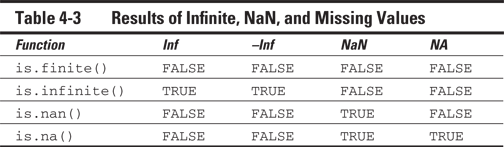
To check whether a value is finite, use the functions is.finite() and is.infinite(). The first function returns TRUE if the number is finite; the second one returns TRUE if the number is infinite. (We discuss the logical values TRUE and FALSE in the next section.)

R considers everything larger than the largest number a computer can hold to be infinity — on most machines, that’s approximately 1.8 × 10308. This definition of infinity can lead to unexpected results, as shown in the following example:

> is.finite(10^(305:310))

[1]  TRUE  TRUE  TRUE  TRUE FALSE FALSE

What does this line of code mean now? See whether you understand the nesting and vectorization in this example. If you break up the line starting from the inner parentheses, it becomes comprehensible:

You know already that 305:310 gives you a vector, containing the integers from 305 to 310.

All operators are vectorized, so 10^(305:310) gives you a vector with the results of 10 to the power of 305, 306, 307, 308, 309, and 310.

That vector is given as an argument to is.finite(). That function tells you that the two last results — 10^308 and 10^309 — are infinite for R.

Dealing with undefined outcomes

Your math teacher probably explained that if you divide any real number by infinity, you get zero. But what if you divide infinity by infinity?

> Inf / Inf

[1] NaN

Well, R tells you that the outcome is NaN. That result simply means Not a Number. This is R’s way of telling you that the outcome of that calculation is not defined.

The funny thing is that R actually considers NaN to be numeric, so you can use NaN in calculations. The outcome of those calculations is always NaN, though, as you see here:

> NaN + 4

[1] NaN

You can test whether a calculation results in NaN by using the is.nan() function. Note that both is.finite() and is.infinite() return FALSE when you’re testing on a NaN value.

Dealing with missing values

As we mention earlier in this chapter, one of the most common problems in statistics is incomplete data sets. To deal with missing values, R uses the reserved keyword NA, which stands for Not Available. You can use NA as a valid value, so you can assign it as a value as well:

> x <- NA

You have to take into account, however, that calculations with a value of NA also generally return NA as a result:

> x + 4

[1] NA

> log(x)

[1] NA

If you want to test whether a value is NA, you can use the is.na() function, as follows:

> is.na(x)

[1] TRUE

Note that the is.na() function also returns TRUE if the value is NaN. The functions is.finite(), is.infinite(), and is.nan() return FALSE for NA values.

Calculating infinite, undefined, and missing values

Table 4-3 provides an overview of results from the functions described in the preceding sections.

Organizing Data in Vectors

Vectors are the most powerful features of R, and in this section, you see why and how you use them.

A vector is a one-dimensional set of values, all the same type. It’s the smallest unit you can work with in R. A single value is technically a vector as well — a vector with only one element. In mathematics vectors are almost always used with numerical values, but in R they also can include other types of data, like character strings (see Chapter 5).

Discovering the properties of vectors

Vectors have a structure and a type, and R is a bit sensitive about both. Feeding R the wrong type of vector is like trying to make your cat eat dog food: Something will happen, and chances are that it won’t be what you hoped for. So, you’d better know what vector you have.

Looking at the structure of a vector

R gives you an easy way to look at the structure of any object. This method comes in handy whenever you doubt the form of the result of a function or a script you wrote. To take a peek inside R objects, use the str() function.

The str() function gives you the type and structure of the object.

Take a look at the vector baskets.of.Granny:

> str(baskets.of.Granny)

num [1:6] 12 4 5 6 9 3

R tells you a few things here:

First, it tells you that this is a num (numeric) type of vector.

Next to the vector type, R gives you the dimensions of the vector. This example has only one dimension, and that dimension has indices ranging from 1 to 6.

Finally, R gives you the first few values of the vector. In this example, the vector has only six values, so you see all of them.

If you want to know only how long a vector is, you can simply use the length() function, as follows:

> length(baskets.of.Granny)

[1] 6

Vectors in R can have other types as well. If you look at the vector authors, for example (refer to Chapter 3), you see a small difference:

> authors <- c(“Andrie”, “Joris”)

> str(authors)

chr [1:2] “Andrie” “Joris”

Again, you get the dimensions, the range of the indices, and the values. But this time, R tells you the type of vector is chr, or character.

In this book, we discuss the following types of vectors:

Numeric vectors, containing all kind of numbers.

Integer vectors, containing integer values. (An integer vector is a special kind of numeric vector.)

Logical vectors, containing logical values (TRUE and/or FALSE)

Character vectors, containing text

Datetime vectors, containing dates and times in different formats

Factors, a special type of vector to work with categories.

We discuss the first three types in this chapter and character vectors in Chapter 5.

R makes clear distinctions among these types of vectors, partly for reasons of logic. Multiplying two words, for example, doesn’t make sense.

Testing vector types

Apart from the str() function, R contains a set of functions that allow you to test for the type of a vector. All these functions have the same syntax: is, a dot, and then the name of the type.

You can test whether a vector is of type foo by using the is.foo() function. This test works for every type of vector; just replace foo with the type you want to check.

To test whether baskets.of.Granny is a numeric vector, for example, use the following code:

> is.numeric(baskets.of.Granny)

[1] TRUE

You may think that baskets.of.Granny is a vector of integers, so check it, as follows:

> is.integer(baskets.of.Granny)

[1] FALSE

R disagrees with the math teacher here. Integer has a different meaning for R than it has for us. The result of is.integer() isn’t about the value but about the way the value is stored in memory.

R has two main modes for storing numbers. The standard mode is double. In this mode, every number uses 64 bits of memory. The number also is stored in three parts. One bit indicates the sign of the number, 52 bits represent the decimal part of the number, and the remaining bits represent the exponent. This way, you can store numbers as big as 1.8 × 10308 in only 64 bits. The integer mode takes only 32 bits of memory, and the numbers are represented as binary integers in the memory. So, the largest integer is about 2.1 billion, or, more exactly, 231 – 1. That’s 31 bits to represent the number itself, 1 bit to represent the sign of the number, and –1 because you start at 0.

You should use integers if you want to do exact integer calculations on small integers or if you want to save memory. Otherwise, the mode double works just fine.

You force R to store a number as an integer by adding L after it, as in the following example:

> x <- c(4L,6L)

> is.integer(x)

[1] TRUE

Whatever mode is used to store the value, is.numeric() returns TRUE in both cases.

Creating vectors

To create a vector from a simple sequence of integers, for example, you use the colon operator (:). The code 3:7 gives you a vector with the numbers 3 to 7, and 4:-3 creates a vector with the numbers 4 to –3, both in steps of 1. To make bigger or smaller steps in a sequence, use the seq() function. This function’s by argument allows you to specify the amount by which the numbers should increase or decrease. For a vector with the numbers 4.5 to 2.5 in steps of 0.5, for example, you can use the following code:

> seq(from = 4.5, to = 2.5, by = -0.5)

[1] 4.5 4.0 3.5 3.0 2.5

Alternatively, you can specify the length of the sequence by using the argument length.out. R calculates the step size itself. You can make a vector of nine values going from –2.7 to 1.3 like this:

> seq(from = -2.7, to = 1.3, length.out = 9)

[1] -2.7 -2.2 -1.7 -1.2 -0.7 -0.2  0.3  0.8  1.3

You don’t have to write out the argument names if you give the values for the arguments in the correct order. The code seq(4.5, 2.5, - 0.5) does exactly the same things as seq(from = 4.5, to = 2.5, by = -0.5). If you use the argument length.out, you always have to be spell it out though.

To get back to our All-Star Grannies example (refer to “Using arithmetic operators,” earlier in this chapter), you have two vectors containing the number of baskets that Granny and her friend Geraldine scored in the six games of this basketball season:

> baskets.of.Granny <- c(12,4,4,6,9,3)

> baskets.of.Geraldine <- c(5,3,2,2,12,9)

Now, what is this c() function doing? To find out, read on.

Combining vectors

The c() function stands for concatenate. It doesn’t create vectors — it just combines them.

In the preceding examples, you give six values as arguments to the c() function and get one combined vector in return. As you know, each value is a vector with one element for R. You also can use the c() function to combine vectors with more than one value, as in the following example:

> all.baskets <-c(baskets.of.Granny, baskets.of.Geraldine)

> all.baskets

[1] 12  4  4  6  9  3  5  3  2  2 12  9

The result of this code is a vector with all 12 values.

In this code, the c() function maintains the order of the numbers. This example illustrates a second important feature of vectors: Vectors have an order. This order turns out to be very useful when you need to manipulate the individual values in the vector, as you do in “Getting Values in and out of Vectors,” later in this chapter.

Repeating vectors

You can combine a vector with itself if you want to repeat it, but if you want to repeat the values in a vector many times, using the c() function becomes a bit impractical. R makes life easier by offering you a function for repeating a vector: rep().

You can use the rep() function in several ways. If you want to repeat the complete vector, for example, you specify the argument times. To repeat the vector c(0, 0, 7) three times, use this code:

> rep(c(0, 0, 7), times = 3)

[1] 0 0 7 0 0 7 0 0 7

You also can repeat every value by specifying the argument each, like this:

> rep(c(2, 4, 2), each = 3)

[1] 2 2 2 4 4 4 2 2 2

R has a little trick up its sleeve. You can tell R for each value how often it has to be repeated. To take advantage of that magic, tell R how often to repeat each value in a vector by using the times argument:

> rep(c(0, 7), times = c(4,2))

[1] 0 0 0 0 7 7

And you can, like in seq, use the argument length.out to tell R how long you want it to be. R will repeat the vector until it reaches that length, even if the last repetition is incomplete, like so:

> rep(1:3,length.out=7)

[1] 1 2 3 1 2 3 1

Getting Values in and out of Vectors

Vectors would be pretty impractical if you couldn’t look up and manipulate individual values. You can perform these tasks easily by using R’s advanced, powerful indexing system.

Understanding indexing in R

Every time R shows you a vector, it displays a number such as [1] in front of the output. In this example, [1] tells you where the first position in your vector is. This number is called the index of that value. If you make a longer vector — say, with the numbers from 1 to 30 — you see more indices. Consider this example:

> numbers <- 30:1

> numbers

[1] 30 29 28 27 26 25 24 23 22 21 20 19 18 17 16 15 14

[18] 13 12 11 10  9  8  7  6  5  4  3  2  1

Here, you see that R counts 13 as the 18th value in the vector. At the beginning of every line, R tells you the index of the first value in that line.

If you try this example on your computer, you may see a different index at the beginning of the line, depending on the width of your console.

Extracting values from a vector

Those brackets ([]) illustrate another strong point of R. They represent a function that you can use to extract a value from that vector. You can get the fifth value of the preceding number vector like this:

> numbers[5]

[1] 26

Okay, this example isn’t too impressive, but the bracket function takes vectors as arguments. If you want to select more than one number, you can simply provide a vector of indices as an argument inside the brackets, like so:

> numbers[c(5,11,3)]

[1] 26 20 28

R returns a vector with the numbers in the order you asked for. So, you can use the indices to order the values the way you want.

You also can store the indices you want to retrieve in another vector and give that vector as an argument, as in the following example:

> indices <- c(5,11,3)

> numbers[indices]

[1] 26 20 28

You can use indices to drop values from a vector as well. If you want all the numbers except for the third value, you can do that with the following code:

> numbers[-3]

[1] 30 29 27 26 25 24 23 22 21 20 19 18 17 16 15 14 13

[18] 12 11 10  9  8  7  6  5  4  3  2  1

Here, too, you can use a complete vector of indices. If you want to expel the first 20 numbers, use this code:

> numbers[-(1:20)]

[1] 10  9  8  7  6  5  4  3  2  1

Be careful to add parentheses around the sequence. If you don’t, R will interpret that as meaning the sequence from –1 to 20, which isn’t what you want here. If you try that code, you get the following error message:

> numbers[-1:20]

Error in numbers[-1:20] : only 0’s may be mixed with negative subscripts

This message makes you wonder what the index 0 is. Well, it’s literally nothing. If it’s the only value in the index vector, you get an empty, or zero-length, vector back, whatever sign you give it; otherwise, it won’t have any effect.

You can’t mix positive and negative index values, so either select a number of values or drop them.

You can do a lot more with indices — they help you write concise and fast code, as we show you in the following sections and chapters.

Changing values in a vector

Let’s get back to the All-Star Grannies. In the previous sections, you created two vectors containing the number of baskets that Granny and Geraldine made in six basketball games.

But suppose that Granny tells you that you made a mistake: In the third game, she made five baskets, not four. You can easily correct this mistake by using indices, as follows:

> baskets.of.Granny[3] <- 5

> baskets.of.Granny

[1] 12  4  5  6  9  3

The assignment to a specific index is actually a function as well. It’s different, however, from the brackets function (refer to “Extracting values from a vector,” earlier in this chapter), because you also give the replacement values as an argument. Boring technical stuff, you say? Not if you realize that because the index assignment is a vectorized function, you can use recycling!

Imagine that you made two mistakes in the number of baskets that Granny’s friend Geraldine scored: She actually scored four times in the second and fourth games. To correct the baskets for Geraldine, you can use the following code:

> baskets.of.Geraldine[c(2,4)] <- 4

> baskets.of.Geraldine

[1]  5  4  2  4 12  9

How cool is that? You have to be careful, though. R doesn’t tell you when it’s recycling values, so a typo may give you unexpected results. Later in this chapter, you find out more about how recycling actually works.

R doesn’t have an Undo button, so when you change a vector, there’s no going back. You can prevent disasters by first making a copy of your object and then changing the values in the copy, as shown in the following example. First, make a copy by assigning the vector baskets.of.Granny to the object Granny.copy:

> Granny.copy <- baskets.of.Granny

You can check what’s in both objects by typing the name on the command line and pressing Enter. Now you can change the vector baskets.of.Granny:

> baskets.of.Granny[4] <- 11

> baskets.of.Granny

[1] 12  4  5 11  9  3

If you make a mistake, simply assign the vector Granny.copy back to the object baskets.of.Granny, like this:

> baskets.of.Granny <- Granny.copy

> baskets.of.Granny

[1] 12  4  5  6  9  3

Working with Logical Vectors

Up to now, we haven’t really discussed the values TRUE and FALSE. For some reason, the developers of R decided to call these values logical values. In other programming languages, TRUE and FALSE are known as Boolean values. As Shakespeare would ask, what’s in a name? Whatever name they go by, these values come in handy when you start controlling the flow of your scripts, as we discuss in Chapter 9.

You can do a lot more with these values, however, because you can construct vectors that contain only logical values — the logical vectors that we mention in “Looking at the structure of a vector,” earlier in this chapter. You can use these vectors as an argument for the index functions, which makes for a powerful tool.

Comparing values

To build logical vectors, you’d better know how to compare values, and R contains a set of operators that you can use for this purpose (see Table 4-4).

Table 4-4 Comparing Values in R

Operator	Result
x == y	Returns TRUE if x exactly equals y
x != y	Returns TRUE if x differs from y
x > y	Returns TRUE if x is larger than y
x >= y	Returns TRUE if x is larger than or exactly equal to y
x < y	Returns TRUE if x is smaller than y
x <= y	Returns TRUE if x is smaller than or exactly equal to y
x & y	Returns the result of x and y
x | y	Returns the result of x or y
! x	Returns not x
xor( x, y )	Returns the result of x xor y (x or y but not x and y)

All these operators are, again, vectorized. You can compare a whole vector with a value. In the continuing All-Star Grannies example, to find out which games Granny scored more than five baskets in, you can simply use this code:

> baskets.of.Granny > 5

[1]  TRUE FALSE FALSE  TRUE  TRUE FALSE

You can see that the result is the first, fourth, and fifth games. This example works well for small vectors like this one, but if you have a very long vector, counting the number of games would be a hassle. For that purpose, R offers the delightful which() function. To find out which games Granny scored more than five baskets in, you can use the following code:

> which(baskets.of.Granny > 5)

[1] 1 4 5

With this one line of code, you actually do two different things: First, you make a logical vector by checking every value in the vector to see whether it’s greater than five. Then you pass that vector to the which() function, which returns the indices in which the value is TRUE.

The which() function takes a logical vector as argument. Hence, you can save the outcome of a logical vector in an object and pass that to the which() function, as in the next example. You also can use all these operators to compare vectors value by value. You can easily find out the games in which Geraldine scored fewer baskets than Granny like this:

> the.best <- baskets.of.Geraldine < baskets.of.Granny

> which(the.best)

[1] 1 3 4

Always put spaces around the less than (<) and greater than (>) operators. Otherwise, R may mistake x < -3 for the assignment x <- 3. The difference may seem small, but it has a huge effect on the result. Technically, you also can use the equal sign (=) as an assignment to prevent this problem, but = also is used to assign values to arguments in functions. In general, <- is the preferred way to assign a value to an object, but quite a few coders disagree. So, it’s up to you. We use <- in this book.

Using logical vectors as indices

The index function doesn’t take only numerical vectors as arguments; it also works with logical vectors. You can use these logical vectors very efficiently to select some values from a vector. If you use a logical vector to index, R returns a vector with only the values for which the logical vector is TRUE.

In the preceding section, a logical vector, the.best, tells you the games in which Granny scored more than Geraldine did. If you want to know how many baskets Granny scored in those games, you can use this code:

> baskets.of.Granny[the.best]

[1] 12  5  6

This construct is often used to keep only values that fulfill a certain requirement. If you want to keep only the values larger than 2 in the vector x, you could do that with the following code:

> x <- c(3, 6, 1, NA, 2)

> x[x > 2]

[1]  3  6 NA

Wait — what is that NA value doing there? Take a step back, and look at the result of x > 2:

> x > 2

[1]  TRUE  TRUE FALSE    NA FALSE

If you have a missing value in your vector, any comparison returns NA for that value (refer to “Dealing with missing values,” earlier in this chapter).

It may seem that this NA is translated into TRUE, but that isn’t the case. If you give NA as a value for the index, R puts NA in that place as well. So, in this case, R keeps the first and second values of x, drops the third, adds one missing value, and drops the last value of x as well.

Combining logical statements

Life would be boring if you couldn’t combine logical statements. If you want to test whether a number lies within a certain interval, for example, you want to check whether it’s greater than the lowest value and less than the top value. Maybe you want to know the games in which Granny scored the fewest or the most baskets. For that purpose, R has a set of logical operators that — you guessed it — are nicely vectorized (refer to Table 4-4).

To illustrate, using the knowledge you have now, try to find out the games in which Granny scored the fewest baskets and the games in which she scored the most baskets:

1. Create two logical vectors, as follows:

> min.baskets <- baskets.of.Granny == min(baskets.of.Granny)

> max.baskets <- baskets.of.Granny == max(baskets.of.Granny)

min.baskets tells you whether the value is equal to the minimum, and max.baskets tells you whether the value is equal to the maximum.

2. Combine both vectors with the OR operator (|), as follows:

> min.baskets | max.baskets

[1]  TRUE FALSE FALSE FALSE FALSE  TRUE

This method actually isn’t the most efficient way to find those values. You see how to do things like this more efficiently with the match() function in Chapter 13. But this example clearly shows you how vectorization works for logical operators.

The NOT operator (!) is another example of the great power of vectorization. The NA values in the vector x have caused some trouble already, so you’d probably like to get rid of them. You know from “Dealing with undefined outcomes,” earlier in this chapter, that you have to check whether a value is missing by using the is.na() function. But you need the values that are not missing values, so invert the logical vector by preceding it with the ! operator. To drop the missing values in the vector x, for example, use the following code:

> x[!is.na(x)]

[1] 3 6 2 1

When you’re using R, there’s no way to get around vectorization. After you understand how vectorization works, however, you’ll save considerable calculation time and lines of code.

Summarizing logical vectors

You also can use logical values in arithmetic operations as well. In that case, R sees TRUE as 1 and FALSE as 0. This allows for some pretty interesting constructs.

Suppose that you’re not really interested in finding out the games in which Granny scored more than Geraldine did, but you want to know how often that happened. You can use the numerical translation of a logical vector for that purpose in the sum() function, as follows:

> sum(the.best)

[1] 3

So, three times, Granny was better than Geraldine. Granny rocks!

In addition, you have an easy way to figure out whether any value in a logical vector is TRUE. Very conveniently, the function that performs that task is called any(). To ask R whether Granny was better than Geraldine in any game, use this code:

> any(the.best)

[1] TRUE

We told you that Granny rocks! Well, okay, this result is a bit unfair for Geraldine, so you should check whether Granny was better than Geraldine in all the games. The R function you use for this purpose is called — surprise, surprise — all(). To find out whether Granny was always better than Geraldine, use the following code:

> all(the.best)

[1] FALSE

Still, Granny rocks a bit.

You can use the argument na.rm=TRUE in the functions all() and any() as well. By default, both functions return NA if any value in the vector argument is missing (see “Dealing with missing values,” earlier in this chapter).

Powering Up Your Math with Vector Functions

As we suggest throughout this chapter, vectorization is the Holy Grail for every R programmer. Most beginners struggle a bit with that concept because vectorization isn’t one little trick, but a way of coding. Using the indices and vectorized operators, however, can save you a lot of coding and calculation time — and then you can call a gang of power functions to work on your data, as we show you in this section.

Why are power functions so helpful? Maybe you’re like us: We’re lazy and impatient enough to try to translate our code into “something with vectors” as often as possible. We don’t like to type too much, and we definitely don’t like to wait for the results. If you can relate, read on.

Using arithmetic vector operations

A third set of arithmetic functions consists of functions in which the outcome is dependent on more than one value in the vector. Summing a vector with the sum() function is such an operation. You find an overview of the most important functions in Table 4-5.

Table 4-5 Vector Operations

Function	What It Does
sum(x)	Calculates the sum of all values in x
prod(x)	Calculates the product of all values in x
min(x)	Gives the minimum of all values in x
max(x)	Gives the maximum of all values in x
cumsum(x)	Gives the cumulative sum of all values in x
cumprod(x)	Gives the cumulative product of all values in x
cummin(x)	Gives the minimum for all values in x from the start of the vector until the position of that value
cummax(x)	Gives the maximum for all values in x from the start of the vector until the position of that value
diff(x)	Gives for every value the difference between that value and the next value in the vector

Summarizing a vector

You can tell quite a few things about a set of values with one number. If you want to know the minimum and maximum number of baskets Granny made, for example, you use the functions min() and max():

> min(baskets.of.Granny)

[1] 3

> max(baskets.of.Granny)

[1] 12

To calculate the sum and the product of all values in the vector, use the functions sum() and prod(), respectively.

These functions also can take a list of vectors as an argument. If you want to calculate the sum of all the baskets made by Granny and Geraldine, you can use the following code:

> sum(baskets.of.Granny,baskets.of.Geraldine)

[1] 75

The same works for the other vector operations in this section.

As we discuss in “Dealing with missing values,” earlier in this chapter, missing values always return NA as a result. The same is true for vector operations as well. R, however, gives you a way to simply discard the missing values by setting the argument na.rm to TRUE. Take a look at the following example:

> x <- c(3,6,2,NA,1)

> sum(x)

[1] NA

> sum(x,na.rm=TRUE)

[1] 12

This argument works in sum(), prod(), min(), and max().

If you have a vector that contains only missing values and you set the argument na.rm to TRUE, the outcome of these functions is set in such a way that it doesn’t have any effect on further calculations. The sum of missing values is 0, the product is 1, the minimum is Inf, and the maximum is -Inf. R won’t always generate a warning in such a case, though. Only in the case of min() and max() does R tell you that there were no non-missing arguments.

Cumulating operations

Suppose that after every game, you want to update the total number of baskets that Granny made during the season. After the second game, that’s the total of the first two games; after the third game, it’s the total of the first three games; and so on. You can make this calculation easily by using the cumulative sum function, cumsum(), as in the following example:

> cumsum(baskets.of.Granny)

[1] 12 16 21 27 36 39

In a similar way, cumprod() gives you the cumulative product. You also can get the cumulative minimum and maximum with the related functions cummin() and cummax(). To find the maximum number of baskets Geraldine scored up to any given game, you can use the following code:

> cummax(baskets.of.Geraldine)

[1]  5  5  5  5 12 12

These functions don’t have an extra argument to remove missing values. Missing values are propagated through the vector, as shown in the following example:

> cummin(x)

[1]  3  3  2 NA NA

Calculating differences

The last function we’ll discuss in this section calculates differences between adjacent values in a vector. You can calculate the difference in the number of baskets between every two games Granny played by using the following code:

> diff(baskets.of.Granny)

[1] -8  1  1  3 -6

You get five numbers back. The first one is the difference between the first and the second game, the second is the difference between the second and the third game, and so on.

The vector returned by diff() is always one element shorter than the original vector you gave as an argument.

The rule about missing values applies here, too. When your vector contains a missing value, the result from that calculation will be NA. So, if you calculate the difference with the vector x, you get the following result:

> diff(x)

[1]  3 -4 NA NA

Because the fourth element of x is NA, the difference between the third and fourth element and between the fourth and fifth element will be NA as well. Just like the cumulative functions, the diff() function doesn’t have an argument to eliminate the missing values.

Recycling arguments

In Chapter 3 and earlier in this chapter, we mention recycling arguments. Take a look again at how you calculate the total amount of money Granny and Geraldine raised (see “Using arithmetic operators,” earlier in this chapter) or how you combine the first names and last names of three siblings (see Chapter 3). Each time, you combine a vector with multiple values and one with a single value in a function. R applies the function, using that single value for every value in the vector. But recycling goes far beyond these examples.

Any time you give two vectors with unequal lengths to a recycling function, R repeats the shortest vector as often as necessary to carry out the task you asked it to perform. In the earlier examples, the shortest vector is only one value long.

Suppose you split up the number of baskets Granny made into two-pointers and three-pointers:

> Granny.pointers <- c(10,2,4,0,4,1,4,2,7,2,1,2)

You arrange the numbers in such a way that for every game, first the number of two-pointers is given, followed by the number of three-pointers.

Now Granny wants to know how many points she’s actually scored this season. You can calculate that easily with the help of recycling:

> points <- Granny.pointers * c(2,3)

> points

[1] 20  6  8  0  8  3  8  6 14  6  2  6

> sum(points)

[1] 87

Now, what did you do here?

1. You made a vector with the number of points for each basket:

c(2,3)

2. You told R to multiply that vector by the vector Granny.pointers.

R multiplied the first number in Granny.pointers by 2, the second by 3, the third by 2 again, and so on.

3. You put the result in the variable points.

4. You summed all the numbers in points to get the total number of points scored.

In fact, you can just leave out Step 3. The nesting of functions allows you to do this in one line of code:

> sum(Granny.pointers * c(2,3))

Recycling can be a bit tricky. If the length of the longer vector isn’t exactly a multiple of the length of the shorter vector, you can get unexpected results.

Now Granny wants to know how much she improved every game. Being lazy, you have a cunning plan. With diff(), you calculate how many more or fewer baskets Granny made than she made in the game before. Then you use the vectorized division to divide these differences by the number of baskets in the game. To top it off, you multiply by 100 and round the whole vector. All these calculations take one line of code:

> round(diff(baskets.of.Granny) / baskets.of.Granny * 100 )

1st  2nd  3rd  4th  5th  6th

-67   25   20   50  -67 -267

That last value doesn’t look right, because it’s impossible to score more than 100 percent fewer baskets. R doesn’t just give you that weird result; it also warns you that the length of diff(baskets.of.Granny) doesn’t fit the length of baskets.of.Granny:

Warning message:

In diff(baskets.of.Granny)/baskets.of.Granny :

  longer object length is not a multiple of shorter object length

The vector baskets.of.Granny is six values long, but the outcome of diff(baskets.of.Granny) is only five values long. So the decrease of 267 percent is, in fact, the last value of baskets.of.Granny divided by the first value of diff(baskets.of.Granny). In this example, the shortest vector, diff(baskets.of.Granny), gets recycled by the division operator.

That result wasn’t what you intended. To prevent that outcome, you should use only the first five values of baskets.of.Granny, so the length of both vectors match:

> round(diff(baskets.of.Granny) / baskets.of.Granny[1:5] * 100)

2nd 3rd 4th 5th 6th

-67  25  20  50 -67

And all that is vectorization.