
Figure 15-1: Plotting histograms for different groups.
Chapter 15
Testing Differences and Relations
In This Chapter
![]() Evaluating distributions
Evaluating distributions
![]() Comparing two samples
Comparing two samples
![]() Comparing more than two samples
Comparing more than two samples
![]() Testing relations between categorical variables
Testing relations between categorical variables
![]() Working with models
Working with models
It’s one thing to describe your data and plot a few graphs, but if you want to draw conclusions from these graphs, people expect a bit more proof. This is where the data analysts chime in and start pouring p-values generously over reports and papers. These p-values summarize the conclusions of statistical tests, basically indicating how likely it is that the result you see is purely due to chance. The story is a bit more complex — but for that you need to take a look at a statistics handbook like Statistics For Dummies, 2nd Edition, by Deborah J. Rumsey, PhD (Wiley).
R really shines when you need some serious statistical number crunching. Statistics is the alpha and omega of this language, but why have we waited until Chapter 15 to cover some of that? There are two very good reasons why we wait to talk about statistics until now:
![]() You can start with the statistics only after you’ve your data in the right format, so you need to get that down first.
You can start with the statistics only after you’ve your data in the right format, so you need to get that down first.
![]() R contains an overwhelming amount of advanced statistical techniques, many of which come with their own books and manuals.
R contains an overwhelming amount of advanced statistical techniques, many of which come with their own books and manuals.
Luckily, many packages follow the same principles regarding the user interface. So, instead of trying to cover all of what’s possible, in this chapter we introduce you to some basic statistical tests and explain the interfaces in more detail so you get familiar with that.
Taking a Closer Look at Distributions
The normal distribution (also known as the Gaussian distribution or bell curve) is a key concept in statistics. Much statistical inference is based on the assumption that, at some point in your calculations, you have values that are distributed normally. Testing whether the distribution of your data follows this bell curve closely enough is often one of the first things you do before you choose a test to test your hypothesis.
 If you’re not familiar with the normal distribution, check out Statistics For Dummies, 2nd Edition, by Deborah J. Rumsey, PhD (Wiley), which devotes a whole chapter to this concept.
Observing beavers
Let’s take a look at an example. The biologist and statistician Penny Reynolds observed some beavers for a complete day and measured their body temperature every ten minutes. She also wrote down whether the beavers were active at that moment. You find the measurements for one of these animals in the dataset beavers, which consists of two data frames; for the examples, we use the second one, which contains only four variables, as you can see in the following:
> str(beaver2)
‘data.frame’: 100 obs. of 4 variables:
$ day : num 307 307 307 307 307 ...
$ time : num 930 940 950 1000 1010 ...
$ temp : num 36.6 36.7 ...
$ activ: num 0 0 0 0 0 ...
If you want to know whether there’s a difference between the average body temperature during periods of activity and periods without, you first have to choose a test. To know which test is appropriate, you need to find out if the temperature is distributed normally during both periods. So, let’s take a closer look at the distributions.
Testing normality graphically
You could, of course, plot a histogram for every sample you want to look at. You can use the histogram() function pretty easily to plot histograms for different groups. (This function is part of the lattice package you use in Chapter 17.)
Using the formula interface, you can plot two histograms in Figure 15-1 at once using the following code:
> library(lattice)
> histogram(~temp | factor(activ), data=beaver2)

You find more information about the formula interface in Chapter 13, but let’s go over this formula once more. The histogram() function uses a one-sided formula, so you don’t specify anything at the left side of the tilde (~). On the right side, you specify the following:
![]() Which variable the histogram should be created for: In this case, that’s the variable
Which variable the histogram should be created for: In this case, that’s the variable temp, containing the body temperature.
![]() After the vertical line (
After the vertical line (|),the factor by which the data should be split: In this case, that’s the variable activ that has a value 1 if the beaver was active and 0 if it was not. To convert this numeric variable to a factor, you use the factor() function.
 The vertical line (
|) in the formula interface can be read as “conditional on.” It’s used in that context in the formula interfaces of more advanced statistical functions as well.
Using quantile plots
Still, histograms leave much to the interpretation of the viewer. A better graphical way to tell whether your data is distributed normally is to look at a so-called quantile-quantile (QQ) plot.
With this technique, you plot quantiles against each other. If you compare two samples, for example, you simply compare the quantiles of both samples. Or, to put it a bit differently, R does the following to construct a QQ plot:
![]() It sorts the data of both samples.
It sorts the data of both samples.
![]() It plots these sorted values against each other.
It plots these sorted values against each other.
If both samples don’t contain the same number of values, R calculates extra values by interpolation for the smallest sample to create two samples of the same size.
Comparing two samples
Of course, you don’t have to do that all by yourself, you can simply use the qqplot() function for that. So, to check whether the temperatures during activity and during rest are distributed equally, you simply do the following:
> qqplot(beaver2$temp[beaver2$activ==1],
+ beaver2$temp[beaver2$activ==0])
This creates a plot where the ordered values are plotted against each other, as shown in Figure 15-2. You can use all the tricks from Chapter 16 to change axis titles, color and appearance of the points, and so on.
Figure 15-2: Plotting a QQ plot of two different samples.

 Between the square brackets, you can use a logical vector to select the cases you want. Here you select all cases where the variable
 activ equals 1 for the first sample, and all cases where that variable equals 0 for the second sample.
Using a QQ plot to check for normality
In most cases, you don’t want to compare two samples with each other, but compare a sample with a theoretical sample that comes from a certain distribution (for example, the normal distribution).
To make a QQ plot this way, R has the special qqnorm() function. As the name implies, this function plots your sample against a normal distribution. You simply give the sample you want to plot as a first argument and add any of the graphical parameters from Chapter 16 you like. R then creates a sample with values coming from the standard normal distribution, or a normal distribution with a mean of zero and a standard deviation of one. With this second sample, R creates the QQ plot as explained before.
R also has a qqline() function, which adds a line to your normal QQ plot. This line makes it a lot easier to evaluate whether you see a clear deviation from normality. The closer all points lie to the line, the closer the distribution of your sample comes to the normal distribution. The qqline() function also takes the sample as an argument.
Now you want to do this for the temperatures during both the active and the inactive period of the beaver. You can use the qqnorm() function twice to create both plots. For the inactive periods, you can use the following code:
> qqnorm( beaver2$temp[beaver2$activ==0], main=’Inactive’)
> qqline( beaver2$temp[beaver2$activ==0] )
You can do the same for the active period by changing the value 0 to 1. The resulting plots you see in Figure 15-3.
Figure 15-3: Comparing samples to the normal distribution with QQ plots.

Testing normality in a formal way
All these graphical methods for checking normality still leave much to your own interpretation. There’s much discussion in the statistical world about the meaning of these plots and what can be seen as normal. If you show any of these plots to ten different statisticians, you can get ten different answers. That’s quite an achievement when you expect a simple yes or no, but statisticians don’t do simple answers.
On the contrary, everything in statistics revolves around measuring uncertainty. This uncertainty is summarized in a probability — often called a p-value — and to calculate this probability, you need a formal test.
Probably the most widely used test for normality is the Shapiro-Wilks test. The function to perform this test, conveniently called shapiro.test(), couldn’t be easier to use. You give the sample as the one and only argument, as in the following example:
> shapiro.test(beaver2$temp)
Shapiro-Wilks normality test
data: beaver2$temp
W = 0.9334, p-value = 7.764e-05
This function returns a list object, and the p-value is contained in a element called p.value. So, for example, you can extract the p-value simply by using the following code:
> result <- shapiro.test(beaver2$temp)
> result$p.value
[1] 7.763782e-05
This p-value tells you what the chances are that the sample comes from a normal distribution. The lower this value, the smaller the chance. Statisticians typically use a value of 0.05 as a cutoff, so when the p-value is lower than 0.05, you can conclude that the sample deviates from normality. In the preceding example, the p-value is clearly lower than 0.05 — and that shouldn’t come as a surprise; the distribution of the temperature shows two separate peaks (refer to Figure 15-1). This is nothing like the bell curve of a normal distribution.
When you choose a test, you may be more interested in the normality in each sample. You can test both samples in one line using the tapply() function, like this:
> with(beaver2, tapply(temp, activ, shapiro.test))
This code returns the results of a Shapiro-Wilks test on the temperature for every group specified by the variable activ.
 People often refer to the Kolmogorov-Smirnov test for testing normality. You carry out the test by using the
 ks.test() function in base R. But this R function is not suited to test deviation from normality; you can use it only to compare different distributions.
Comparing Two Samples
Comparing groups is one of the most basic problems in statistics. If you want to know if extra vitamins in the diet of cows is increasing their milk production, you give the normal diet to a control group and extra vitamins to a test group, and then you compare the milk production in two groups. By comparing the mileage between cars with automatic gearboxes and those with manual gearboxes, you can find out which one is the more economical option.
Testing differences
R gives you two standard tests for comparing two groups with numerical data: the t-test with the t.test() function, and the Wilcoxon test with the wilcox.test() function. If you want to use the t.test() function, you first have to check, among other things, whether both samples are normally distributed using any of the methods from the previous section. For the Wilcoxon test, this isn’t necessary.
Carrying out a t-test
Let’s take another look at the data of that beaver. If you want to know if the average temperature differs between the periods the beaver is active and inactive, you can do so with a simple command:
> t.test(temp ~ activ, data=beaver2)
Welch Two-Sample t-test
data: temp by activ
t = -18.5479, df = 80.852, p-value < 2.2e-16
alternative hypothesis: true difference in means is not equal to 0
95 percent confidence interval:
-0.8927106 -0.7197342
sample estimates:
mean in group 0 mean in group 1
37.09684 37.90306
Normally, you can only carry out a t-test on samples for which the variances are approximately equal. R uses Welch’s variation on the t-test, which corrects for unequal variances.
You get a whole lot of information here:
![]() The second line gives you the test statistic (
The second line gives you the test statistic (t for this test), the degrees of freedom (df), and the according p-value. The very small p-value indicates that the means of both samples differ significantly.
![]() The alternative hypothesis tells you what you can conclude if the p-value is lower than the limit for significance. Generally, scientists consider the alternative hypothesis to be true if the p-value is lower than 0.05.
The alternative hypothesis tells you what you can conclude if the p-value is lower than the limit for significance. Generally, scientists consider the alternative hypothesis to be true if the p-value is lower than 0.05.
![]() The 95 percent confidence interval is the interval that contains the difference between the means with 95 percent probability, so in this case the difference between the means lies probably between 0.72 and 0.89.
The 95 percent confidence interval is the interval that contains the difference between the means with 95 percent probability, so in this case the difference between the means lies probably between 0.72 and 0.89.
![]() The last line gives you the means of both samples.
The last line gives you the means of both samples.
You read the formula temp ~ activ as “evaluate temp within groups determined by activ.” Alternatively, you can use two separate vectors for the samples you want to compare and pass both to the function, as in the following example:
> activetemp <- beaver2$temp[beaver2$activ==1]
> inactivetemp <- beaver2$temp[beaver2$activ==0]
> t.test(activetemp, inactivetemp)
Dropping assumptions
In some cases, your data deviates significantly from normality and you can’t use the t.test() function. For those cases, you have the wilcox.test() function, which you use in exactly the same way, as shown in the following example:
> wilcox.test(temp ~ activ, data=beaver2)
This give you the following output:
Wilcoxon rank-sum test with continuity correction
data: temp by activ
W = 15, p-value < 2.2e-16
alternative hypothesis: true location shift is not equal to 0
Again, you get the value for the test statistic (W in this test) and a p-value. Under that information, you read the alternative hypothesis, and that differs a bit from the alternative hypothesis of a t-test. The Wilcoxon test looks at whether the center of your data (the location) differs between both samples.
With this code, you perform the Wilcoxon rank-sum test or Mann-Whitney U test. Both tests are completely equivalent, so R doesn’t contain a separate function for Mann-Whitney’s U test.
Testing direction
In both previous examples, you test whether the samples differ without specifying in which way. Statisticians call this a two-sided test. Imagine you don’t want to know whether body temperature differs between active and inactive periods, but whether body temperature is lower during inactive periods.
To do this, you have to specify the argument alternative in either the t.test() or wilcox.test() function. This argument can take three values:
![]() By default, it has the value
By default, it has the value ‘two.sided’, which means you want the standard two-sided test.
![]() If you want to test whether the mean (or location) of the first group is lower, you give it the value
If you want to test whether the mean (or location) of the first group is lower, you give it the value ‘less’.
![]() If you want to test whether that mean is bigger, you specify the value
If you want to test whether that mean is bigger, you specify the value ‘greater’.
If you use the formula interface for these tests, the groups are ordered in the same order as the levels of the factor you use. You have to take that into account to know which group is seen as the first group. If you give the data for both groups as separate vectors, the first vector is the first group.
Comparing paired data
When testing differences between two groups, you can have either paired or unpaired data. Paired data comes from experiments where two different treatments were given to the same subjects.
For example, researchers gave ten people two variants of a sleep medicine. Each time the researchers recorded the difference in hours of sleep with and without the drugs. Because each person received both variants, the data is paired. You find the data of this experiment in the dataset sleep, which has three variables:
![]() A numeric variable
A numeric variable extra, which give the extra hours of sleep after the medication is taken
![]() A factor variable
A factor variable group that tells which variant the person took
![]() A factor variable
A factor variable id that indicates the ten different test persons
Now they want to know whether both variants have a different effect on the length of the sleep. Both the t.test() and the wilcox.test() functions have an argument paired that you can set to TRUE in order to carry out a test on paired data. You can test differences between both variances using the following code:
> t.test(extra ~ group, data=sleep, paired=TRUE)
This gives you the following output:
Paired t-test
data: extra by group
t = -4.0621, df = 9, p-value = 0.002833
alternative hypothesis: true difference in means is not equal to 0
95 percent confidence interval:
-2.4598858 -0.7001142
sample estimates:
mean of the differences
-1.58
Unlike the unpaired test, you don’t get the means of both groups; instead, you get a single mean of the differences.
Testing Counts and Proportions
Many research questions revolve around counts instead of continuous numerical measurements. Counts can be summarized in tables and subsequently analyzed. In the following section, you use some of the basic tests for counts and proportions contained in R. Be aware, though, that this is just the tip of the iceberg; R has a staggering amount of statistical procedures for categorical data available.
If you need more background on the statistics, check the book Categorical Data Analysis, 2nd Edition, by Alan Agresti (Wiley-Interscience). In addition, Jana Thompson wrote a manual with R code to illustrate all the examples in Agresti’s book; you can download it on her website at https://home. comcast.net/~lthompson221/Splusdiscrete2.pdf.
Checking out proportions
Let’s look at an example to illustrate the basic tests for proportions.
The following example is based on real research, published by Robert Rutledge, MD, and his colleagues in the Annals of Surgery (1993).
In a hospital in North Carolina, the doctors registered the patients who were involved in a car accident and whether they used seat belts. The following matrix represents the number of survivors and deceased patients in each group:
> survivors <- matrix(c(1781,1443,135,47), ncol=2)
> colnames(survivors) <- c(‘survived’,’died’)
> rownames(survivors) <- c(‘no seat belt’,’seat belt’)
> survivors
survived died
no seat belt 1781 135
seat belt 1443 47
To know whether seat belts made a difference in the chances of surviving, you can carry out a proportion test. This test tells how probable it is that both proportions are the same. A low p-value tells you that both proportions probably differ from each other. To test this in R, you can use the prop.test() function on the preceding matrix:
> result.prop <- prop.test(survivors)
You also can use the prop.test() function on tables or vectors. If you use it with vectors, remember that the first vector has to be the number of successes, and the second number has to be the total number of cases.
The prop.test() function then gives you the following output:
> result.prop
2-sample test for equality of proportions with continuity correction
data: survivors
X-squared = 24.3328, df = 1, p-value = 8.105e-07
alternative hypothesis: two.sided
95 percent confidence interval:
-0.05400606 -0.02382527
sample estimates:
prop 1 prop 2
0.9295407 0.9684564
This test report is almost identical to the one from t.test() and contains essentially the same information. At the bottom, R prints for you the proportion of people who died in each group. The p-value tells you how likely it is that both the proportions are equal. So, you see that the chance of dying in a hospital after a crash is lower if you’re wearing a seat belt at the time of the crash. R also reports the confidence interval of the difference between the proportions.
Analyzing tables
You can use the prop.test() function for matrices and tables. For prop.test(), these tables need to have two columns with the number of counts for the two possible outcomes like the matrix survivors from the previous section.
Testing contingency of tables
Alternatively, you can use the chisq.test() function to analyze tables with a chi-squared (χ2) contingency test. To do this on the matrix with the seat-belt data, you simply do the following:
> chisq.test(survivors)
This returns the following output:
Pearson’s Chi-squared test with Yates’ continuity correction
data: survivors
X-squared = 24.3328, df = 1, p-value = 8.105e-07
The values for the statistic (X-squared), the degrees of freedom, and the p-value are exactly the same as with the prop.test() function. That’s to be expected, because — in this case, at least — both tests are equivalent.
Testing tables with more than two columns
Unlike the prop.test() function, the chisq.test() function can deal with tables with more than two columns and even with more than two dimensions. To illustrate this, let’s take a look at the table HairEyeColor. You can see its structure with the following code:
> str(HairEyeColor)
table [1:4, 1:4, 1:2] 32 53 10 3 11 50 10 30 10 25 ...
- attr(*, “dimnames”)=List of 3
..$ Hair: chr [1:4] “Black” “Brown” “Red” “Blond”
..$ Eye : chr [1:4] “Brown” “Blue” “Hazel” “Green”
..$ Sex : chr [1:2] “Male” “Female”
So, the table HairEyeColor has three dimensions: one for hair color, one for eye color, and one for sex. The table represents the distribution of these three features among 592 students.
The dimension names of a table are stored in an attribute called dimnames. As you can see from the output of the str() function, this is actually a list with the names for the rows/columns in each dimension. If this list is a named list, the names are used to label the dimensions. You can use the dimnames() function to extract or change the dimension names. (Go to the Help page ?dimnames for more examples.)
To check whether hair color and eye color are related, you can collapse the table over the first two dimensions using the margin.table() function to summarize hair and eye color for both genders. This function sums the values in some dimensions to give you a summary table with fewer dimensions. For that, you have to specify which margins you want to keep.
So, to get the table of hair and eye color, you use the following:
> HairEyeMargin <- margin.table(HairEyeColor, margin=c(1,2))
> HairEyeMargin
Eye
Hair Brown Blue Hazel Green
Black 68 20 15 5
Brown 119 84 54 29
Red 26 17 14 14
Blond 7 94 10 16
Now you can simply check whether hair and eye color are related by testing it on this table:
> chisq.test(HairEyeMargin)
Pearson’s Chi-squared test
data: HairEyeMargin
X-squared = 138.2898, df = 9, p-value < 2.2e-16
As expected, the output of this test tells you that some combinations of hair and eye color are more common than others. Not a big surprise, but you can use these techniques on other, more interesting research questions.
Extracting test results
Many tests in this chapter return a htest object. That type of object is basically a list with all the information about the test that has been carried out. All these htest objects contain at least an element statistic with the value of the statistic and an element p.value with the value of the p-value. You can see this easily if you look at the structure of the returned object. The object returned by shapiro.test() in the previous section looks like this:
> str(result)
List of 4
$ statistic: Named num 0.933
..- attr(*, “names”)= chr “W”
$ p.value : num 7.76e-05
$ method : chr “Shapiro-Wilk normality test”
$ data.name: chr “beaver2$temp”
- attr(*, “class”)= chr “htest”
Because this htest objects are lists, you can use any of the list subsetting methods to extract the information. The following code, for example, extracts the p-value from the t-test on the beaver data:
> t.test(temp ~ activ, data=beaver2)$p.value
[1] 7.269112e-31
The extraction of information from the htest object also works with the results of the other .test functions in this chapter and many more. You can check what kind of object a test returns by looking at the Help page for the test you want to use.
Working with Models
The tests we describe in the previous sections are all basic statistical tests. However, these days, much of statistics involves working with complex models. Base R already contains an extensive set of modeling tools, allowing you to do anything from simple linear models and analysis of variance to mixed models and time-series analysis. The nice thing about modeling functions in R is that they often work in a similar way.
Because this isn’t a statistics book, we can’t cover the details about assumption testing and model evaluation. If you aren’t familiar with these concepts or the applied models, be sure to consult a decent source of information, or you’ll run the risk of basing important decisions on inadequate models. The book Applied Linear Statistical Models, 5th Edition, by Michael Kutner et al (McGraw-Hill/Irwin), is very extensive but gives a good and thorough theoretical introduction on assumption testing and model evaluation.
In this section, we cover some basic models, and show you how to extract useful information from the resulting model objects.
Analyzing variances
An analysis of variance (ANOVA) is a very common technique used to compare the means between different groups. To illustrate this, take a look at the dataset InsectSpray:
> str(InsectSprays)
‘data.frame’: 72 obs. of 2 variables:
$ count: num 10 7 20 14 14 12 10 23 17 20 ...
$ spray: Factor w/ 6 levels “A”,”B”,”C”,”D”,..: 1 1 1 1 1 1 1 1 1 1 ...
This dataset contains the results of an agricultural experiment. Six insecticides were tested on 12 fields each, and the researchers counted the number of pesky bugs that remained on each field. Now the farmers need to know if the insecticides make any difference, and if so, which one they best use. You answer this question by using the aov() function to perform an ANOVA.
Building the model
For this simple example, building the model is a piece of cake. You essentially want to model the means for the variable count as a function of the variable spray. You translate that to R like this:
> AOVModel <- aov(count ~ spray, data=InsectSprays)
You pass two arguments to the aov() function in this line of code:
![]() The formula
The formula count ~ spray, which reads as “count as a function of spray”
![]() The argument
The argument data, where you specify the data frame in which the variables in the formula can be found
Every modeling function returns a model object with a lot of information about the fitted model. Always put this model object in a variable. This way you don’t have to refit the model when you need to perform extra calculations.
Looking at the object
As with every object, you can look at a model object just by typing its name in the console. If you do that for the object Model that you created in the preceding section, you see the following output:
> AOVModel
Call:
aov(formula = count ~ spray, data=InsectSprays)
Terms:
spray Residuals
Sum of Squares 2668.833 1015.167
Deg. of Freedom 5 66
Residual standard error: 3.921902
Estimated effects may be unbalanced
This doesn’t tell you that much, apart from the command (or the call) you used to build the model and some basic information on the fitting result.
In the output, you also read that the estimated effects may be unbalanced. This isn’t a warning as described in Chapter 10 — it’s a message that’s built in by the author of the aov() function. This one can pop up in two situations:
![]() You don’t have the same number of cases in every group.
You don’t have the same number of cases in every group.
![]() You didn’t set orthogonal contrasts.
You didn’t set orthogonal contrasts.
In this case, it’s the second reason. You can continue with this model as we do now (that’s also how those models are fitted in SPSS and SAS by default) or you can read the nearby sidebar, “Setting the contrasts,” and use contrasts as the statistical experts who wrote R think you should.
Evaluating the differences
To check the model, you can use the summary() function on the model object like this:
> summary(AOVModel)
Df Sum Sq Mean Sq F value Pr(>F)
spray 5 2669 533.8 34.7 <2e-16 ***
Residuals 66 1015 15.4
---
Signif. codes: 0 ‘***’ 0.001 ‘**’ 0.01 ‘*’ 0.05 ‘.’ 0.1 ‘ ‘ 1
R prints you the analysis of variance table that, in essence, tells you whether the different terms can explain a significant portion of the variance in your data. This table tells you only something about the term, but nothing about the differences between the different sprays. For that, you need to dig a bit deeper into the model.
Checking the model tables
With the model.tables() function, you can take a look at the results for the individual levels of the factors. The function allows you to create two different tables; either you look at the estimated mean result for each group, or you look at the difference with the overall mean.
To know how much effect every spray had, you use the following code:
> model.tables(AOVModel, type=’effects’)
Tables of effects
spray
spray
A B C D E F
5.000 5.833 -7.417 -4.583 -6.000 7.167
Here you see that, for example, spray E resulted, on average, in six bugs fewer than the average over all fields. On the other hand, on fields where spray A was used, the farmers found, on average, five bugs more compared to the overall mean.
To get the modeled means per group and the overall mean, just use the argument value type=’means’ instead of type=’effects’.
Looking at the individual differences
A farmer probably wouldn’t consider buying spray A, but what about spray D? Although sprays E and C seem to be better, they also can be a lot more expensive. To test whether the pairwise differences between the sprays are significant, you use Tukey’s Honest Significant Difference (HSD) test. The TukeyHSD() function allows you to do that very easily, like this:
> Comparisons <- TukeyHSD(AOVModel)
The Comparisons object now contains a list where every element is named after one factor in the model. In the example, you have only one element, called spray. This element contains, for every combination of sprays, the following:
![]() The difference between the means.
The difference between the means.
![]() The lower and upper level of the 95 percent confidence interval around that mean difference.
The lower and upper level of the 95 percent confidence interval around that mean difference.
![]() The p-value that tells you whether this difference is significantly different from zero. This p-value is adjusted using the method of Tukey (hence, the column name
The p-value that tells you whether this difference is significantly different from zero. This p-value is adjusted using the method of Tukey (hence, the column name p adj).
You can extract all that information using the classical methods for extraction. For example, you get the information about the difference between D and C like this:
> Comparisons$spray[‘D-C’,]
diff lwr upr p adj
2.8333333 -1.8660752 7.5327418 0.4920707
That difference doesn’t look impressive, if you ask Tukey.
Plotting the differences
The TukeyHSD object has another nice feature: It can be plotted. Don’t bother looking for a Help page of the plot function — all you find is one sentence: “There is a plot method.” But it definitely works! Try it out like this:
> plot(Comparisons, las=1)
You see the output of this simple line in Figure 15-4. Each line represents the mean difference between both groups with the according confidence interval. Whenever the confidence interval doesn’t include zero (the vertical line), the difference between both groups is significant.
You can use some of the graphical parameters to make the plot more readable. Specifically, the las parameter is useful here. By setting it to 1, you make sure all axis labels are printed horizontally so you can actually read them. You can find out more about graphical parameters in Chapter 16.
Modeling linear relations
An analysis of variance also can be written as a linear model, where you use a factor as a predictor variable to model a response variable. In the previous section, you predict the mean bug count by looking at the insecticide that was applied.
Of course, predictor variables also can be continuous variables. For example, the weight of a car obviously has an influence on the mileage. But it would be nice to have an idea about the magnitude of that influence. Essentially, you want to find the equation that represents the trend line in Figure 15-5. You find the data you need for checking this in the dataset mtcars.
Figure 15-4: Plotting the results of Tukey’s HSD test.
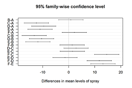
Figure 15-5: Plotting a trend line through the data.

Building a linear model
The lm() function allows you to specify anything from the most simple linear model to complex interaction models. In this section, you build only a simple model to learn how to work with model objects.
To model the mileage in function of the weight of a car, you use the lm() function, like this:
> Model <- lm(mpg ~ wt, data=mtcars)
You supply two arguments:
![]() A formula that describes the model: Here, you model the variable
A formula that describes the model: Here, you model the variable mpg as a function of the variable wt.
![]() A data frame that contains the variables in the formula: Here, you use the data frame
A data frame that contains the variables in the formula: Here, you use the data frame mtcars.
You can specify many complex models with the formula interface when you know your way around. The “Details” section of the Help page ?formula provides all the information you need in great detail.
The resulting object is a list with a very complex structure, but in most cases you don’t need to worry about that. The model object contains a lot of information that’s needed for the calculations of diagnostics and new predictions.
Extracting information from the model
Instead of diving into the model object itself and finding the information somewhere in the list object, you can use some functions that help you to get the necessary information from the model. For example, you can extract a named vector with the coefficients from the model using the coef() function, like this:
> coef.Model <- coef(Model)
> coef.Model
(Intercept) wt
37.285126 -5.344472
These coefficients represent the intercept and the slope of the trend line in Figure 15-5. You can use this to plot the trend line on a scatterplot of the data. You do this in two steps:
1. You plot the scatterplot with the data.
You use the plot() function for that. You discover more about this function in Chapter 16.
2. You use the abline() function to draw the trend line based on the coefficients.
The following code gives you the plot in Figure 15-5:
> plot(mpg ~ wt, data = mtcars)
> abline(a=coef.Model[1], b=coef.Model[2])
The abline() argument a represents the intercept, and b represents the slope of the trend line you want to plot. You plot a vertical line by setting the argument v to the intercept with the x-axis instead. Horizontal lines are plotted by setting the argument v to the intercept with the y-axis.
In Table 15-1, you find an overview of functions to extract information from the model object itself. These functions work with different model objects, including those built by aov() and lm().
Many package authors also provide the same functions for the models built by the functions in their package. So, you can always try to use these extraction functions in combination with other model functions as well.
Table 15-1 Extracting Information from Model Objects
|
Function |
What It Does |
|
|
Returns a vector with the coefficients from the model |
|
|
Returns a matrix with the upper and lower limit of the confidence interval for each coefficient of the model |
|
|
Returns a vector with the fitted values for every observation |
|
|
Returns a vector with the residuals for every observation |
|
|
Returns the variance-covariance matrix for the coefficient |
Evaluating linear models
Naturally, R provides a whole set of different tests and measures to not only look at the model assumptions but also evaluate how well your model fits your data. Again, the overview presented here is far from complete, but it gives you an idea of what’s possible and a starting point to look deeper into the issue.
Summarizing the model
The summary() function immediately returns you the F test for models constructed with aov(). For lm() models, this is slightly different. Take a look at the output:
> Model.summary <- summary(Model)
> Model.summary
Call:
lm(formula = mpg ~ wt, data = mtcars)
Residuals:
Min 1Q Median 3Q Max
-4.5432 -2.3647 -0.1252 1.4096 6.8727
Coefficients:
Estimate Std. Error t value Pr(>|t|)
(Intercept) 37.2851 1.8776 19.858 < 2e-16 ***
wt -5.3445 0.5591 -9.559 1.29e-10 ***
---
Signif. codes: 0 ‘***’ 0.001 ‘**’ 0.01 ‘*’ 0.05 ‘.’ 0.1 ‘ ‘ 1
Residual standard error: 3.046 on 30 degrees of freedom
Multiple R-squared: 0.7528, Adjusted R-squared: 0.7446
F-statistic: 91.38 on 1 and 30 DF, p-value: 1.294e-10
That’s a whole lot of useful information. Here you see the following:
![]() The distribution of the residuals, which gives you a first idea about how well the assumptions of a linear model hold
The distribution of the residuals, which gives you a first idea about how well the assumptions of a linear model hold
![]() The coefficients accompanied by a t-test, telling you in how far every coefficient differs significantly from zero
The coefficients accompanied by a t-test, telling you in how far every coefficient differs significantly from zero
![]() The goodness-of-fit measures R2 and the adjusted R2
The goodness-of-fit measures R2 and the adjusted R2
![]() The F-test that gives you an idea about whether your model explains a significant portion of the variance in your data
The F-test that gives you an idea about whether your model explains a significant portion of the variance in your data
You can use the coef() function to extract a matrix with the estimates, standard errors, and t-value and p-value for the coefficients from the summary object like this:
> coef(Model.summary)
Estimate Std. Error t value Pr(>|t|)
(Intercept) 37.285126 1.877627 19.857575 8.241799e-19
wt -5.344472 0.559101 -9.559044 1.293959e-10
If these terms don’t tell you anything, look them up in a good source about modeling. For an extensive introduction to applying and interpreting linear models correctly, check out Applied Linear Statistical Models, 5th Edition, by Michael Kutner et al (McGraw-Hill/Irwin).
Testing the impact of model terms
To get an analysis of variance table — like the summary() function makes for an ANOVA model — you simply use the anova() function and pass it the lm() model object as an argument, like this:
> Model.anova <- anova(Model)
> Model.anova
Analysis of Variance Table
Response: mpg
Df Sum Sq Mean Sq F value Pr(>F)
wt 1 847.73 847.73 91.375 1.294e-10 ***
Residuals 30 278.32 9.28
---
Signif. codes: 0 ‘***’ 0.001 ‘**’ 0.01 ‘*’ 0.05 ‘.’ 0.1 ‘ ‘ 1
Here, the resulting object is a data frame that allows you to extract any value from that table using the subsetting and indexing tools from Chapter 7. For example, to get the p-value, you can do the following:
> Model.anova[‘wt’,’Pr(>F)’]
[1] 1.293959e-10
You can interpret this value as the probability that adding the variable wt to the model doesn’t make a difference. The low p-value here indicates that the weight of a car (wt) explains a significant portion of the difference in mileage (mpg) between cars. This shouldn’t come as a surprise; a heavier car does, indeed, need more power to drag its own weight around.
The tests done by the anova() function use Type I (sequential) Sum of Squares, which is different from both SAS and SPSS. This also means that the order in which the terms are added to the model has an impact on the test values and the significance.
You can use the anova() function to compare different models as well, and many modeling packages provide that functionality. You find examples of this on most of the related Help pages like ?anova.lm and ?anova.glm.
Predicting new values
Apart from describing relations, models also can be used to predict values for new data. For that, many model systems in R use the same function, conveniently called predict(). Every modeling paradigm in R has a predict function with its own flavor, but in general the basic functionality is the same for all of them.
Getting the values
For example, a car manufacturer has three designs for a new car and wants to know what the predicted mileage is based on the weight of each new design. In order to do this, you first create a data frame with the new values — for example, like this:
> new.cars <- data.frame(wt=c(1.7, 2.4, 3.6))
Always make sure the variable names you use are the same as used in the model. When you do that, you simply call the predict() function with the suited arguments, like this:
> predict(Model, newdata=new.cars)
1 2 3
28.19952 24.45839 18.04503
So, the lightest car has a predicted mileage of 28.2 miles per gallon and the heaviest car has a predicted mileage of 18 miles per gallon, according to this model. Of course, if you use an inadequate model, your predictions can be pretty much off as well.
Having confidence in your predictions
In order to have an idea about the accuracy of the predictions, you can ask for intervals around your prediction. To get a matrix with the prediction and a 95 percent confidence interval around the mean prediction, you set the argument interval to ‘confidence’ like this:
> predict(Model, newdata=new.cars, interval=’confidence’)
fit lwr upr
1 28.19952 26.14755 30.25150
2 24.45839 23.01617 25.90062
3 18.04503 16.86172 19.22834
Now you know that — according to your model — a car with a weight of 2.4 tons has, on average, a mileage between 23 and 25.9 miles per gallon. In the same way, you can ask for a 95 percent prediction interval by setting the argument interval to ‘prediction’:
> predict(Model,newdata=new.cars, interval=’prediction’)
fit lwr upr
1 28.19952 21.64930 34.74975
2 24.45839 18.07287 30.84392
3 18.04503 11.71296 24.37710
This information tells you that 95 percent of the cars with a weight of 2.4 tons have a mileage somewhere between 18.1 and 30.8 miles per gallon — assuming your model is correct, of course.
If you’d rather construct your own confidence interval, you can get the standard errors on your predictions as well by setting the argument se.fit to TRUE. You don’t get a vector or a matrix; instead, you get a list with an element fit that contains the predictions and an element se.fit that contains the standard errors.
..................Content has been hidden....................
You can't read the all page of ebook, please click here login for view all page.