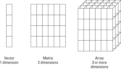
Figure 7-1: A vector, a matrix, and an array.
Chapter 7
Working in More Dimensions
In This Chapter
![]() Creating matrices
Creating matrices
![]() Getting values in and out of a matrix
Getting values in and out of a matrix
![]() Using row and column names in a matrix
Using row and column names in a matrix
![]() Performing matrix calculations
Performing matrix calculations
![]() Working with multidimensional arrays
Working with multidimensional arrays
![]() Putting your data in a data frame
Putting your data in a data frame
![]() Getting data in and out of a data frame
Getting data in and out of a data frame
![]() Working with lists
Working with lists
In the previous chapters, you worked with one-dimensional vectors. The data could be represented by a single row or column in a Microsoft Excel spreadsheet. But often you need more than one dimension. Many calculations in statistics are based on matrices, so you need to be able to represent them and perform matrix calculations. Many datasets contain values of different types for multiple variables and observations, so you need a two-dimensional table to represent this data. In Excel, you would do that in a spreadsheet; in R, you use a specific object called a data frame for the task.
Adding a Second Dimension
In the previous chapters, you constructed vectors to hold series of data in a one-dimensional structure. In addition to vectors, R can represent matrices as an object you work and calculate with. In fact, R really shines when it comes to matrix calculations and operations. In this section, we take a closer look at the magic you can do with them.
Discovering a new dimension
Vectors are closely related to a bigger class of objects, arrays. Arrays have two very important features:
![]() They contain only a single type of value.
They contain only a single type of value.
![]() They have dimensions.
They have dimensions.
The dimensions of an array determine the type of the array. You know already that a vector has only one dimension. An array with two dimensions is a matrix. Anything with more than two dimensions is simply called an array. You find a graphical representation of this in Figure 7-1.
 Technically, a vector has no dimensions at all in R. If you use the functions
 dim(), nrow(), or ncol(), mentioned in the “Looking at the properties” section, later in this chapter, with a vector as argument, R returns NULL as a result.
Creating your first matrix
Creating a matrix is almost as easy as writing the word: You simply use the matrix() function. You do have to give R a little bit more information, though. R needs to know which values you want to put in the matrix and how you want to put them in. The matrix() function has a couple arguments to control this:
![]()
data is a vector of values you want in the matrix.
![]()
ncol takes a single number that tells R how many columns you want.
![]()
nrow takes a single number that tells R how many rows you want.
![]()
byrow takes a logical value that tells R whether you want to fill the matrix row-wise (TRUE) or column-wise (FALSE). Column-wise is the default.
So, the following code results in a matrix with the numbers 1 through 12, in four columns and three rows.
> first.matrix <- matrix(1:12, ncol=4)
> first.matrix
[,1] [,2] [,3] [,4]
[1,] 1 4 7 10
[2,] 2 5 8 11
[3,] 3 6 9 12
 You don’t have to specify both
 ncol and nrow. If you specify one, R will know automatically what the other needs to be.
Alternatively, if you want to fill the matrix row by row, you can do so:
> matrix(1:12, ncol=4, byrow=TRUE)
[,1] [,2] [,3] [,4]
[1,] 1 2 3 4
[2,] 5 6 7 8
[3,] 9 10 11 12
Looking at the properties
 You can look at the structure of an object using the
 str() function. If you do that for your first matrix, you get the following result:
> str(first.matrix)
int [1:3, 1:4] 1 2 3 4 5 6 7 8 9 10 ...
This looks remarkably similar to the output for a vector, with the difference that R gives you both the indices for the rows and for the columns. If you want the number of rows and columns without looking at the structure, you can use the dim() function.
> dim(first.matrix)
[1] 3 4
To get only the number of rows, you use the nrow() function. The ncol() function gives you the number of columns of a matrix.
You can find the total number of values in a matrix exactly the same way as you do with a vector, using the length() function:
> length(first.matrix)
[1] 12
Actually, if you look at the output of the str() function, that matrix looks very much like a vector. That’s because, internally, it’s a vector with a small extra piece of information that tells R the dimensions (see the nearby sidebar, “Playing with attributes”). You can use this property of matrices in calculations, as you’ll see further in this chapter.
Combining vectors into a matrix
In Chapter 4, you created two vectors that contain the number of baskets Granny and Geraldine made in the six games of this basketball season. It would be nicer, though, if the number of baskets for the whole team were contained in one object. With matrices, this becomes possible. You can combine both vectors as two rows of a matrix with the rbind() function, like this:
> baskets.of.Granny <- c(12,4,5,6,9,3)
> baskets.of.Geraldine <- c(5,4,2,4,12,9)
> baskets.team <- rbind(baskets.of.Granny, baskets.of.Geraldine)
If you look at the object baskets.team, you get a nice matrix. As an extra, the rows take the names of the original vectors. You work with these names in the next section.
> baskets.team
[,1] [,2] [,3] [,4] [,5] [,6]
baskets.of.Granny 12 4 5 6 9 3
baskets.of.Geraldine 5 4 2 4 12 9
The cbind() function does something similar. It binds the vectors as columns of a matrix, as in the following example.
> cbind(1:3, 4:6, matrix(7:12, ncol=2))
[,1] [,2] [,3] [,4]
[1,] 1 4 7 10
[2,] 2 5 8 11
[3,] 3 6 9 12
Here you bind together three different nameless objects:
![]() A vector with the values 1 to 3 (
A vector with the values 1 to 3 (1:3)
![]() A vector with the values 4 to 6 (
A vector with the values 4 to 6 (4:6)
![]() A matrix with two columns and three rows, filled column-wise with the values 7 through 12 (
A matrix with two columns and three rows, filled column-wise with the values 7 through 12 (matrix(7:12, ncol=2))
This example shows some other properties of cbind() and rbind() that can be very useful:
![]() The functions work with both vectors and matrices. They also work on other objects, as shown in the “Manipulating Values in a Data Frame” section, later in this chapter.
The functions work with both vectors and matrices. They also work on other objects, as shown in the “Manipulating Values in a Data Frame” section, later in this chapter.
![]() You can give more than two arguments to either function. The vectors and matrices are combined in the order they’re given.
You can give more than two arguments to either function. The vectors and matrices are combined in the order they’re given.
![]() You can combine different types of objects, as long as the dimensions fit. Here you combine vectors and matrices in one function call.
You can combine different types of objects, as long as the dimensions fit. Here you combine vectors and matrices in one function call.
Using the Indices
If you look at the output of the code in the previous section, you’ll probably notice the brackets you used in the previous chapters for accessing values in vectors through the indices. But this time, these indices look a bit different. Where a vector has only one dimension that can be indexed, a matrix has two. The indices for both dimensions are separated by a comma. The index for the row is given before the comma; the index for the column, after it.
Extracting values from a matrix
You can use these indices the same way you use vectors in Chapter 4. You can assign and extract values, use numerical or logical indices, drop values by using a minus sign, and so forth.
Using numeric indices
For example, you can extract the values in the first two rows and the last two columns with the following code:
> first.matrix[1:2, 2:3]
[,1] [,2]
[1,] 4 7
[2,] 5 8
R returns you a matrix again. Pay attention to the indices of this new matrix — they’re not the indices of the original matrix anymore.
R gives you an easy way to extract complete rows and columns from a matrix. You simply don’t specify the other dimension. So, you get the second and third row from your first matrix like this:
> first.matrix[2:3,]
[,1] [,2] [,3] [,4]
[1,] 2 5 8 11
[2,] 3 6 9 12
Dropping values using negative indices
In Chapter 4, you drop values in a vector by using a negative value for the index. This little trick works perfectly well with matrices, too. So, you can get all the values except the second row and third column of first.matrix like this:
> first.matrix[-2,-3]
[,1] [,2] [,3]
[1,] 1 4 10
[2,] 3 6 12
With matrices, a negative index always means: “Drop the complete row or column.” If you want to drop only the element at the second row and the third column, you have to treat the matrix like a vector. So, in this case, you drop the second element in the third column like this:
> nr <- nrow(first.matrix)
> id <- nr*2+2
> first.matrix[-id]
[1] 1 2 3 4 5 6 7 9 10 11 12
This returns a vector, because the 11 remaining elements don’t fit into a matrix anymore. Now what happened here exactly? Remember that matrices are read column-wise. To get the second element in the third column, you need to do the following:
1. Count the number of rows, using nrow(), and store that in a variable — for example nr.
You don’t have to do this, but it makes the code easier to read.
2. Count two columns and then add 2 to get the second element in the third column.
Again store this result in a variable (for example, id).
3. Use the one-dimensional vector extraction [] to drop this value, as shown in Chapter 4.
You can do this in one line, like this:
> first.matrix[-(2 * nrow(first.matrix) + 2)]
[1] 1 2 3 4 5 6 7 9 10 11 12
This is just one example of how you can work with indices while treating a matrix like a vector. It requires a bit of thinking at first, but tricks like these can offer very neat solutions to more complex problems as well, especially if you need your code to run as fast as possible.
Juggling dimensions
As with vectors, you can combine multiple numbers in the indices. If you want to drop the first and third rows of the matrix, you can do so like this:
> first.matrix[-c(1, 3), ]
[1] 2 5 8 11
Wait a minute. . . . There’s only one index. R doesn’t return a matrix here — it returns a vector!
By default, R always tries to simplify the objects to the smallest number of dimensions possible when you use the brackets to extract values from an array. So, if you ask for only one column or row, R will make that a vector by dropping a dimension.
You can force R to keep all dimensions by using the extra argument drop from the indexing function. To get the second row returned as a matrix, you do the following:
> first.matrix[2, , drop=FALSE]
[,1] [,2] [,3] [,4]
[1,] 2 5 8 11
This seems like utter magic, but it’s not that difficult. You have three positions now between the brackets, all separated by commas. The first position is the row index. The second position is the column index. But then what?
Actually, the square brackets work like a function, and the row index and column index are arguments for the square brackets. Now you add an extra argument drop with the value FALSE. As you do with any other function, you separate the arguments by commas. Put all this together, and you have the code shown here.
 The default dropping of dimensions of R can be handy, but it’s famous for being overlooked as well. It can cause serious mishap if you aren’t aware of it. Particularly in code where you take a subset of a matrix, you can easily forget about the case where only one row or column is selected.
Replacing values in a matrix
Replacing values in a matrix is done in a very similar way to replacing values in a vector. To replace the value in the second row and third column of first.matrix with 4, you use the following code.
> first.matrix[3, 2] <- 4
> first.matrix
[,1] [,2] [,3] [,4]
[1,] 1 4 7 10
[2,] 2 5 8 11
[3,] 3 4 9 12
You also can change an entire row or column of values by not specifying the other dimension. Note that values are recycled, so to change the second row to the sequence 1, 3, 1, 3, you can simply do the following:
> first.matrix[2, ] <- c(1,3)
> first.matrix
[,1] [,2] [,3] [,4]
[1,] 1 4 7 10
[2,] 1 3 1 3
[3,] 3 4 9 12
You also can replace a subset of values within the matrix by another matrix. You don’t even have to specify the values as a matrix — a vector will do. Take a look at the result of the following code:
> first.matrix[1:2, 3:4] <- c(8,4,2,1)
> first.matrix
[,1] [,2] [,3] [,4]
[1,] 1 4 8 2
[2,] 1 3 4 1
[3,] 3 4 9 12
Here you change the values in the first two rows and the last two columns to the numbers 8, 4, 2, and 1.
R reads and writes matrices column-wise by default. So, if you put a vector in a matrix or a subset of a matrix, it will be put in column-wise regardless of the method. If you want to do this row-wise, you first have to construct a matrix with the values using the argument byrow=TRUE. Then you use this matrix instead of the original vector to insert the values.
Naming Matrix Rows and Columns
The rbind() function conveniently added the names of the vectors baskets.of.Granny and baskets.of.Geraldine to the rows of the matrix baskets.team in the previous section. You name the values in a vector inChapter 5, and you can do something very similar with rows and columns in a matrix.
For that, you have the functions rownames() and colnames(). Guess which one does what? Both functions work much like the names() function you use when naming vector values. So, let’s check what you can do with these functions.
Changing the row and column names
The matrix baskets.team from the previous section already has some row names. It would be better if the names of the rows would just read ‘Granny’ and ‘Geraldine’. You can easily change these row names like this:
> rownames(baskets.team) <- c(‘Granny’,’Geraldine’)
You can look at the matrix to check if this did what it’s supposed to do, or you can take a look at the row names itself like this:
> rownames(baskets.team)
[1] “Granny” “Geraldine”
The colnames() function works exactly the same. You can, for example, add the number of the game as a column name using the following code:
> colnames(baskets.team) <- c(‘1st’,’2nd’,’3th’,’4th’,’5th’,’6th’)
This gives you the following matrix:
> baskets.team
1st 2nd 3th 4th 5th 6th
Granny 12 4 5 6 9 3
Geraldine 5 4 2 4 12 9
This is almost like you want it, but the third column name contains an annoying writing mistake. No problem there, R allows you to easily correct that mistake. Just as the with names() function, you can use indices to extract or to change a specific row or column name. You can correct the mistake in the column names like this:
> colnames(baskets.team)[3] <- ‘3rd’
If you want to get rid of either column names or row names, the only thing you need to do is set their value to NULL. This also works for vector names, by the way. You can try that out yourself on a copy of the matrix baskets.team like this:
> baskets.copy <- baskets.team
> colnames(baskets.copy) <- NULL
> baskets.copy
[,1] [,2] [,3] [,4] [,5] [,6]
Granny 12 4 5 6 9 3
Geraldine 5 4 2 4 12 9
The row and column names are stored in an attribute called dimnames. To get to the value of that attribute, you can use the dimnames() function to extract or set those values. (See the “Playing with attributes” sidebar, earlier in this chapter, for more information.)
Using names as indices
This naming thing looks remarkably similar to what you can read about naming vectors in Chapter 5. You can use names instead of the index number to select values from a vector. This works for matrices as well, using the row and column names.
Say you want to select the second and the fifth game for both ladies. You can do so using the following code:
> baskets.team[, c(“2nd”,”5th”)]
2nd 5th
Granny 4 9
Geraldine 4 12
Exactly as before, you get all rows if you don’t specify which ones you want. Alternatively, you can extract all the results for Granny like this:
> baskets.team[“Granny”,]
1st 2nd 3rd 4th 5th 6th
12 4 5 6 9 3
That’s the result, indeed, but the row name is gone now. As explained in the “Juggling dimensions” section, earlier in this chapter, R tries to simplify the matrix to a vector, if that’s possible. In this case, a single row is returned so, by default, this is transformed to a vector.
If a one-row matrix is simplified to a vector, the column names are used as names for the values. If a one-column matrix is simplified to a vector, the row names are used as names for the vector.
Calculating with Matrices
Probably the strongest feature of R is its capability to deal with complex matrix operations in an easy and optimized way. Because much of statistics boils down to matrix operations, it’s only natural that R loves to crunch those numbers.
Using standard operations with matrices
When talking about operations on matrices, you can treat either the elements of the matrix or the whole matrix as the value you operate on. That difference is pretty clear when you compare, for example, transposing a matrix and adding a single number (or scalar) to a matrix. When transposing, you work with the whole matrix. When adding a scalar to a matrix, you add that scalar to every element of the matrix.
You add a scalar to a matrix simply by using the addition operator, +, like this:
> first.matrix + 4
[,1] [,2] [,3] [,4]
[1,] 5 8 11 14
[2,] 6 9 12 15
[3,] 7 10 13 16
You can use all other arithmetic operators in exactly the same way to perform an operation on all elements of a matrix.
The difference between operations on matrices and elements becomes less clear if you talk about adding matrices together. In fact, the addition of two matrices is the addition of the responding elements. So, you need to make sure both matrices have the same dimensions.
Let’s look at another example: Say you want to add 1 to the first row, 2 to the second row, and 3 to the third row of the matrix first.matrix. You can do this by constructing a matrix second.matrix that has four columns and three rows and that has 1, 2, and 3 as values in the first, second, and third rows, respectively. The following command does so using the recycling of the first argument by the matrix function (see Chapter 4):
> second.matrix <- matrix(1:3, nrow=3, ncol=4)
With the addition operator, you can add both matrices together, like this:
> first.matrix + second.matrix
[,1] [,2] [,3] [,4]
[1,] 2 5 8 11
[2,] 4 7 10 13
[3,] 6 9 12 15
This is the solution your math teacher would approve of if she asked you to do the matrix addition of the first and second matrix. And even more, if the dimensions of both matrices are not the same, R will complain and refuse to carry out the operation, as shown in the following example:
> first.matrix + second.matrix[,1:3]
Error in first.matrix + second.matrix[, 1:3] : non-conformable arrays
But what would happen if instead of adding a matrix, we added a vector? Take a look at the outcome of the following code:
> first.matrix + 1:3
[,1] [,2] [,3] [,4]
[1,] 2 5 8 11
[2,] 4 7 10 13
[3,] 6 9 12 15
Not only does R not complain about the dimensions, but it recycles the vector over the values of the matrices. In fact, R treats the matrix as a vector in this case by simply ignoring the dimensions. So, in this case, you don’t use matrix addition but simple (vectorized) addition (see Chapter 4).
By default, R fills matrices column-wise. Whenever R reads a matrix, it also reads it column-wise. This has important implications for the work with matrices. If you don’t stay aware of this, R can bite you in the leg nastily.
Calculating row and column summaries
In Chapter 4, you summarize vectors using functions like sum() and prod(). All these functions work on matrices as well, because a matrix is simply a vector with dimensions attached to it. You also can summarize the rows or columns of a matrix using some specialized functions.
In the previous section, you created a matrix baskets.team with the number of baskets that both Granny and Geraldine made in the previous basketball season. To get the total number each woman made during the last six games, you can use the function rowSums() like this:
> rowSums(baskets.team)
Granny Geraldine
39 36
The rowSums() function returns a named vector with the sums of each row.
You can get the means of each row with rowMeans(), and the respective sums and means of each columns with colSums() and colMeans().
Doing matrix arithmetic
Apart from the classical arithmetic operators, R contains a large set of operators and functions to perform a wide set of matrix operations. Many of these operations are used in advanced mathematics, so you may never need them. Some of them can come in pretty handy, though, if you need to flip around data or you want to calculate some statistics yourself.
Transposing a matrix
Flipping around a matrix so the rows become columns and vice versa is very easy in R. The t() function (which stands for transpose) does all the work for you:
> t(first.matrix)
[,1] [,2] [,3]
[1,] 1 2 3
[2,] 4 5 6
[3,] 7 8 9
[4,] 10 11 12
You can try this with a vector, too. As matrices are read and filled column-wise, it shouldn’t come as a surprise that the t() function sees a vector as a one-column matrix. The transpose of a vector is, thus, a one-row matrix:
> t(1:10)
[,1] [,2] [,3] [,4] [,5] [,6] [,7] [,8] [,9] [,10]
[1,] 1 2 3 4 5 6 7 8 9 10
You can tell this is a matrix by the dimensions. This information seems trivial by the way, but imagine you’re selecting only one row from a matrix and transposing it. Unlike what you would expect, you get a row instead of a column:
> t(first.matrix[2,])
[,1] [,2] [,3] [,4]
[1,] 2 5 8 11
Inverting a matrix
Contrary to your intuition, inverting a matrix is not done by raising it to the power of –1. As explained in Chapter 6, R normally applies the arithmetic operators element-wise on the matrix. So, the command first.matrix^(-1) doesn’t give you the inverse of the matrix; instead, it gives you the inverse of the elements. To invert a matrix, you use the solve() function, like this:
> square.matrix <- matrix(c(1,0,3,2,2,4,3,2,1),ncol=3)
> solve(square.matrix)
[,1] [,2] [,3]
[1,] 0.5 -0.8333333 0.1666667
[2,] -0.5 0.6666667 0.1666667
[3,] 0.5 -0.1666667 -0.1666667
Be careful inverting a matrix like this because of the risk of round-off errors. R computes most statistics based on decompositions like the QR decomposition, single-value decomposition, and Cholesky decomposition. You can do that yourself using the functions qr(), svd(), and chol(), respectively. Check the respective Help pages for more information.
Multiplying two matrices
The multiplication operator (*) works element-wise on matrices. To calculate the inner product of two matrices, you use the special operator %*%, like this:
> first.matrix %*% t(second.matrix)
[,1] [,2] [,3]
[1,] 22 44 66
[2,] 26 52 78
[3,] 30 60 90
You have to transpose the second.matrix first; otherwise, both matrices have non-conformable dimensions. Multiplying a matrix with a vector is a bit of a special case; as long as the dimensions fit, R will automatically convert the vector to either a row or a column matrix, whatever is applicable in that case. You can check for yourself in the following example:
> first.matrix %*% 1:4
[,1]
[1,] 70
[2,] 80
[3,] 90
> 1:3 %*% first.matrix
[,1] [,2] [,3] [,4]
[1,] 14 32 50 68
Adding More Dimensions
Both vectors and matrices are special cases of a more general type of object, arrays. All arrays can be seen as a vector with an extra dimension attribute, and the number of dimensions is completely arbitrary. Although arrays with more than two dimensions are not often used in R, it’s good to know of their existence. They can be useful in certain cases, like when you want to represent two-dimensional data in a time series or store multi-way tables in R.
Creating an array
You have two different options for constructing matrices or arrays. Either you use the creator functions matrix() and array(), or you simply change the dimensions using the dim() function.
Using the creator functions
You can create an array easily with the array() function, where you give the data as the first argument and a vector with the sizes of the dimensions as the second argument. The number of dimension sizes in that argument gives you the number of dimensions. For example, you make an array with four columns, three rows, and two “tables” like this:
> my.array <- array(1:24, dim=c(3,4,2))
> my.array
, , 1
[,1] [,2] [,3] [,4]
[1,] 1 4 7 10
[2,] 2 5 8 11
[3,] 3 6 9 12
, , 2
[,1] [,2] [,3] [,4]
[1,] 13 16 19 22
[2,] 14 17 20 23
[3,] 15 18 21 24
This array has three dimensions. Notice that, although the rows are given as the first dimension, the tables are filled column-wise. So, for arrays, R fills the columns, then the rows, and then the rest.
Changing the dimensions of a vector
Alternatively, you could just add the dimensions using the dim() function. This is a little hack that goes a bit faster than using the array() function; it’s especially useful if you have your data already in a vector. (This little trick also works for creating matrices, by the way, because a matrix is nothing more than an array with only two dimensions.)
Say you already have a vector with the numbers 1 through 24, like this:
> my.vector <- 1:24
You can easily convert that vector to an array exactly like my.array simply by assigning the dimensions, like this:
> dim(my.vector) <- c(3,4,2)
If you check how my.vector looks like now, you see there is no difference from the array my.array that you created before.
You can check whether two objects are identical by using the identical() function. To check, for example, whether my.vector and my.array are identical, you simply do the following:
> identical(my.array, my.vector)
[1] TRUE
Using dimensions to extract values
Extracting values from an array with any number of dimensions is completely equivalent to extracting values from a matrix. You separate the dimension indices you want to retrieve with commas, and if necessary you can use the drop argument exactly as you do with matrices. For example, to get the value from the second row and third column of the first table of my.array, you simply do the following:
> my.array[2,3,1]
[1] 8
If you want the third column of the second table as an array, you use the following code:
> my.array[, 3, 2, drop=FALSE]
, , 1
[,1]
[1,] 19
[2,] 20
[3,] 21
If you don’t specify the drop=FALSE argument, R will try to simplify the object as much as possible. This also means that if the result has only two dimensions, R will make it a matrix. The following code returns a matrix that consists of the second row of each table:
> my.array[2, , ]
[,1] [,2]
[1,] 2 14
[2,] 5 17
[3,] 8 20
[4,] 11 23
This reduction doesn’t mean, however, that rows stay rows. In this case, R made the rows columns. This is due to the fact that R first selects the values, and then adds the dimensions necessary to represent the data correctly. In this case R needs two dimensions with four indices (the number of columns) and two indices (the number of tables), respectively. As R fills a matrix column-wise, the original rows now turned into columns.
Combining Different Types of Values in a Data Frame
Prior to this point in the book, you combine values of the same type into either a vector or a matrix. But datasets are, in general, built up from different data types. You can have, for example, the names of your employees, their salaries, and the date they started at your company all in the same dataset. But you can’t combine all this data in one matrix without converting the data to a character data. So, you need a new data structure to keep all this information together in R. That data structure is a data frame.
Creating a data frame from a matrix
Let’s take a look again at the number of baskets scored by Granny and her friend Geraldine. In the “Adding a second dimension” section, earlier in this chapter, you created a matrix baskets.team with the number of baskets for both ladies. It makes sense to make this matrix a data frame with two variables: one containing Granny’s baskets and one containing Geraldine’s baskets.
Using the function as.data.frame
To convert the matrix baskets.team into a data frame, you use the function as.data.frame(), like this:
> baskets.df <- as.data.frame(t(baskets.team))
You don’t have to use the transpose function, t(), to create a data frame, but in our example we want each player to be a separate variable. With data frames, each variable is a column, but in the original matrix, the rows represent the baskets for a single player. So, in order to get the desired result, you first have to transpose the matrix with t() before converting the matrix to a data frame with as.data.frame().
Looking at the structure of a data frame
If you take a look at the object, it looks exactly the same as the transposed matrix t(baskets.team), as shown in the following output:
> baskets.df
Granny Geraldine
1st 12 5
2nd 4 4
3rd 5 2
4th 6 4
5th 9 12
6th 3 9
But there is a very important difference between the two: baskets.df is a data frame. This becomes clear if you take a look at the internal structure of the object, using the str() function:
> str(baskets.df)
‘data.frame’: 6 obs. of 2 variables:
$ Granny : num 12 4 5 6 9 3
$ Geraldine: num 5 4 2 4 12 9
Now this starts looking more like a real dataset. You can see in the output that you have six observations and two variables. The variables are called Granny and Geraldine. It’s important to realize that each variable in itself is a vector; hence, it has one of the types you learn about in Chapters 4, 5, and 6. In this case, the output tells you that both variables are numeric.
Counting values and variables
To know how many observations a data frame has, you can use the nrow() function as you would with a matrix, like this:
> nrow(baskets.df)
[1] 6
Likewise, the ncol() function gives you the number of variables. But you can also use the length() function to get the number of variables for a data frame, like this:
> length(baskets.df)
[1] 2
Creating a data frame from scratch
The conversion from a matrix to a data frame can’t be used to construct a data frame with different types of values. If you combine both numeric and character data in a matrix for example, everything will be converted to character. You can construct a data frame from scratch, though, using the data.frame() function.
Making a data frame from vectors
So, let’s make a little data frame with the names, salaries, and starting dates of a few imaginary co-workers. First, you create three vectors that contain the necessary information like this:
> employee <- c(‘John Doe’,’Peter Gynn’,’Jolie Hope’)
> salary <- c(21000, 23400, 26800)
> startdate <- as.Date(c(‘2010-11-1’,’2008-3-25’,’2007-3-14’))
Now you have three different vectors in your workspace:
![]() A character vector called
A character vector called employee, containing the names
![]() A numeric vector called
A numeric vector called salary, containing the yearly salaries
![]() A date vector called
A date vector called startdate, containing the dates on which the contracts started
Next, you combine the three vectors into a data frame using the following code:
> employ.data <- data.frame(employee, salary, startdate)
The result of this is a data frame, employ.data, with the following structure:
> str(employ.data)
‘data.frame’: 3 obs. of 3 variables:
$ employee : Factor w/ 3 levels “John Doe”,”Jolie Hope”,..: 1 3 2
$ salary : num 21000 23400 26800
$ startdate: Date, format: “2010-11-01” “2008-03-25” ...
To combine a number of vectors into a data frame, you simple add all vectors as arguments to the data.frame() function, separated by commas. R will create a data frame with the variables that are named the same as the vectors used.
Keeping characters as characters
You may have noticed something odd when looking at the structure of employ.data. Whereas the vector employee is a character vector, R made the variable employee in the data frame a factor.
R does this by default, but you have an extra argument to the data.frame() function that can avoid this — namely, the argument stringsAsFactors. In the employ.data example, you can prevent the transformation to a factor of the employee variable by using the following code:
> employ.data <- data.frame(employee, salary, startdate, stringsAsFactors=FALSE)
If you look at the structure of the data frame now, you see that the variable employee is a character vector, as shown in the following output:
> str(employ.data)
‘data.frame’: 3 obs. of 3 variables:
$ employee : chr “John Doe” “Peter Gynn” “Jolie Hope”
$ salary : num 21000 23400 26800
$ startdate: Date, format: “2010-11-01” “2008-03-25” ...
By default, R always transforms character vectors to factors when creating a data frame with character vectors or converting a character matrix to a data frame. This can be a nasty cause of errors in your code if you’re not aware of it. If you make it a habit to always specify the stringsAsFactors argument, you can avoid a lot of frustration.
Naming variables and observations
In the previous section, you select data based on the name of the variables and the observations. These names are similar to the column and row names of a matrix, but there are a few differences as well. We discuss these in the next section.
Working with variable names
Variables in a data frame always need to have a name. To access the variable names, you can again treat a data frame like a matrix and use the function colnames() like this:
> colnames(employ.data)
[1] “employee” “salary” “startdate”
But, in fact, this is taking the long way around. In case of a data frame, the colnames() function lets the hard work be done internally by another function, the names() function. So, to get the variable names, you can just use that function directly like this:
> names(employ.data)
[1] “employee” “salary” “startdate”
Similar to how you do it with matrices, you can use that same function to assign new names to the variables as well. For example, to rename the variable startdate to firstday, you can use the following code:
> names(employ.data)[3] <- ‘firstday’
> names(employ.data)
[1] “employee” “salary” “firstday”
Naming observations
One important difference between a matrix and a data frame is that data frames always have named observations. Whereas the rownames() function returns NULL if you didn’t specify the row names of a matrix, it will always give a result in the case of a data frame.
Check the outcome of the following code:
> rownames(employ.data)
[1] “1” “2” “3”
By default, the row names — or observation names — of a data frame are simply the row numbers in character format. You can’t get rid of them, even if you try to delete them by assigning the NULL value as you can do with matrices.
You shouldn’t try to get rid of them either, because your data frame won’t be displayed correctly any more if you do.
You can, however, change the row names exactly as you do with matrices, simply by assigning the values via the rownames() function, like this:
> rownames(employ.data) <- c(‘Chef’,’BigChef’,’BiggerChef’)
> employ.data
employee salary firstday
Chef John Doe 21000 2010-11-01
BigChef Peter Gynn 23400 2008-03-25
BiggerChef Jolie Hope 26800 2007-03-14
Don’t be fooled, though: Row names can look like another variable, but you can’t access them the way you access the other variables.
Manipulating Values in a Data Frame
Creating a data frame is nice, but data frames would be pretty useless if you couldn’t change the values or add data to them. Luckily, data frames have a very nice feature: When it comes to manipulating the values, almost all tricks you use on matrices can be used on data frames as well. Next to that, you can also use some methods that are designed specifically for data frames. In this next section, we explain these methods for manipulating data frames. For that, we use the data frame baskets.df that you created in the “Creating a data frame from a matrix” section, earlier in this chapter.
Extracting variables, observations, and values
In many cases, you can extract values from a data frame by pretending that it’s a matrix and using the techniques you used in the previous sections as well. But unlike matrices and arrays, data frames are not vectors but lists of vectors. You start with lists in the “Combining different objects in a list” section, later in this chapter. For now, just remember that, although they may look like matrices, data frames are definitely not.
Pretending it’s a matrix
If you want to extract values from a data frame, you can just pretend it’s a matrix and start from there. Both the index numbers and the index names can be used. For example, you can get the number of baskets scored by Geraldine in the third game like this:
> baskets.df[‘3rd’, ‘Geraldine’]
[1] 2
Likewise, you can get all the baskets that Granny scored using the column index, like this:
> baskets.df[, 1]
[1] 12 4 5 6 9 3
Or, if you want this to be a data frame, you can use the argument drop=FALSE exactly as you do with matrices:
> str(baskets.df[, 1, drop=FALSE])
‘data.frame’: 6 obs. of 1 variable:
$ Granny: num 12 4 5 6 9 3
Note that, unlike with matrices, the row names are dropped if you don’t specify the drop=FALSE argument.
Putting your dollar where your data is
As a careful reader, you noticed already that every variable is preceded by a dollar sign ($). R isn’t necessarily pimping your data here — the dollar sign is simply a specific way for accessing variables. To access the variable Granny, you can use the dollar sign like this:
> baskets.df$Granny
[1] 12 4 5 6 9 3
R will return a vector with all the values contained in that variable. Note again that the row names are dropped here.
With this dollar-sign method, you can access only one variable at a time. If you want to access multiple variables at once using their names, you need to use the square brackets, as in the preceding section.
Adding observations to a data frame
As time goes by, new data may appear and needs to be added to the dataset. Just like matrices, data frames can be appended using the rbind() function.
Adding a single observation
Say that Granny and Geraldine played another game with their team, and you want to add the number of baskets they made. The rbind() function lets you do that easily:
> result <- rbind(baskets.df, c(7,4))
> result
Granny Geraldine
1st 12 5
2nd 4 4
3rd 5 2
4th 6 4
5th 9 12
6th 3 9
7 7 4
The data frame result now has an extra observation compared to baskets.df. As explained in the “Combining vectors into a matrix” section, rbind() can take multiple arguments, as long as they’re compatible. In this case, you bind a vector c(7,4) at the bottom of the data frame.
Note that R, by default, sets the row number as the row name for the added rows. You can use the rownames() function to adjust this, or you can do that immediately by specifying the row name between quotes in the rbind() function like this:
> baskets.df <- rbind(baskets.df,’7th’ = c(7,4))
If you check the object baskets.df now, you see the extra observation at the bottom with the correct row name:
> baskets.df
Granny Geraldine
1st 12 5
2nd 4 4
3rd 5 2
4th 6 4
5th 9 12
6th 3 9
7th 7 4
Alternatively, you can use indexing as well, to add an extra observation. You see how in the next section.
Adding a series of new observations using rbind
If you need to add multiple new observations to a data frame, doing it one-by-one is not entirely practical. Luckily, you also can use rbind() to attach a matrix or a data frame with new observations to the original data frame. The matching of the columns is done by name, so you need to make sure that the columns in the matrix or the variables in the data frame with new observations match the variable names in the original data frame.
Let’s add another two game results to the data frame baskets.df. First, you construct a new data frame with the number of baskets Granny and Geraldine scored, like this:
> new.baskets <- data.frame(Granny=c(3,8),Geraldine=c(9,4))
If you use the data.frame() function to construct a new data frame, you can immediately set the variable names by specifying them in the function call, as in the preceding example. That code creates a data frame with the variables Granny and Geraldine where each variable contains the vector given after the equal sign.
To be able to bind the data frame new.baskets to the original baskets.df, you have to make sure that the variable names match exactly, including the case.
Next, you add the optional row names and the necessary column names with the following code:
> rownames(new.baskets) <- c(‘8th’,’9th’)
You also can define the column names yourself as the vector c(‘Granny’,’Geraldine’), but using names(baskets.df) you make sure that the names match perfectly between the data frame baskets.df and the matrix new.baskets.
To add the matrix to the data frame, you simply do the following:
> baskets.df <- rbind(baskets.df, new.baskets)
You can try yourself to do the same thing using a data frame instead of a matrix. In Chapter 13, you use more advanced techniques for combining data from different data frames.
Adding a series of values using indices
You also can use the indices to add a set of new observations at one time. You get exactly the same result if you change all the previous code by this simple line:
> baskets.df[c(‘8th’,’9th’), ] <- matrix(c(3,8,9,4), ncol=2)
With this code, you do the following:
![]() Create a matrix with two columns.
Create a matrix with two columns.
![]() Create a vector with the row names
Create a vector with the row names 8th and 9th.
![]() Use this vector as row indices for the data frame
Use this vector as row indices for the data frame baskets.df.
![]() Assign the values in the matrix to the rows with names
Assign the values in the matrix to the rows with names 8th and 9th. Because these rows don’t exist yet, R will create them automatically.
Actually, you don’t need to construct the matrix first; you can just use a vector instead. Exactly as with matrices, data frames are filled column wise. So, the following code gives you exactly the same result:
> baskets.df[c(‘8th’,’9th’), ] <- c(3,8,9,4)
This process works only for data frames, though. If you try to do the same thing with matrices, you get an error. In the case of matrices, you can only use indices that exist already in the original object.
You have multiple equally valid options for adding observations to a data frame. Which option you choose depends on your personal choice and the situation. If you have a matrix or data frame with extra observations, you can use rbind(). If you have a vector with row names and a set of values, using the indices may be easier.
Adding variables to a data frame
A data frame also can be extended with new variables. You may, for example, get data from another player on Granny’s team. Or you may want to calculate a new variable from the other variables in the dataset, like the total sum of baskets made in each game (see also Chapter 13).
Adding a single variable
There are three main ways of adding a variable. Similar to the case of adding observations, you can use either the cbind() function or the indices. We illustrate both methods later in this section.
You also can use the dollar sign to add an extra variable. Imagine that Granny asked you to add the number of baskets of her friend Gabrielle to the data frame. First, you would create a vector with that data like this:
> baskets.of.Gabrielle <- c(11,5,6,7,3,12,4,5,9)
To create an extra variable named Gabrielle with that data, you simply do the following:
> baskets.df$Gabrielle <- baskets.of.Gabrielle
If you wanted to check whether this worked, but you didn’t want to display the complete data frame, you could use the head() function. This function takes two arguments: the object you want to display and the number of rows you want to see. To see the first four rows of the new data frame, baskets.df, use the following code:
> head(baskets.df, 4)
Granny Geraldine Gabrielle
1st 12 5 11
2nd 4 4 5
3rd 5 2 6
4th 6 4 7
Adding multiple variables using cbind
As we mention earlier, you can pretend your data frame is a matrix and use the cbind() function to do this. Contrary to when you use rbind() on data frames, you don’t even need to worry about the row or column names. Let’s create a new data frame with the goals for Gertrude and Guinevere. You can combine both into a data frame by typing the following code in the editor and running it in the console:
> new.df <- data.frame(
+ Gertrude = c(3,5,2,1,NA,3,1,1,4),
+ Guinevere = c(6,9,7,3,3,6,2,10,6)
+ )
Although the row names of the data frames new.df and baskets.df differ, R will ignore this and just use the row names of the first data frame in the cbind() function, as you can see from the output of the following code:
> head(cbind(baskets.df, new.df), 4)
Granny Geraldine Gabrielle Gertrude Guinevere
1st 12 5 11 3 6
2nd 4 4 5 5 9
3rd 5 2 6 2 7
4th 6 4 7 1 3
When using a data frame or a matrix with column names, R will use those as the names of the variables. If you use cbind() to add a vector to a data frame, R will use the vector’s name as a variable name unless you specify one yourself, as you did with rbind().
If you bind a matrix without column names to the data frame, R will automatically use the column numbers as names. That will cause a bit of trouble though, because plain numbers are invalid object names and, hence, more difficult to use as variable names. In this case, you’d better use the indices.
Whenever you want to use a data frame and don’t want to continuously have to type its name followed by $, you can use the functions with() and within(), as explained in Chapter 13. With the within() function, you also can easily add variables to a data frame.
Combining Different Objects in a List
In the previous sections, you discover how much data frames and matrices are treated alike by many R functions. But contrary to what you would expect, data frames are not a special case of matrices but a special case of lists. A list is a very general and flexible type of object in R. Many statistical functions you use in Chapters 14 and 15 give a list as output. Lists also can be very helpful to group different types of objects, or to carry out operations on a complete set of different objects. You do the latter in Chapter 9.
Creating a list
It shouldn’t come as a surprise that you create a list with the list() function. You can use list() function in two ways: to create an unnamed list or to create a named list. The difference is small; in both cases, think of a list as a big box filled with a set of bags containing all kinds of different stuff. If these bags are labeled instead of numbered, you have a named list.
Creating an unnamed list
Creating an unnamed list is as easy as using the list() function and putting all the objects you want in that list between the (). In the previous sections, you worked with the matrix baskets.team, containing the number of baskets Granny and Geraldine scored this basketball season. If you want to combine this matrix with a character vector indicating which season we’re talking about here, you simply do the following:
> baskets.list <- list(baskets.team, ‘2010-2011’)
If you look now at the object baskets.list, you see the following output:
> baskets.list
[[1]]
1st 2nd 3rd 4th 5th 6th
Granny 12 4 5 6 9 3
Geraldine 5 4 2 4 12 9
[[2]]
[1] “2010-2011”
The object baskets.list contains two elements: the matrix and the season. The numbers between the [[]] indicate the “bag number” of each element.
Creating a named list
In order to create a labeled, or named, list, you simply add the labels before the values between the () of the list() function, like this:
> baskets.nlist <- list(scores=baskets.team, season=’2010-2011’)
This is exactly the same thing you do with data frames in the “Manipulating Values in a Data Frame” section, earlier in this chapter. And that shouldn’t surprise you, because data frames are, in fact, a special kind of named lists.
If you look at the named list baskets.nlist, you see the following output:
> baskets.nlist
$scores
1st 2nd 3rd 4th 5th 6th
Granny 12 4 5 6 9 3
Geraldine 5 4 2 4 12 9
$season
[1] “2010-2011”
Now the [[]] moved out and made a place for the $ followed by the name of the element. In fact, this begins to look a bit like a data frame.
Data frames are nothing but a special type of named lists, so all the tricks in the following sections can be applied to data frames as well. We repeat: All the tricks in the following sections — really, all of them — can be used on data frames as well.
Playing with the names of elements
Just as with data frames, the names of a list are accessed using the names() function, like this:
> names(baskets.nlist)
[1] “scores” “season”
This means that you also can use the names() function to add names to the elements or change the names of the elements in the list in much the same way you do with data frames.
Getting the number of elements
Data frames are lists, so it’s pretty obvious that the number of elements in a list is considered the length of that list. So, to know how many elements you have in baskets.list, you simply do the following:
> length(baskets.list)
[1] 2
Extracting elements from lists
The display of both the unnamed list baskets.list and the named list baskets.nlist show already that the way to access elements in a list differs from the methods you’ve used until now.
That’s not completely true, though. In the case of a named list, you can access the elements using the $, as you do with data frames. For both named and unnamed lists, you can use two other methods to access elements in a list:
![]() Using
Using [[]] gives you the element itself.
![]() Using
Using [] gives you a list with the selected elements.
Using [[]]
If you need only a single element and you want the element itself, you can use [[]], like this:
> baskets.list[[1]]
1st 2nd 3rd 4th 5th 6th
Granny 12 4 5 6 9 3
Geraldine 5 4 2 4 12 9
If you have a named list, you also can use the name of the element as an index, like this:
> baskets.nlist[[‘scores’]]
1st 2nd 3rd 4th 5th 6th
Granny 12 4 5 6 9 3
Geraldine 5 4 2 4 12 9
In each case, you get the element itself returned. Both methods give you the original matrix baskets.team.
You can’t use logical vectors or negative numbers as indices when using [[]]. You can use only a single value — either a (positive) number or an element name.
Using []
You can use [] to extract either a single element or multiple elements from a list, but in this case the outcome is always a list. [] are more flexible than [[]], because you can use all the tricks you also use with vector and matrix indices. [] can work with logical vectors and negative indices as well.
So, if you want all elements of the list baskets.list except for the first one, you can use the following code:
> baskets.list[-1]
[[1]]
[1] “season 2010-2011”
Or if you want all elements of baskets.nlist where the name equals ‘season’, you can use the following code:
> baskets.nlist[names(baskets.nlist)==’season’]
$season
[1] “2010-2011”
Note that, in both cases, the returned value is a list, even if it contains only one element. R simplifies arrays by default, but the same doesn’t count for lists.
Changing the elements in lists
Much like all other objects we cover up to this point, lists aren’t static objects. You can change elements, add elements, and remove elements from them in a pretty straightforward matter.
Changing the value of elements
Assigning a new value to an element in a list is pretty straightforward. You use either the $ or the [[]] to access that element, and simply assign a new value. If you want to replace the scores in the list baskets.nlist with the data frame baskets.df, for example, you can use any of the following options:
> baskets.nlist[[1]] <- baskets.df
> baskets.nlist[[‘scores’]] <- baskets.df
> baskets.nlist$scores <- baskets.df
If you use [], the story is a bit different. You can change elements using [] as well, but you have to assign a list of elements. So, to do the same as the preceding options using [], you need to use following code:
> baskets.nlist[1] <- list(baskets.df)
All these options have exactly the same result, so you may wonder why you would ever use the last option. Simple: Using [] allows you to change more than one element at once. You can change both the season and the scores in baskets.list with the following line of code:
> baskets.list[1:2] <- list(baskets.df, ‘2009-2010’)
This line replaces the first element in baskets.list with the value of baskets.df, and the second element of baskets.list with the character value ‘2009-2010’.
Removing elements
Removing elements is even simpler: Just assign the NULL value to the element. In most cases, the element is simply removed. To remove the first element from baskets.nlist, you can use any of these (and more) options:
> baskets.nlist[[1]] <- NULL
> baskets.nlist$scores <- NULL
> baskets.nlist[‘scores’] <- NULL
Using single brackets, you again have the possibility of deleting more than one element at once. Note that, in this case, you don’t have to create a list with the value NULL first. To the contrary, if you were to do so, you would give the element the value NULL instead of removing it, as shown in the following example:
> baskets.nlist <- list(scores=baskets.df, season=’2010-2011’)
> baskets.nlist[‘scores’] <- list(NULL)
> baskets.nlist
$scores
NULL
$season
[1] “2010-2011”
Adding extra elements using indices
In the section “Adding variables to a data frame,” earlier in this chapter, you use either the $ or indices to add extra variables. Lists work the same way; to add an element called players to the list baskets.nlist, you can use any of the following options:
> baskets.nlist$players <- c(‘Granny’,’Geraldine’)
> baskets.nlist[[‘players’]] <- c(‘Granny’,’Geraldine’)
> baskets.nlist[‘players’] <- list(c(‘Granny’,’Geraldine’))
Likewise, to add the same information as a third element to the list baskets.list, you can use any of the following options:
> baskets.list[[3]] <- c(‘Granny’,’Geraldine’)
> baskets.list[3] <- list(c(‘Granny’,’Geraldine’))
These last options require you to know exactly how many elements a list has before adding an extra element. If baskets.list contained three elements already, you would overwrite that one instead of adding a new one.
Combining lists
If you wanted to add elements to a list, it would be nice if you could do so without having to worry about the indices at all. For that, the only thing you need is a function you use extensively in all the previous chapters, the c() function.
That’s right, the c() function — which is short for concatenate — does a lot more than just creating vectors from a set of values. The c() function can combine different types of objects and, thus, can be used to combine lists into a new list as well.
In order to be able to add the information about the players, you have to create a list first. To make sure you have the same output, you have to rebuild the original baskets.list as well. You can do both using the following code:
> baskets.list <- list(baskets.team,’2010-2011’)
> players <- list(rownames(baskets.team))
Then you can combine this players list with the list goal.list like this:
> c(baskets.list, players)
[[1]]
1st 2nd 3rd 4th 5th 6th
Granny 12 4 5 6 9 3
Geraldine 5 4 2 4 12 9
[[2]]
[1] “2010-2011”
[[3]]
[1] “Granny” “Geraldine”
If any of the lists contains names, these names are preserved in the new object as well.
Reading the output of str() for lists
Many people who start with R get confused by lists in the beginning. There’s really no need for that — there are only two important parts in a list: the elements and the names. And in the case of unnamed lists, you don’t even have to worry about the latter. But if you look at the structure of baskets.list in the following output, you can see why people often shy away from lists.
> str(baskets.list)
List of 2
$ : num [1:2, 1:6] 12 5 4 4 5 2 6 4 9 12 ...
..- attr(*, “dimnames”)=List of 2
.. ..$ : chr [1:2] “Granny” “Geraldine”
.. ..$ : chr [1:6] “1st” “2nd” “3rd” “4th” ...
$ : chr “2010-2011”
This really looks like some obscure code used by the secret intelligence services during World War II. Still, when you know how to read it, it’s pretty easy to read. So let’s split up the output to see what’s going on here:
![]() The first line simply tells you that
The first line simply tells you that baskets.list is a list with two elements.
![]() The second line contains a
The second line contains a $, which indicates the start of the first element. The rest of that line you should be able to read now: It tells you that this first element is a numeric matrix with two rows and six columns (see the previous sections on matrices).
![]() The third line is preceded by
The third line is preceded by .., indicating that this line also belongs to the first element. If you look at the output of str(baskets.team) you see this line and the following two as well. R keeps the row and column names of a matrix in an attribute called dimnames. In the sidebar “Playing with attributes,” earlier in this chapter, you manipulate those yourself. For now, you have to remember only that an attribute is an extra bit of information that can be attached to almost any object in R.
The dimnames attribute is by itself again a list.
![]() The fourth and fifth lines tell you that this list contains two elements: a character vector of length 2 and one of length 6. R uses the
The fourth and fifth lines tell you that this list contains two elements: a character vector of length 2 and one of length 6. R uses the .. only as a placeholder, so you can read from the indentation which lines belong to which element.
![]() Finally, the sixth line starts again with a
Finally, the sixth line starts again with a $ and gives you the structure of the second element — in this case, a character vector with only one value.
If you look at the output of the str(baskets.nlist), you get essentially the same thing. The only difference is that R now puts the name of each element right after the $.
In many cases, looking at the structure of the output from a function can give you a lot of insight into which information is contained in that object. Often, these objects are lists, and the piece of information you’re looking for is buried somewhere in that list.
Seeing the forest through the trees
Working with lists in R is not difficult when you’re used to it, and lists offer many advantages. You can keep related data neatly together, avoiding an overload of different objects in your workspace. You have access to powerful functions to apply a certain algorithm on a whole set of objects at once. Above all, lists allow you to write flexible and efficient code in R.
Yet, many beginning programmers shy away from lists because they’re overwhelmed by the possibilities. R allows you to manipulate lists in many different ways, but often it isn’t clear what the best way to perform a certain task is.
Very likely, you’ll get into trouble at some point by missing important details, but don’t let that scare you. There are a few simple rules that can prevent much of the pain:
![]() If you can name the elements in a list, do so. Working with names always makes life easier, because you don’t have to remember the order of the elements in the list.
If you can name the elements in a list, do so. Working with names always makes life easier, because you don’t have to remember the order of the elements in the list.
![]() If you need to work on a single element, always use either
If you need to work on a single element, always use either [[]] or $.
![]() If you need to select different elements in a list, always use
If you need to select different elements in a list, always use []. Having named elements can definitely help in this case.
![]() If you need a list as a result of a command, always use
If you need a list as a result of a command, always use [].
![]() If the elements in your list have names, use them!
If the elements in your list have names, use them!
![]() If in doubt, consult the Help files.
If in doubt, consult the Help files.
..................Content has been hidden....................
You can't read the all page of ebook, please click here login for view all page.