Chapter 9
Controlling the Logical Flow
In This Chapter
![]() Making choices based on conditions
Making choices based on conditions
![]() Looping over different values
Looping over different values
![]() Applying functions row-wise and column-wise
Applying functions row-wise and column-wise
![]() Applying functions over values, variables, and list elements
Applying functions over values, variables, and list elements
A function can be nothing more than a simple sequence of actions, but these kinds of functions are highly inflexible. Often, you want to make choices and take action dependent on a certain value.
Choices aren’t the only things that can be useful in functions. Loops can prevent you from having to rewrite the same code over and over again. If you want to calculate the summary statistics on different datasets, for example, you can write the code to calculate those statistics and then tell R to carry out that code for all the datasets you had in mind.
R has a very specific mechanism for looping over values that not only is incredibly powerful, but also poses less trouble when you get the hang of it. Instead of using a classic loop structure, you use a function to apply another function on any of the objects discussed in the previous chapters. This way of looping over values is one of the features that distinguishes R from many other programming languages.
In this chapter, we cover the R tools to create loops and make decisions.
Note: If a piece of code is not preceded by a prompt (>), it represents an example function that you can copy to your editor and then send to the console (as explained in Chapter 2). All code you normally type directly at the command line is preceded by a prompt.
Making Choices with if Statements
Defining a choice in your code is pretty simple: If this condition is true, then carry out a certain task. Many programming languages let you do that with exactly those words: if . . . then. R makes it even easier: You can drop the word then and specify your choice in an if statement.
 An
An if statement in R consists of three elements:
![]() The keyword
The keyword if
![]() A single logical value between parentheses (or an expression that leads to a single logical value)
A single logical value between parentheses (or an expression that leads to a single logical value)
![]() A block of code between braces that has to be executed when the logical value is
A block of code between braces that has to be executed when the logical value is TRUE
To show you how easy this is, let’s write a very small function, priceCalculator(), that calculates the price you charge to a customer based on the hours of work you did for that customer. The function should take the number of hours (hours) and the price per hour (pph) as input. The priceCalculator() function could be something like this:
priceCalculator <- function(hours, pph=40){
net.price <- hours * pph
round(net.price)
}
Here’s what this code does:
![]() With the
With the function keyword, you define the function.
![]() Everything between the braces is the body of the function (see Chapter 8).
Everything between the braces is the body of the function (see Chapter 8).
![]() Between the parentheses, you specify the arguments
Between the parentheses, you specify the arguments hours (without a default value) and pph (with a default value of $40 per hour).
![]() You calculate the net price by multiplying
You calculate the net price by multiplying hours by pph.
![]() The outcome of the last statement in the body of your function is the returned value. In this case, this is the total price rounded to the dollar.
The outcome of the last statement in the body of your function is the returned value. In this case, this is the total price rounded to the dollar.
You could drop the argument pph and just multiply hours by 40. But that would mean that if, for example, your colleague uses a different hourly rate, he would have to change the value in the body of the function in order to be able to use it. It’s good coding practice to use arguments with default values for any value that can change. Doing so makes a function more flexible and usable.
Now imagine you have some big clients that give you a lot of work. To keep them happy, you decide to give them a reduction of 10 percent on the price per hour for orders that involve more than 100 hours of work. So, if the number of hours worked is larger than 100, you calculate the new price by multiplying the price by 0.9. You can write that almost literally in your code like this:
priceCalculator <- function(hours, pph=40){
net.price <- hours * pph
if(hours > 100) {
net.price <- net.price * 0.9
}
round(net.price)
}
Copy this code in a script file, and send it to the console to make it available for use. If you try out this function, you can see that the reduction is given only when the number of hours is larger than 100:
> priceCalculator(hours = 55)
[1] 2200
> priceCalculator(hours = 110)
[1] 3960
 An
An if statement in R consists of three elements: the keyword if, a single logical value between parentheses, and a block of code between braces that has to be executed when the logical value is TRUE. If you look at the if statement in the previous function, you find these three elements. Between the parentheses, you find an expression (hours > 100) that evaluates to a single logical value. Between the braces stands one line of code that reduces the net price by 10 percent when the line is carried out.
This construct is the most general way you can specify an if statement. But if you have only one short line of code in the code block, you don’t have to put braces around it. You can change the complete if statement in the function with the following line:
if(hours > 100) net.price <- net.price * 0.9
The usual way of getting help on a function named, for example, fun.name (?fun.name) does not work for if. To access the built-in help for if, you have to quote the function name. You can use single quotes, double quotes, or backticks. Each of the following statements takes you to the Help page for if:
?’if’
?”if”
?`if`
Doing Something Else with an if...else Statement
In some cases, you need your function to do something if a condition is true and something else if it is not. You could do this with two if statements, but there’s an easier way in R: an if...else statement. An if…else statement contains the same elements as an if statement (see the preceding section), and then some extra:
![]() The keyword
The keyword else, placed after the first code block
![]() A second block of code, contained within braces, that has to be carried out if and only if the result of the condition in the
A second block of code, contained within braces, that has to be carried out if and only if the result of the condition in the if() statement is FALSE
In some countries, the amount of value added tax (VAT) that has to be paid on certain services depends on whether the client is a public or private organization. Imagine that public organizations have to pay only 6 percent VAT and private organizations have to pay 12 percent VAT. You can add an extra argument public to the priceCalculator() function and adopt it as follows to add the correct amount of VAT:
priceCalculator <- function(hours, pph=40, public=TRUE){
net.price <- hours * pph
if(hours > 100) net.price <- net.price * 0.9
if(public) {
tot.price <- net.price * 1.06
} else {
tot.price <- net.price * 1.12
}
round(tot.price)
}
If you send this code to the console, you can test the function. For example, if you worked for 25 hours, the following code gives you the different amounts you charge for public and private organizations, respectively:
> priceCalculator(25,public=TRUE)
[1] 1060
> priceCalculator(25,public=FALSE)
[1] 1120
This works well, but how does it work?
If you look at the if...else statement in the previous function, you find these elements. If the value of the argument public is TRUE, the total price is calculated as 1.06 times the net price. Otherwise, the total price is 1.12 times the net price.
The if statement needs a logical value between the parentheses. Any expression you put between the parentheses is evaluated before it’s passed on to the if statement. So, if you work with a logical value directly, you don’t have to specify an expression at all. Using, for example, if(public == TRUE) is about as redundant as asking if white snow is white. It would work, but it’s bad coding practice.
Also, in the case of an if...else statement you can drop the braces if both code blocks exist of only a single line of code. So, you could just forget about the braces and squeeze the whole if...else statement on a single line. Or you could even write it like this:
if(public) tot.price <- net.price * 1.06 else
tot.price <- net.price * 1.12
Putting the else statement at the end of a line and not the beginning of the next one is a good idea. In general, R reads multiple lines as a single line as long as it’s absolutely clear that the command isn’t finished yet (see Chapter 3). If you put else at the beginning of the second line, R considers the first line finished and complains. You can put else at the beginning of a next line only if you do so within a function and you source the complete file at once to R.
But you can still make this shorter. The if statement works like a function and, hence, it also returns a value. As a result, you can assign that value to an object or use it in calculations. So, instead of recalculating net.price and assigning the result to tot.price within the code blocks, you can use the if...else statement like this:
tot.price <- net.price * if(public) 1.06 else 1.12
R will first evaluate the if...else statement, and multiply the outcome by net.price. The result of this is then assigned to tot.price. This differs not one iota from the result of the five lines of code we used for the original if...else statement. R allows programmers to be incredibly lazy, er, economical here.
Vectorizing Choices
As we discuss in Chapter 4, vectorization is one of the defining attributes of the R language. R wouldn’t be R if it didn’t have some kind of vectorized version of an if...else statement. If you wonder why on earth you would need such a thing, take a look at the problem discussed in this section.
Looking at the problem
The priceCalculator() function still isn’t very economical to use. If you have 100 clients, you’ll have to calculate the price for every client separately. Check for yourself what happens if you add, for example, three different amounts of hours as an argument:
> priceCalculator(c(25,110))
[1] 1060 4664
Warning message:
In if (hours > 100) net.price <- net.price * 0.9 :
the condition has length > 1 and only the first element will be used
Not only does R warn you that something fishy is going on, but the result you get is plain wrong. Instead of $4,664, the second client should be charged only $4,198:
> priceCalculator(110)
[1] 4198
What happened? The warning message should give you a fair idea about what went on. An if statement can deal only with a single value, but the expression hours > 100 returns two values, as shown by the following code:
> c(25, 110) > 100
[1] FALSE TRUE
Choosing based on a logical vector
The solution you’re looking for is the ifelse() function, which is a vectorized way of choosing values from two vectors. This remarkable function takes three arguments:
![]() A test vector with logical values
A test vector with logical values
![]() A vector with values that should be returned if the corresponding value in the test vector is
A vector with values that should be returned if the corresponding value in the test vector is TRUE
![]() A vector with values that should be returned if the corresponding value in the test vector is
A vector with values that should be returned if the corresponding value in the test vector is FALSE
Understanding how it works
Take a look at the following trivial example:
> ifelse(c(1,3) < 2.5 , 1:2 , 3:4)
[1] 1 4
To understand how it works, run over the steps the function takes:
1. The conditional expression c(1,3) < 2.5 is evaluated to a logical vector.
2. The first value of this vector is TRUE, because 1 is smaller than 2.5. So, the first value of the result is the first value of the second argument, which is 1.
3. The next value is FALSE, because 3 is larger than 2.5. Hence, ifelse() takes the second value of the third argument (which is 4) as the second value of the result.
4. A vector with the selected values is returned as the result.
Trying it out
To see how this works in the example of the priceCalculator() function, try the function out at the command line in the console. Say you have two clients and you worked 25 and 110 hours for them, respectively. You can calculate the net price with the following code:
> my.hours <- c(25,110)
> my.hours * 40 * ifelse(my.hours > 100, 0.9, 1)
[1] 1000 3960
Didn’t you just read that the second and third arguments should be a vector? Yes, but the ifelse() function can recycle its arguments. And that’s exactly what it does here. In the preceding ifelse() function call, you translate the logical vector created by the expression my.hours > 100 into a vector containing the numbers 0.9 and 1 in lieu of TRUE and FALSE, respectively.
Adapting the function
Of course, you need to adapt the priceCalculator() function in such a way that you also can input a vector with values for the argument public. Otherwise, you wouldn’t be able to calculate the prices for a mixture of public and private clients. The final function looks like this:
priceCalculator <- function(hours,pph=40,public){
net.price <- hours * pph
net.price <- net.price * ifelse(hours > 100 , 0.9, 1)
tot.price <- net.price * ifelse(public, 1.06, 1.12)
round(price)
}
Next, create a little data frame to test the function. For example:
> clients <- data.frame(
+ hours = c(25, 110, 125, 40),
+ public = c(TRUE,TRUE,FALSE,FALSE)
+)
You can use this data frame now as arguments for the priceCalculator() function, like this:
> with(clients, priceCalculator(hours, public = public))
[1] 1060 4198 5040 1792
There you go. Problem solved!
Making Multiple Choices
The if and if...else statements you use in the previous section leave you with exactly two options, but life is seldom as simple as that. Imagine you have some clients abroad.
Let’s assume that any client abroad doesn’t need to pay VAT for the sake of the example. This leaves you now with three different VAT rates: 12 percent for private clients, 6 percent for public clients, and none for foreign clients.
Chaining if...else statements
The most intuitive way to solve this problem is just to chain the choices. If a client is living abroad, don’t charge any VAT. Otherwise, check whether the client is public or private and apply the relevant VAT rate.
If you define an argument client for your function that can take the values ‘abroad’, ‘public’, and ‘private’, you could code the previous algorithm like this:
if(client==’private’){
tot.price <- net.price * 1.12 # 12% VAT
} else {
if(client==’public’){
tot.price <- net.price * 1.06 # 6% VAT
} else {
tot.price <- net.price * 1 # 0% VAT
}
}
With this code, you nest the second if...else statement in the first if...else statement. That’s perfectly acceptable and it will work, but imagine what you would have to do if you had four or even more possibilities. Nesting a statement in a statement in a statement in a statement quickly creates one huge curly mess.
Luckily, R allows you to write all that code a bit more clearly. You can chain the if...else statements as follows:
if(client==’private’){
tot.price <- net.price * 1.12
} else if(client==’public’){
tot.price <- net.price * 1.06
} else {
tot.price <- net.price
}
In this example, the chaining makes a difference of only two braces, but when you have more possibilities, it really makes the difference between readable code and sleepless nights. Note, also, that you don’t have to test whether the argument client is equal to ‘abroad’ (although it wouldn’t be wrong to do that). You just assume that if client doesn’t have any of the two other values, it has to be ‘abroad’.
Chained if...else statements work on a single value at a time. You can’t use these chained if...else statements in a vectorized way. For that, you can nest multiple ifelse statements, like this:
VAT <- ifelse(client==’private’, 1.12,
ifelse(client == ‘public’, 1.06, 1)
)
tot.price <- net.price * VAT
This piece of code can become quite confusing if you have more than three choices, though. The solution to this is to switch.
Switching between possibilities
The nested if...else statement is especially useful if you have complete code blocks that have to be carried out when a condition is met. But if you need to select values based only on a condition, there’s a better option: Use the switch() function.
Making choices with switch
In the previous example, you wanted to adjust the VAT rate depending on whether the client is a public one, is a private one, or lives abroad. You have a list of three possible choices, and for each choice you have a specific VAT rate. You can use the switch() function like this:
VAT <- switch(client, private=1.12, public=1.06, abroad=1)
You construct a switch() call as follows:
1. Give a single value as the first argument (in this case, the value of client).
Note that switch() isn’t vectorized, so it can’t deal with vectors as a first argument.
2. After the first argument, you give a list of choices with the respected values.
Note that you don’t have to put quotation marks around the choices.
Remember that switch() doesn’t work in a vectorized way. You can distinguish the choices more easily, however, so the code becomes more readable.
 In fact, the first argument doesn’t have to be a value; it can be some expression that evaluates to either a character vector or a number. In case you work with numbers, you don’t even have to use
 choice=value in the function call. If you have integers, switch() will return the option in that position. In the statement switch(2,’some value’, ‘something else’, ‘some more’), the result is ‘something else’. You can find more information and examples on the Help page ?switch.
Using default values in switch
You don’t have to specify all options in a switch() call. If you want to have a certain result in case the matched value is not among the specified options, put that result as the last option, without any choice before it. So, the following line of code does exactly the same thing as the nested ifelse call from “Chaining if...else statements” section, earlier in this chapter:
VAT <- switch(client, private=1.12, public=1.06, 1)
You can easily test this out in the console by creating an object called client with a certain value and then running the switch() call, as in the following example:
> client <- ‘other’
> switch(client, private=1.12, public=1.06, 1)
[1] 1
You can give client different values to see how switch() works.
Looping Through Values
In the previous section, you use a couple different methods to make choices. Many of these methods aren’t vectorized, so you can use only a single value to base your choice on. You could, of course, apply that code on each value you have by hand, but it makes far more sense to automate this task.
Constructing a for loop
As in many other programming languages, you repeat an action for every value in a vector by using a for loop. You construct a for loop in R as follows:
for(i in values){
... do something ...
}
This for loop consists of the following parts:
![]() The keyword
The keyword for, followed by parentheses.
![]() An identifier between the parentheses. In this example, we use
An identifier between the parentheses. In this example, we use i, but that can be any object name you like.
![]() The keyword
The keyword in, which follows the identifier.
![]() A vector with values to loop over. In this example code, we use the object
A vector with values to loop over. In this example code, we use the object values, but that again can be any vector you have available.
![]() A code block between braces that has to be carried out for every value in the object
A code block between braces that has to be carried out for every value in the object values.
In the code block, you can use the identifier. Each time R loops through the code, R assigns the next value in the vector with values to the identifier.
Calculating values in a for loop
Let’s take another look at the priceCalculator() function (refer to the “Making Multiple Choices” section, earlier in this chapter). Earlier, we show you a few possibilities to adapt this function so you can apply a different VAT rate for public, private, and foreign clients. You can’t use any of these options in a vectorized way, but you can use a for loop so the function can calculate the price for multiple clients at once.
Using the values of the vector
Adapt the priceCalculator() function as follows:
priceCalculator <- function(hours, pph=40, client){
net.price <- hours * pph *
ifelse(hours > 100, 0.9, 1)
VAT <- numeric(0)
for(i in client){
VAT <- c(VAT,switch(i, private=1.12, public=1.06, 1))
}
tot.price <- net.price * VAT
round(tot.price)
}
The first and the last part of the function haven’t changed, but in the middle section, you do the following:
1. Create a numeric vector with length 0 and call it VAT.
2. For every value in the vector client, apply switch() to select the correct amount of VAT to be paid.
3. In each round through the loop, add the outcome of switch() at the end of the vector VAT.
The result is a vector VAT that contains, for each client, the correct VAT that needs to be applied. You can test this by adding, for example, a variable type to the data frame clients you created in the previous section like this:
> clients$type <- c(‘public’,’abroad’,’private’,’abroad’)
> priceCalculator(clients$hours, client=clients$type)
[1] 1060 3960 5040 1600
Using loops and indices
The function from the previous section works, but you can write more efficient code if you loop not over the values but over the indices. To do so, you replace the middle section in the function with the following code:
nclient <- length(client)
VAT <- numeric(nclient)
for(i in seq_along(client)){
VAT[i] <- switch(client[i], private=1.12, public=1.06, 1))
}
This code acts very similar to the previous one, but there are a few differences:
![]() You assign the length of the vector
You assign the length of the vector client to the variable nclient.
![]() Then you make a numeric vector
Then you make a numeric vector VAT that is exactly as long as the vector client. This is called pre-allocation of a vector.
![]() Then you loop over indices of client instead of the vector itself by using the function
Then you loop over indices of client instead of the vector itself by using the function seq_along(). In the first pass through the loop, the first value in VAT is set to be the result of switch() applied to the first value in client. In the second pass, the second value of VAT is the result of switch() applied to the second value in client and so on.
You may be tempted to replace seq_along(client) with the vector 1:nclient, but that would be a bad idea. If the vector client has a length of 0, seq_along(client) creates an empty vector and the code in the loop never executes. If you use 1:nclient, R creates a vector c(1,0) and loop over those two values, giving you a completely wrong result.
Doing more with loops — and when not to do so
R contains some of the mechanisms used in other programming languages to manipulate loops:
![]() The keyword
The keyword next, to skip to the next iteration of a loop without running the remaining code in the code block
![]() The keyword
The keyword break, to break out of a loop at any given point
![]() The keyword
The keyword while, to construct a loop that continues as long as a certain condition is TRUE.
You find more information on the use of these keywords on the Help page ?Control.
Although you can technically use all three options, they’re not often used. Many programmers consider the use of break and next to be bad coding practice in any language.
For while, the situation is a bit more complex. A while loop is useful only in very specific cases, like when you generate artificial data that has to meet certain conditions or when you write your own optimization algorithms. But in many cases the built-in optimization functions like optim(), optimize(), and nlm() work faster than a while loop — and often more stable. These functions require a bit of study before you can apply them, but studying the Help pages ?optim, ?optimize, and ?nlm, as well as related pages, can really pay off.
Every time you lengthen an object in R, R has to copy the whole object and move it to a new place in the memory. This has two effects: First, it slows down your code, because all the copying takes time. Second, as R continuously moves things around in memory, this memory gets split up in a lot of small spaces. This is called fragmentation, and it makes the communication between R and the memory less smooth. You can avoid this fragmentation by pre-allocating memory as in the previous example.
Looping without Loops: Meeting the Apply Family
Using for loops has some important side effects that some people would call serious drawbacks. For one, the objects you create in the for loop stay in the workspace afterward. Objects you change in the for loop are changed in the workspace. This may be exactly what you’re trying to do, but more often than not, this is an unwanted side effect of the way for loops are implemented in R.
Take a look at the following trivial example:
> songline <- ‘Get out of my dreams...’
> for(songline in 1:5) print(‘...Get into my car!’)
Contrary to what you may expect, after running this code, the value of songline is not the string ‘Get out of my dreams...’, but the number 5, as shown in the output below:
> songline
[1] 5
Although you never explicitly changed the value of songline anywhere in the code, R does so implicitly when carrying out the for loop. Every iteration, R reassigns the next value from the vector to songline . . . in the workspace! By choosing the names of the variables and the identifier wisely, you can avoid running into this kind of trouble. But when writing large scripts, you need to do some serious bookkeeping for the names, and making mistakes becomes all too easy.
To be completely correct, using a for loop has an effect on the environment you work in at that moment. If you just use the for loop in scripts that you run in the console, the effects will take place in the workspace. If you use a for loop in the body of the function, the effects will take place within the environment of that function. For more information, see Chapter 8.
Here’s the good news: R has another looping system that’s very powerful, that’s at least as fast as for loops (and sometimes much faster), and — most important of all — that doesn’t have the side effects of a for loop. Actually, this system consists of a complete family of related functions, known as the apply family. This family contains seven functions, all ending with apply.
Looking at the family features
Before you start using any of the functions in the apply family, here are the most important properties of these functions:
![]() Every one of the apply functions takes at least two arguments: an object and another function. You pass the function as an argument (see Chapter 8).
Every one of the apply functions takes at least two arguments: an object and another function. You pass the function as an argument (see Chapter 8).
![]() None of these apply functions has side effects. This is the main reason to use them, so we can’t stress it enough: If you can use any apply function instead of a
None of these apply functions has side effects. This is the main reason to use them, so we can’t stress it enough: If you can use any apply function instead of a for loop, use the apply solution. Be aware, though, that possible side effects of the applied function are not taken care of by the apply family.
![]() Every apply function can pass on arguments to the function that is given as an argument. It does that using the
Every apply function can pass on arguments to the function that is given as an argument. It does that using the dots argument (see Chapter 8).
![]() Every function of the apply family always returns a result. Using the apply family makes sense only if you need that result. If you want to print messages to the console with
Every function of the apply family always returns a result. Using the apply family makes sense only if you need that result. If you want to print messages to the console with print() or cat() for example, there’s no point in using the apply family for that.
Meeting three of the members
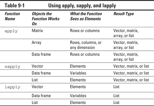
Say hello to apply(), sapply(), and lapply(), the most used members of the apply family. Every one of these functions applies another function to all elements in an object. What those elements are depends on the object and the function. Table 9-1 provides an overview of the objects that each of these three functions works on, what each function sees as an element, and which objects each function can return. We explain how to use these functions in the remainder of this chapter.
Applying functions on rows and columns
In Chapter 7, you calculate the sum of a matrix with the rowSums() function. You can do the same for means with the rowMeans() function, and you have the related functions colSums() and colMeans() to calculate the sum and the mean for each column. But R doesn’t have similar functions for every operation you want to carry out. Luckily, you can use the apply() function to apply a function over every row or column of a matrix or data frame.
Counting birds
Imagine you counted the birds in your backyard on three different days and stored the counts in a matrix like this:
> counts <- matrix(c(3,2,4,6,5,1,8,6,1), ncol=3)
> colnames(counts) <- c(‘sparrow’,’dove’,’crow’)
> counts
sparrow dove crow
[1,] 3 6 8
[2,] 2 5 6
[3,] 4 1 1
Each column represents a different species, and each row represents a different day. Now you want to know the maximum count per species on any given day. You could construct a for loop to do so, but using apply(), you do this in only one line of code:
> apply(counts, 2, max)
sparrow dove crow
4 6 8
The apply() function returns a vector with the maximum for each column and conveniently uses the column names as names for this vector as well. If R doesn’t find names for the dimension over which apply() runs, it returns an unnamed object instead.
Let’s take a look at how this apply() function works. In the previous lines of code, you used three arguments:
![]() The object on which the function has to be applied: In this case, it’s the matrix
The object on which the function has to be applied: In this case, it’s the matrix counts.
![]() The dimension or index over which the function has to be applied: The number
The dimension or index over which the function has to be applied: The number 1 means row-wise, and the number 2 means column-wise. Here, we apply the function over the columns. In the case of more-dimensional arrays, this index can be larger than 2.
![]() The name of the function that has to be applied: You can use quotation marks around the function name, but you don’t have to. Here, we apply the function
The name of the function that has to be applied: You can use quotation marks around the function name, but you don’t have to. Here, we apply the function max. Note that there are no parentheses needed after the function name.
The apply() function splits up the matrix (or data frame) in rows (or columns). Remember that if you select a single row or column, R will, by default, simplify that to a vector. The apply() function then uses these vectors one by one as an argument to the function you specified. So, the applied function needs to be able to deal with vectors.
Adding extra arguments
Let’s go back to our example from the preceding section: Imagine you didn’t look for doves the second day. This means that, for that day, you don’t have any data, so you have to set that value to NA like this:
> counts[2, 2] <- NA
If you apply the max function on the columns of this matrix, you get the following result:
> apply(counts,2,max)
sparrow dove crow
4 NA 8
That’s not what you want. In order to deal with the missing values, you need to pass the argument na.rm to the max function in the apply() call (see Chapter 4). Luckily, this is easily done in R. You just have to add all extra arguments to the function as extra arguments of the apply() call, like this:
> apply(counts, 2, max, na.rm=TRUE)
sparrow dove crow
4 6 8
You can pass any arguments you want to the function in the apply() call by just adding them between the parentheses after the first three arguments.
Applying functions to listlike objects
The apply() function works on anything that has dimensions, but what if you don’t have dimensions (for example, when you have a list or a vector)? For that, you have two related functions from the apply family at your disposal: sapply() and lapply(). The l in lapply stands for list, and the s in sapply stands for simplify. The two functions work basically the same — the only difference is that lapply() always returns a list with the result, whereas sapply() tries to simplify the final object if possible.
Applying a function to a vector
As you can see in Table 9-1, both sapply() and lapply() consider every value in the vector to be an element on which they can apply a function. Many functions in R work in a vectorized way, so there’s often no need to use this.
Using switch on vectors
The switch() function, however, doesn’t work in a vectorized way. Consider the following basic example:
> sapply(c(‘a’,’b’), switch, a=’Hello’, b=’Goodbye’)
a b
“Hello” “Goodbye”
The sapply() call works very similar to the apply() call from the previous section, although you don’t have an argument that specifies the index. Here’s a recap:
![]() The first argument is the vector on which values you want to apply the function — in this case, the vector
The first argument is the vector on which values you want to apply the function — in this case, the vector c(‘a’, ‘b’).
![]() The second argument is the name of the function — in this case,
The second argument is the name of the function — in this case, switch.
![]() All other arguments are simply the arguments you pass to the
All other arguments are simply the arguments you pass to the switch function.
The sapply() function now takes first the value ‘a’ and then the value ‘b’ as the first argument to switch(), using the arguments a=’Hello’ and b=’Goodbye’ each time as the other arguments. It combines both results into a vector and uses the values of c(‘a’, ‘b’) as names for the resulting vector.
The sapply() function has an argument USE.NAMES that you can set to FALSE if you don’t want sapply() to use character values as names for the result. For details about this argument, see the Help page ?sapply.
Replacing a complete for loop with a single statement
In the “Calculating values in a for loop” section, earlier in this chapter, you use a for loop to apply the switch() function on all values passed through the argument client. Although that trick works nicely, you can replace the pre-allocation and the loop with one simple statement, like this:
priceCalculator <- function(hours, pph=40, client){
net.price <- hours * pph * ifelse(hours > 100, 0.9, 1)
VAT <- sapply(client, switch, private=1.12, public=1.06, 1)
tot.price <- net.price * VAT
round(tot.price)
}
Applying a function to a data frame
You also can use sapply() on lists and data frames. In this case, sapply() applies the specified function on every element in that list. Because data frames are lists as well, everything in this section applies to both lists and data frames.
Imagine that you want to know which type of variables you have in your data frame clients. For a vector, you can use the class() function to find out the type. In order to know this for all variables of the data frame at once, you simply apply the class() function to every variable by using sapply() like this:
> sapply(clients,class)
hours public type
“numeric” “logical” “character”
R returns a named vector that gives you the types of every variable, and it uses the names of the variables as names for the vector. In case you use a named list, R uses the names of the list elements as names for the vector.
Simplifying results (or not) with sapply
The sapply() function doesn’t always return a vector. In fact, the standard output of sapply is a list, but that list gets simplified to either a matrix or a vector if possible.
![]() If the result of the applied function on every element of the list or vector is a single number,
If the result of the applied function on every element of the list or vector is a single number, sapply() simplifies the result to a vector.
![]() If the result of the applied function on every element of the list or vector is a vector with exactly the same length,
If the result of the applied function on every element of the list or vector is a vector with exactly the same length, sapply() simplifies the result to a matrix.
![]() In all other cases,
In all other cases, sapply() returns a (named) list with the results.
Say you want to know the unique values of every variable in the data frame clients. To get all unique values in a vector, you use the unique() function. You can get the result you want by applying that function to the data frame clients like this:
> sapply(clients, unique)
$hours
[1] 25 110 125 40
$public
[1] TRUE FALSE
$type
[1] “public” “abroad” “private”
In the variable hours, you find four unique values; in the variable public, only two; and in the variable type, three. Because the lengths of the result differ for every variable, sapply() can’t simplify the result, so it returns a named list.
Getting lists using lapply
The lapply() function works exactly the same as the sapply() function, with one important difference: It always returns a list. This trait can be beneficial if you’re not sure what the outcome of sapply() will be.
Say you want to know the unique values of only a subset of the data frame clients. You can get the unique values in the first and third rows of the data frame like this:
> sapply(clients[c(1,3), ], unique)
hours public type
[1,] “25” “TRUE” “public”
[2,] “125” “FALSE” “private”
But because every variable now has two unique values, sapply() simplifies the result to a matrix. If you counted on the result to be a list in the following code, you would get errors. If you used lapply(), on the other hand, you would also get a list in this case, as shown in the following output:
> lapply(clients[c(1,3), ], unique)
$hours
[1] 25 125
$public
[1] TRUE FALSE
$type
[1] “public” “private”
Actually, the sapply() function has an extra argument, simplify, that you can set to FALSE if you don’t want a simplified list. If you set both the arguments simplify and USE.NAMES to FALSE, sapply() and lapply() return exactly the same result. For details on the difference between the two functions, look at the Help file ?sapply.