Chapter 8

Putting the Fun in Functions

In This Chapter

Automating your work with functions

Playing with arguments

Finding objects within the functions

Working with methods

Automating your work is probably the number-one reason why you use a programming language. For that, you can get pretty far with the built-in functions of R in combination with scripts, but scripts aren’t very flexible when dealing with variable input. Luckily, R allows you to write your own custom functions (for example, to automate the cleaning of your data, to apply a series of analyses with one command, or to construct custom plots). In this chapter, you discover how to write and work with functions in R.

Moving from Scripts to Functions

Going from a script to a function doesn’t take much effort at all. A function is essentially a piece of code that is executed consecutively and without interruption. In that way, a function doesn’t differ that much from a script run using the source() function, as we explain in Chapter 2.

But a function has two very nice advantages over scripts:

It can work with variable input, so you use it with different data.

It returns the output as an object, so you can work with the result of that function.

The best way to learn to swim is by jumping in the deep end, so let’s just write a function to show you how easy that is in R.

Making the script

Suppose you want to present fractional numbers as percentages, nicely rounded to one decimal digit. Here’s how to achieve that:

1. Multiply the fractional numbers by 100.

2. Round the result to one decimal place.

You can use the round() function to do this (see Chapter 4).

3. Paste a percentage sign after the rounded number.

The paste() function is at your service to fulfill this task (see Chapter 5).

4. Print the result.

The print() function will do this.

You can easily translate these steps into a little script for R. So, open a new script file in your editor and type the following code:

x <- c(0.458, 1.6653, 0.83112)

percent <- round(x * 100, digits = 1)

result <- paste(percent, “%”, sep = “”)

print(result)

If you save this script as a script file — for example, pastePercent.R — you can now call this script in the console (as shown in Chapter 2) with the following command:

> source(‘pastePercent.R’)

[1] “45.8%”  “166.5%” “83.1%”

That works splendidly, as long as you want to see the same three numbers every time you call the script. But using the script for other data would be mildly inconvenient, because you would have to change the script every time.

In most editors, you also can source a script (send a complete script file to the R console) with one simple click. In RStudio, this is done by clicking the Source button or by pressing Ctrl+Shift+Enter.

Transforming the script

To make this script into a function, you need to do a few things. Look at the script as a little factory that takes the raw numeric material and polishes it up to shiny percentages every mathematician will crave.

First, you have to construct the factory building, preferably with an address so people would know where to send their numbers. Then you have to install a front gate so you can get the raw numbers in. Next, you create the production line to transform those numbers. Finally, you have to install a back gate so you can send your shiny percentages into the world.

To build your factory, change the script to the following code:

addPercent <- function(x){

  percent <- round(x * 100, digits = 1)

  result <- paste(percent, “%”, sep = “”)

  return(result)

}

Let’s take a closer look at the different parts that make up this little factory. The function is created from the following elements:

The keyword function always must be followed by parentheses. It tells R that what comes next is a function.

The parentheses after function form the front gate, or argument list, of your function. Between the parentheses, the arguments to the function are given. In this case, there’s only one argument, named x.

The braces, {}, can be seen as the walls of your function. Everything between the braces is part of the assembly line, or the body of your function.

The return() statement is the back gate of your function. The object you put between the parentheses is returned from inside the function to your workspace. You can put only one object between the parentheses.

If you put all this together, you get a complete function, but R doesn’t know where to find it yet. So, you use the assignment operator <- to put this complete function into an object named addPercent. This is the address R can send numbers to for transformation. Now the function has a nice name and is ready to use.

There’s no way you can define in the argument list that x should be a numeric vector. For example, if you try to use a character vector as a value for x, the multiplication inside the body will throw an error because you can’t multiply characters by a number. If you want to control which type of object is given as an argument, you have to do so manually, in the body of the function. (We give examples of that in Chapters 9 and 10.)

Using the function

Save the script again, and load it into the console using the source() command displayed earlier. Now you see . . . nothing. R doesn’t let you know by itself that it loaded the function, but it’s there in the workspace, as you can check by using ls():

> ls()

[1] “addPercent” “percent”       “result”        “x”

If you create a function and load it in the workspace by sourcing the script containing the function, this function becomes an object in the workspace and can, thus, be found using ls() and — if necessary — removed using rm().

Formatting the numbers

The output of ls() tells you the function is there, so you should be able to use it. You can now create the most astonishing percentages by using the addPercent() function like this:

> new.numbers <- c(0.8223, 0.02487, 1.62, 0.4)

> addPercent(new.numbers)

[1] “82.2%” “2.5%”  “162%”  “40%”

Actually, you could use the code sprintf(“%1.1f%%”,100*x) instead of the addPercent() function for a very similar result. C coders will recognize sprintf() immediately and agree that it’s both incredibly versatile and complex. The function comes with a very long Help page that’s definitely worth reading if you need to format values often. If not, save yourself the headache.

Playing with function objects

Because a function in R is just another object, you can manipulate it much the same way as you manipulate other objects. You can assign the function to a new object and effectively copy it like this:

> ppaste <- addPercent

Now ppaste is a function as well that does exactly the same as addPercent. Note that you don’t add parentheses after addPercent in this case.

If you add the parentheses, you call the function and put the result of that call in ppaste. If you don’t add the parentheses, you refer to the function object itself without calling it. This difference is important when you use functions as arguments (see the “Using functions as arguments” section, later in this chapter).

You can print the content of a function by simply typing its name at the prompt, like this:

> ppaste

function(x){

  percent <- round(x * 100, digits = 1)

  result <- paste(percent, “%”, sep = “”)

  return(result)

}

So, the assignment to ppaste actually copied the function code of addPercent into a new object.

That’s all cool, but it also means that you can effectively erase a function if you accidentally use the same name for another object. Or you could lose data if you accidentally gave the same name as your data object to a function. There’s no undo button in R, so pay attention to the names you choose.

Luckily, this problem doesn’t occur with the base R functions and functions contained in packages. Although it’s not a good idea, you could, for example, name a vector sum and still be able to use the sum() function afterward. When you use sum() as a function, R only searches for functions with that name and disregards all other objects with the same name.

Reducing the number of lines

Not all elements mentioned in the “Transforming the script” section, earlier in this chapter, are required. In fact, the return() statement is optional, because, by default, R will always return the value of the last line of code in the function body.

Returning values by default

Suppose you forgot to add return(result) in the addPercent() function. What would happen then? You can find out if you delete the last line of the addPercent() function, save the file, and source it again to load it into the workspace.

Any change you make to a function will take effect only after you send the adapted code to the console. This will effectively overwrite the old function object by a new one.

If you try addPercent(new.numbers) again, you see . . . nothing. Apparently, the function doesn’t do anything anymore — but this is an illusion, as you can see with the following code:

> print( addPercent(new.numbers) )

[1] “82.2%” “2.5%”  “162%”  “40%”

In this case, the last line of the function returns the value of result invisibly, which is why you see it only if you specifically ask to print it. The value is returned invisibly due to the assignment in the last line. Because this isn’t really practical, you can drop the assignment in the last line and change the function code to the following:

addPercent <- function(x){

  percent <- round(x * 100, digits = 1)

  paste(percent, “%”, sep = “”)

}

This function works again as before. It may look like return() is utterly useless, but you really need it if you want to exit the function before the end of the code in the body. For example, you could add a line to the addPercent function that checks whether x is numeric, and if not, returns NULL, like this:

addPercent <- function(x){

  if( !is.numeric(x) ) return(NULL)

  percent <- round(x * 100, digits = 1)

  paste(percent, “%”, sep = “”)

}

In Chapter 9, we explain how to use if() conditions. In Chapter 10, you meet the functions you need to throw your own warnings and errors.

Breaking the walls

The braces, {}, form the proverbial wall around the function, but in some cases you can drop them as well. Suppose you want to calculate the odds from a proportion. The odds of something happening is no more than the chance it happens divided by the chance it doesn’t happen. So, to calculate the odds, you can write a function like this:

> odds <- function(x) x / (1-x)

Even without the braces or return() statement, this works perfectly fine, as you can see in the following example:

> odds(0.8)

[1] 4

If a function consists of only one line of code, you can just add that line after the argument list without enclosing it in braces. R will see the code after the argument list as the body of the function.

You could do the same with the addPercent() function by nesting everything like this:

> addPercent <- function(x) paste(round(x * 100, digits = 1), “%”, sep = “”)

That’s a cunning plan to give the next person reading that code a major headache. It’s a bit less of a cunning plan if that next person is you, though, and chances are, it will be.

Saving space in a function body is far less important than keeping the code readable, because saving space gains you nothing. Constructs like the odds function are useful only in very specific cases. You find examples of this in the “Using anonymous functions” section, later in this chapter, as well as in Chapter 13.

Using Arguments the Smart Way

In Chapter 3, we explain how you can specify arguments in a function call. To summarize:

Arguments are always named when you define the function. But when you call the function, you don’t have to specify the name of the argument if you give them in the order in which they appear in the argument list of a function.

Arguments can be optional, in which case you don’t have to specify a value for them.

Arguments can have a default value, which is used if you didn’t specify a value for that argument yourself.

Not only can you use as many arguments as you like — or as is feasible, at least — but you can very easily pass arguments on to functions inside the body of your own function with the simply genius dots argument. Fasten your seat belts — we’re off to make some sweet R magic.

Adding more arguments

The argument list of the addPercent() function doesn’t really look much like a list yet. Actually, the only thing you can do for now is tell the function which number you want to see converted. It serves perfectly well for this little function, but you can do a lot more with arguments than this.

The addPercent() function automatically multiplies the numbers by 100. This is fine if you want to convert fractions to percentages, but if the calculated numbers are percentages already, you would have to divide these numbers first by 100 to get the correct result, like this:

> percentages <- c(58.23, 120.4, 33)

> addPercent(percentages/100)

[1] “58.2%”  “120.4%” “33%”

That’s quite a way around, but you can avoid this by adding another argument to the function that controls the multiplication factor.

Adding the mult argument

You add extra arguments by including them between the parentheses after the function keyword. All arguments are separated by commas. To add an argument mult that controls the multiplication factor in your code, you change the function like this:

addPercent <- function(x, mult){

  percent <- round(x * mult, digits = 1)

  paste(percent, “%”, sep = “”)

}

Now you can specify the mult argument in the call to addPercent(). If you want to use the percentages vector from the previous section, you use the addPercent() function, like this:

> addPercent(percentages, mult = 1)

[1] “58.2%”  “120.4%” “33%”

Adding a default value

Adding an extra argument gives you more control over what the function does, but it also introduces a new problem. If you don’t specify the mult argument in the addPercent() function, you get the following result:

> addPercent(new.numbers)

Error in x * mult : ‘mult’ is missing

Because you didn’t specify the mult argument, R has no way of knowing which number you want to multiply x by, so it stops and tells you it needs more information. That’s pretty annoying, because it also means you would have to specify mult=100 every time you used the function with fractions. Specifying a default value for the argument mult takes care of this.

You specify default values for any argument in the argument list by adding the = sign and the default value after the respective argument.

To get the wanted default behavior, you adapt addPercent() like this:

addPercent <- function(x, mult = 100){

  percent <- round(x * mult, digits = 1)

  paste(percent, “%”, sep = “”)

}

Now the argument works exactly the same as arguments with a default value from base R functions. If you don’t specify the argument, the default value of 100 is used. If you do specify a value for that argument, that value is used instead. So, in the case of addPercent(), you can now use it as shown in the following example:

> addPercent(new.numbers)

[1] “82.2%” “2.5%”  “162%”  “40%”

> addPercent(percentages, 1)

[1] “58.2%”  “120.4%” “33%”

You don’t have to specify the names of the arguments if you give them in the same order as they’re given in the argument list. This works for all functions in R, including those you create yourself.

Conjuring tricks with dots

The addPercent() function rounds every percentage to one decimal place, but you can add another argument to specify the number of digits the round() function should use in the same way you did for the mult argument in the previous section. However, if you have a lot of arguments you pass on to other functions inside the body, you’ll end up with quite a long list of arguments.

R has a genius solution for this: the dots (...) argument. You can see the dots argument as an extra gate in your little function. Through that gate, you drop additional resources (arguments) immediately at the right spot in the production line (the body) without the hassle of having to check everything at the main gate.

You normally use the dots argument by adding it at the end of the argument list of your own function and at the end of the arguments for the function you want to pass arguments to.

To pass any argument to the round() function inside the body of addPercent, you adapt the code of the latter as follows:

addPercent <- function(x, mult = 100, ...){

  percent <- round(x * mult, ...)

  paste(percent, “%”, sep = “”)

}

Now you can specify the digits argument for the round() function in the addPercent() call like this:

> addPercent(new.numbers, digits = 2)

[1] “82.23%” “2.49%”  “162%”   “40%”

You don’t have to specify any argument if the function you pass the arguments to doesn’t require it. You can use the addPercent() function as before:

> addPercent(new.numbers)

[1] “82%”  “2%”   “162%” “40%”

Notice that the outcome isn’t the same as it used to be. The numbers are rounded to integers and not to the first decimal.

If you don’t specify an argument in lieu of the dots, the function where the arguments are passed to uses its own default values. If you want to specify different default values, you’ll have to add a specific argument to the argument list instead of using the dots.

So, to get addPercent() to use a default rounding to one decimal, you have to use the following code:

addPercent <- function(x, mult = 100, digits = 1){

  percent <- round(x * mult, digits = digits)

  paste(percent, “%”, sep = “”)

}

You don’t have to give the argument in the argument list the same name as the argument used by round(). You can use whatever name you want, as long as you place it in the right position within the body. However, if you can use names for arguments that also are used by native functions within R, it’ll be easier for people to understand what the argument does without having to look at the source code.

R won’t complain if you use the dots argument in more than one function within the body, but before passing arguments to more than one function in the body, you have to be sure this won’t cause any trouble. R passes all extra arguments to every function, and — if you’re lucky — complains about the resulting mess afterward.

Using functions as arguments

You read that correctly. In R, you can pass a function itself as an argument. In the “Playing with function objects” section, earlier in this chapter, you saw that you can easily assign the complete code of a function to a new object. In much the same way, you also can assign the function code to an argument. This opens up a complete new world of possibilities. We show you only a small piece of that world in this section.

Applying different ways of rounding

In Chapter 4, we show you different options for rounding numbers. The addPercent() function uses round() for that, but you may want to use one of the other options — for example, signif(). The signif() function doesn’t round to a specific number of decimals; instead, it rounds to a specific number of digits (see Chapter 4). You can’t use it before you call addPercent(), because the round() function in that body will mess everything up again.

Of course, you could write a second function specifically for that, but there’s no need to do so. Instead, you can just adapt addPercent() in such a way that you simply give the function you want to use as an argument, like this:

addPercent <- function(x, mult = 100, FUN = round, ...){

  percent <- FUN(x * mult, ...)

  paste(percent, “%”, sep = “”)

}

This really couldn’t be easier: You add an argument to the list — in this case, FUN — and then you can use the name of that argument as a function. Also, specifying a default value works exactly the same as with other arguments; just specify the default value — in this case, round — after an = sign.

If you want to use signif() now for rounding the numbers to three digits, you can easily do that using the following call to addPercent():

> addPercent(new.numbers, FUN = signif, digits = 3)

[1] “82.2%” “2.49%” “162%”  “40%”

What happens here?

1. As before, R takes the vector new.numbers and multiplies it by 100, because that’s the default value for mult.

2. R assigns the function code of signif to FUN, so now FUN() is a perfect copy of signif() and works exactly the same way.

3. R takes the argument digits and passes it on to FUN().

Note the absence of parentheses in the argument assignment. If you added the parentheses there, you would assign the result of a call to signif() instead of the function itself. R would interpret signif(), in that case, as a nested function, and that’s not what you want. Plus, R would throw an error because, in that case, you call signif() without arguments, and R doesn’t like that.

Using anonymous functions

You can, of course, use any function you want for the FUN argument. In fact, that function doesn’t even need to have a name, because you effectively copy the code. So, instead of giving a function name, you can just add the code as an argument as a nameless or anonymous function. An anonymous function is a function without a name.

Suppose you have the quarterly profits of your company in a vector like this:

> profits <- c(2100, 1430, 3580, 5230)

Your boss asks you to report how much profit was made in each quarter relative to the total for the year, and, of course, you want to use your new addPercent() function. To calculate the relative profits in percent, you could write a rel.profit() function like this:

> rel.profit <- function(x) round(x / sum(x) * 100)

But you don’t have to. Instead, you can just use the function body itself as an argument, as in the following example:

> addPercent(profits,

                FUN = function(x) round(x / sum(x) * 100) )

[1] “17%” “12%” “29%” “42%”

Of course, this isn’t the optimal way of doing this specific task. You could easily have gotten the same result with the following code:

> addPercent(profits / sum(profits))

[1] “17%” “12%” “29%” “42%”

But in some cases, this construct with anonymous functions is really a treat, especially when you want to use functions that can be written in only a little code and aren’t used anywhere else in your script. (You find more — and better — examples of anonymous functions in Chapter 13.)

Coping with Scoping

In the previous chapters, you work solely in the workspace. Every object you create ends up in this environment, which is called the global environment. The workspace — or global environment — is the universe of the R user where everything happens.

R gurus will tell you that this “universe” is actually contained in another “universe” and that one in yet another, and so on — but that “outer space” is a hostile environment suited only to daring coders without fear of breaking things. So, there’s no need to go there now.

Crossing the borders

In the functions in the previous sections, you worked with some objects that you didn’t first create in the workspace. You use the arguments x, mult, and FUN as if they’re objects, and you create an object percent within the function that you can’t find back in the workspace after using the function. So, what’s going on?

Creating a test case

Let’s find out through a small example. First, create an object x and a small test() function like this:

x <- 1:5

test <- function(x){

  cat(“This is x:”, x, “ ”)

  rm(x)

  cat(“This is x after removing it:”,x,” ”)

}

The test() function doesn’t do much. It takes an argument x, prints it to the console, removes it, and tries to print it again. You may think this function will fail, because x disappears after the line rm(x). But no, if you try this function it works just fine, as shown in the following example:

> test(5:1)

This is x: 5 4 3 2 1

This is x after removing it: 1 2 3 4 5

Even after removing x, R still can find another x that it can print. If you look a bit more closely, you see that the x printed in the second line is actually not the one you gave as an argument, but the x you created before in the workspace. How come?

Searching the path

If you use a function, the function first creates a temporary local environment. This local environment is nested within the global environment, which means that, from that local environment, you also can access any object from the global environment. As soon as the function ends, the local environment is destroyed together with all objects in it.

To be completely correct, a function always creates an environment within the environment it’s called from, called the parent environment. If you call a function from the workspace through a script or using the command line, this parent environment happens to be the global environment.

You can see a schematic illustration of how the test() function works in Figure 8-1. The big rectangle represents the global environment, and the small rectangle represents the local environment of the test function. In the global environment, you assign the value 1:5 to the object x. In the function call, however, you assign the value 5:1 to the argument x. This argument becomes an object x in the local environment.

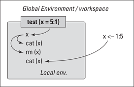
If R sees any object name — in this case, x — mentioned in any code in the function, it first searches the local environment. Because it finds an object x there, it uses that one for the first cat() statement. In the next line, R removes that object x. So, when R reaches the third line, it can’t find an object x in the local environment anymore. No problem. R moves up the stack of environments and checks to see if it finds anything looking like an x in the global environment. Because it can find an x there, it uses that one in the second cat() statement.

If you use rm() inside a function, rm() will, by default, delete only objects within that function. This way, you can avoid running out of memory when you write functions that have to work on huge datasets. You can immediately remove big temporary objects instead of waiting for the function to do so at the end.

Using internal functions

Writing your functions in such a way that they need objects in the global environment doesn’t really make sense, because you use functions to avoid dependency on objects in the global environment in the first place.

In fact, the whole concept behind R strongly opposes using global variables used in different functions. As a functional programming language, one of the main ideas of R is that the outcome of a function should not be dependent on anything but the values for the arguments of that function. If you give the arguments the same values, you always get the same result. If you come from other programming languages like Java, this characteristic may strike you as odd, but it has its merits. Sometimes you need to repeat some calculations a few times within a function, but these calculations only make sense inside that function.

Suppose you want to compare the light production of some lamps at half power and full power. The towels you put in front of the window to block the sun out aren’t really up to the job, so you also measure how much light is still coming through. You want to subtract the mean of this value from the results in order to correct your measurements.

To calculate the efficiency at 50 percent power, you can use the following function:

calculate.eff <- function(x, y, control){

  min.base <- function(z) z - mean(control)

  min.base(x) / min.base(y)

}

Inside the calculate.eff() function, you see another function definition for a min.base() function. Exactly as in the case of other objects, this function is created in the local environment of calculate.eff() and destroyed again when the function is done. You won’t find min.base() back in the workspace.

You can use the function as follows:

> half <- c(2.23, 3.23, 1.48)

> full <- c(4.85, 4.95, 4.12)

> nothing <- c(0.14, 0.18, 0.56, 0.23)

> calculate.eff(half, full, nothing)

[1] 0.4270093 0.6318887 0.3129473

If you look a bit more closely at the function definition of min.base(), you notice that it uses an object control but doesn’t have an argument with that name. How does this work then? When you call the function, the following happens (see Figure 8-2):

1. The function calculate.eff() creates a new local environment that contains the objects x (with the value of fifty), y (with the value of hundred), control (with the value of nothing), as well as the function min.base().

2. The function min.base() creates a new local environment within the one of calculate.eff() containing only one object z with the value of x.

3. min.base() looks for the object control in the environment of calculate.eff() and subtracts the mean of this vector from every number of z. This value is then returned.

4. The same thing happens again, but this time z gets the value of y.

5. Both results are divided by another, and the result is passed on to the global environment again.

The local environment is embedded in the environment where the function is defined, not where it’s called. Suppose you use addPercent() inside calculate.eff() to format the numbers. The local environment created by addPercent() is not embedded in the one of calculate.eff() but in the global environment, where addPercent() is defined.

Dispatching to a Method

We want to cover one more thing about functions, because you need it to understand how one function can give a different result based on the type of value you give the arguments. R has a genius system, called the generic function system, that allows you to call different functions using the same name. If you think this is weird, think again about data frames and lists (see Chapter 7). If you print a list in the console, you get the output arranged in rows. On the other hand, a data frame is printed to the console arranged in columns. So, the print() function treats lists and data frames differently, but both times you used the same function. Or did you really?

Finding the methods behind the function

It’s easy to find out if you used the same function both times — you can just peek inside the function code of print() by typing its name at the command line, like this:

> print

function (x, ...)

UseMethod(“print”)

<bytecode: 0x0464f9e4>

<environment: namespace:base>

You can safely ignore the two last lines, because they refer to complicated stuff in the “outer space” of R and are used only by R developers. But take a look at the function body — it’s only one line!

Functions that don’t do much other than passing on objects to the right function are called generic functions. In this example, print() is a generic function. The functions that do the actual work are called methods. So, every method is a function, but not every function is a method.

Using methods with UseMethod

How on earth can that one line of code in the print() function do so many complex things like printing vectors, data frames, and lists all in a different way? The answer is contained in the UseMethod() function, which is the central function in the generic function system of R. All UseMethod() does is tell R to move along and look for a function that can deal with the type of object that is given as the argument x.

R does that by looking through the complete set of functions in search of another function that starts with print followed by a dot and then the name of the object type.

You can do that yourself by using the command apropos(‘print\.’). Between the quotation marks, you can put a regular expression much like in the grep() function we discuss in Chapter 5. In order to tell R that the dot really means a dot, you have to precede it with two backslashes. Don’t be surprised when you get over 40 different print() functions for all kinds of objects.

Suppose you have a data frame you want to print. R will look up the function print.data.frame() and use that function to print the object you passed as an argument. You also can call that function yourself like this:

> small.one <- data.frame(a = 1:2, b = 2:1)

> print.data.frame(small.one)

  a b

1 1 2

2 2 1

The effect of that function differs in no way from what you would get if you used the generic print(small.one) function instead. That’s because print() will give the small.one to the print.data.frame() function to take care of it.

Using default methods

In the case of a list, you may be tempted to look for a print.list() function. But it won’t work, because the print.list() function doesn’t exist. Still that isn’t a problem for R — R will ignore the type of the object in that case and just look for a default method, print.default().

For many generic functions, there is a default method that’s used if no specific method can be found. If there is one, you can recognize the default method by the word default after the dot in the function name.

So, if you want to print the data frame as a list, you can use the default method like this:

> print.default(small.one)

$a

[1] 1 2

$b

[1] 2 1

attr(,”class”)

[1] “data.frame”

Doing it yourself

All that method dispatching sounds nice, but it may seem mostly like internal affairs of R and not that interesting to know as a user . . . unless you could use that system yourself, of course — and you can!

Adapting the addPercent function

Suppose you want to be able to paste the percent sign to character vectors with the addPercent function. As the function is written in the previous sections, you can’t. A character vector will give an error the moment you try to multiply it, so you need another function for that, like the following:

addPercent.character <- function(x){

  paste(x,”%”,sep=””)

}

Note that the type of the object is not vector but character. In the same way, you also have to rename the original addPercent function to addPercent.numeric in your script.

If you use the system of method dispatching, you can keep all functions in one script file if they aren’t too big. That way, you have to source only one script file in order to have the whole generic system working.

All you need now is a generic addPercent() function like this:

addPercent <- function(x,...){

  UseMethod(“addPercent”)

}

You use only two arguments here: x and the dots (...). The use of the dots argument assures you can still use all the arguments from the addPercent.numeric() function in your call to addPercent(). The extra arguments are simply passed on to the appropriate method via the dots argument, as explained in the “Using Arguments the Smart Way” section, earlier in this chapter.

After sending the complete script file to the console, you can send both character vectors and numeric vectors to addPercent(), like this:

> addPercent(new.numbers, FUN = floor)

[1] “82%”  “2%”   “162%” “40%”

> addPercent(letters[1:6])

[1] “a%” “b%” “c%” “d%” “e%” “f%”

Adding a default function

If you try to use the small data frame you made in the previous section, you would get the following error:

> addPercent(small.one)

Error in UseMethod(“addPercent”) :

  no applicable method for ‘addPercent’ applied to an object of class “data.frame”

That’s a rather complicated way of telling you that there’s no method for a data frame. There’s no need for a data frame method either, but it may be nice to point out to the users of your code that they should use a vector instead. So, you can easily add a default method exactly like R does:

addPercent.default <- function(x){

  cat(‘You should try a numeric or character vector. ’)

}

This default method doesn’t do much apart from printing a message, but at least that message is a bit easier to understand than the one R spits out. Sometimes it’s apparent that the error messages of R aren’t always written with a normal end-user in mind.