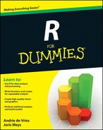
Figure 13-1: Different ways of combining data.
Chapter 13
Manipulating and Processing Data
In This Chapter
![]() Creating subsets of data
Creating subsets of data
![]() Adding calculated fields
Adding calculated fields
![]() Merging data from different sources
Merging data from different sources
![]() Sorting data
Sorting data
![]() Meeting more members of the apply family
Meeting more members of the apply family
![]() Getting your data into shape
Getting your data into shape
Now it’s time to put together all the tools that you encounter in earlier chapters. You know how to get data into R, you know how to work with lists and data frames, and you know how to write functions. Combined, these tools form the basic toolkit to be able to do data manipulation and processing in R.
In this chapter, you get to use some tricks and design idioms for working with data. This includes methods for selecting and ordering data, such as working with lookup tables. You also get to use some techniques for reshaping data — for example, changing the shape of data from wide format to long format.
Deciding on the Most Appropriate Data Structure
The first decision you have to make before analyzing your data is how to represent that data inside R. In Chapters 4, 5, and 7, you see that the basic data structures in R are vectors, matrices, lists, and data frames.
If your data has only one dimension, then you already know that vectors represent this type of data very well. However, if your data has more than one dimension, you have the choice of using matrices, lists, or data frames. So, the question is: When do you use which?
Matrices and higher-dimensional arrays are useful when all your data are of a single class — in other words, all your data are numeric or all your data are characters. If you’re a mathematician or statistician, you’re familiar with matrices and likely use this type of object very frequently.
But in many practical situations, you’ll have data that have many different classes — in other words, you’ll have a mixture of numeric and character data. In this case, you need to use either lists or data frames.
If you imagine your data as a single spreadsheet, a data frame is probably a good choice. Remember that a data frame is simply a list of named vectors of the same length, which is conceptually very similar to a spreadsheet with columns and a column heading for each. If you’re familiar with databases, you can think of a data frame as similar to a single table in a database. Data frames are tremendously useful and, in many cases, will be your first choice of objects for storing your data.
If your data consists of a collection of objects but you can’t represent that as an array or a data frame, then a list is your ideal choice. Because lists can contain all kinds of other objects, including other lists or data frames, they’re tremendously flexible. Consequently, R has a wide variety of tools to process lists.
Table 13-1 contains a summary of these choices.
 You may find that a data frame is a very suitable choice for most analysis and data-processing tasks. It’s a very convenient way of representing your data, and it’s similar to working with database tables. When you read data from a comma-separated value (CSV) file with the function
 read.csv() or read.table(), R puts the results in a data frame.
Table 13-1 Useful Objects for Data Analysis
|
Object |
Description |
Comments |
|
|
The basic data object in R, consisting of one or more values of a single type (for example, character, number, or integer). |
Think of this as a single column or row in a spreadsheet, or a column in a database table. |
|
|
A multidimensional object of a single type (known as atomic). A matrix is an array of two dimensions. |
When you have to store numbers in many dimensions, use arrays. |
|
|
Lists can contain objects of any type. |
Lists are very useful for storing collections of data that belong together. Because lists can contain lists, this type of object is very useful. |
|
|
Data frames are a special kind of named list where all the elements have the same length. |
Data frames are similar to a single spreadsheet or to a table in a database. |
Creating Subsets of Your Data
Often the first task in data processing is to create subsets of your data for further analysis. In Chapters 3 and 4, we show you ways of subsetting vectors. In Chapter 7, we outline methods for creating subsets of arrays, data frames, and lists.
Because this is such a fundamental task in data analysis, we review and summarize the different methods for creating subsets of data.
Understanding the three subset operators
 You’re already familiar with the three subset operators:
![]()
$: The dollar-sign operator selects a single element of your data (and drops the dimensions of the returned object). When you use this operator with a data frame, the result is always a vector; when you use it with a named list, you get that element.
![]()
[[: The double-square-brackets operator also returns a single element, but it offers you the flexibility of referring to the elements by position, rather than by name. You use it for data frames and lists.
![]()
[: The single-square-brackets operator can return multiple elements of your data.
This summary is simplified. Next, we look at how to use these operators to get exactly the elements from your data that you want.
Understanding the five ways of specifying the subset
When you use the single-square-brackets operator, you return multiple elements of your data. This means that you need a way of specifying exactly which elements you need.
In this paragraph, you can try subsetting with the built-in dataset islands, a named numeric vector with 48 elements.
> str(islands)
Named num [1:48] 11506 5500 16988 2968 16 ...
- attr(*, “names”)= chr [1:48] “Africa” “Antarctica” “Asia” “Australia” ...
Table 13-2 illustrates the five ways of specifying which elements you want to include in or exclude from your data.
Table 13-2 Specifying the Subset Elements
|
Subset |
Effect |
Example |
|
Blank |
Returns all your data |
|
|
Positive numerical values |
Extracts the elements at these locations |
|
|
Negative numerical values |
Extract all but these elements; in other words, excludes these elements |
|
|
Logical values |
A logical value of |
|
|
Text strings |
Includes elements where the names match |
|
Subsetting data frames
Now that you’ve reviewed the rules for creating subsets, you can try it with some data frames. You just have to remember that a data frame is a two-dimensional object and contains rows as well as columns. This means that you need to specify the subset for rows and columns independently. To do so, you combine the operators.
To illustrate subsetting of data frames, have a look at the built-in dataset iris, a data frame of five columns and 150 rows with data about iris flowers.
> str(iris)
‘data.frame’: 150 obs. of 5 variables:
$ Sepal.Length: num 5.1 4.9 4.7 4.6 5 5.4 4.6 5 4.4 4.9 ...
$ Sepal.Width : num 3.5 3 3.2 3.1 3.6 3.9 3.4 3.4 2.9 3.1 ...
$ Petal.Length: num 1.4 1.4 1.3 1.5 1.4 1.7 1.4 1.5 1.4 1.5 ...
$ Petal.Width : num 0.2 0.2 0.2 0.2 0.2 0.4 0.3 0.2 0.2 0.1 ...
$ Species : Factor w/ 3 levels “setosa”,”versicolor”,..: 1 1 1 1 1 1 1 1 1 1 ...
When you subset objects with more than one dimension, you specify the subset argument for each dimension — you separate the subset arguments with commas.
For example, to get the first five rows of iris and all the columns, try the following:
> iris[1:5, ]
To get all the rows but only two of the columns, try the following:
> iris[, c(“Sepal.Length”, “Sepal.Width”)]
You need to take special care when subsetting in a single column of a data frame. Try the following:
iris[, ‘Sepal.Length’]
You’ll see that the result is a vector, not a data frame as you would expect.
When your subset operation returns a single column, the default behavior is to return a simplified version. The way this works, is that R inspects the lengths of the returned elements. If all these elements have the same length, then R simplifies the result to a vector, matrix, or array. In our example, R simplifies the result to a vector. To override this behavior, you need to specify the argument drop=FALSE in your subset operation:
> iris[, ‘Sepal.Length’, drop=FALSE]
Alternatively, you can subset the data frame like a list, as shown in Chapter 7. The following code returns you a data frame with only one column as well:
> iris[‘Sepal.Length’]
Finally, to get a subset of only some columns and some rows:
> iris[1:5, c(“Sepal.Length”, “Sepal.Width”)]
Sepal.Length Sepal.Width
1 5.1 3.5
2 4.9 3.0
3 4.7 3.2
4 4.6 3.1
5 5.0 3.6
Taking samples from data
Statisticians often have to take samples of data and then calculate statistics. Because a sample is really nothing more than a subset of data, taking a sample is easy with R. To do so, you make use of sample(), which takes a vector as input; then you tell it how many samples to draw from that list.
Say you wanted to simulate rolls of a die, and you want to get ten results. Because the outcome of a single roll of a die is a number between one and six, your code looks like this:
> sample(1:6, 10, replace=TRUE)
[1] 2 2 5 3 5 3 5 6 3 5
You tell sample() to return ten values, each in the range 1:6. Because every roll of the die is independent from every other roll of the die, you’re sampling with replacement. This means that you take one sample from the list and reset the list to its original state (in other words, you put the element you’ve just drawn back into the list). To do this, you add the argument replace=TRUE, as in the example.
Because the return value of the sample() function is a randomly determined number, if you try this function repeatedly, you’ll get different results every time. This is the correct behavior in most cases, but sometimes you may want to get repeatable results every time you run the function. Usually, this will occur only when you develop and test your code, or if you want to be certain that someone else can test your code and get the same values you did. In this case, it’s customary to specify a so-called seed value.
 If you provide a seed value, the random-number sequence will be reset to a known state. This is because R doesn’t create truly random numbers, but only pseudo-random numbers. A pseudo-random sequence is a set of numbers that, for all practical purposes, seem to be random but were generated by an algorithm. When you set a starting seed for a pseudo-random process, R always returns the same pseudo-random sequence. But if you don’t set the seed, R draws from the current state of the random number generator (RNG). On startup R may set a random seed to initialize the RNG, but each time you call it, R starts from the next value in the RNG stream. You can read the Help for
 ?RNG to get more detail.
In R, you use the set.seed() function to specify your seed starting value. The argument to set.seed() is any integer value.
> set.seed(1)
> sample(1:6, 10, replace=TRUE)
[1] 2 3 4 6 2 6 6 4 4 1
If you draw another sample, without setting a seed, you get a different set of results, as you would expect:
> sample(1:6, 10, replace=TRUE)
[1] 2 2 5 3 5 3 5 6 3 5
Now, to demonstrate that set.seed() actually does reset the RNG, try it again. But this time, set the seed once more:
> set.seed(1)
> sample(1:6, 10, replace=TRUE)
[1] 2 3 4 6 2 6 6 4 4 1
You get exactly the same results as the first time you used set.seed(1).
You can use sample() to take samples from the data frame iris. In this case, you may want to use the argument replace=FALSE. Because this is the default value of the replace argument, you don’t need to write it explicitly:
> set.seed(123)
> index <- sample(1:nrow(iris), 5)
> index
[1] 44 119 62 133 142
> iris[index, ]
Sepal.Length Sepal.Width Petal.Length Petal.Width Species
44 5.0 3.5 1.6 0.6 setosa
119 7.7 2.6 6.9 2.3 virginica
62 5.9 3.0 4.2 1.5 versicolor
133 6.4 2.8 5.6 2.2 virginica
142 6.9 3.1 5.1 2.3 virginica
Removing duplicate data
A very useful application of subsetting data is to find and remove duplicate values.
R has a useful function, duplicated(), that finds duplicate values and returns a logical vector that tells you whether the specific value is a duplicate of a previous value. This means that for duplicated values, duplicated() returns FALSE for the first occurrence and TRUE for every following occurrence of that value, as in the following example:
> duplicated(c(1,2,1,3,1,4))
[1] FALSE FALSE TRUE FALSE TRUE FALSE
If you try this on a data frame, R automatically checks the observations (meaning, it treats every row as a value). So, for example, with the data frame iris:
> duplicated(iris)
[1] FALSE FALSE FALSE FALSE FALSE FALSE FALSE FALSE FALSE
[10] FALSE FALSE FALSE FALSE FALSE FALSE FALSE FALSE FALSE
....
[136] FALSE FALSE FALSE FALSE FALSE FALSE FALSE TRUE FALSE
[145] FALSE FALSE FALSE FALSE FALSE FALSE
If you look carefully, you notice that row 143 is a duplicate (because the 143rd element of your result has the value TRUE). You also can tell this by using the which() function:
> which(duplicated(iris))
[1] 143
Now, to remove the duplicate from iris, you need to exclude this row from your data. Remember that there are two ways to exclude data using subsetting:
![]() Specify a logical vector, where
Specify a logical vector, where FALSE means that the element will be excluded. The ! (exclamation point) operator is a logical negation. This means that it converts TRUE into FALSE and vice versa. So, to remove the duplicates from iris, you do the following:
> iris[!duplicated(iris), ]
![]() Specify negative values. In other words:
Specify negative values. In other words:
> index <- which(duplicated(iris))
> iris[-index, ]
In both cases, you’ll notice that your instruction has removed row 143.
Removing rows with missing data
Another useful application of subsetting data frames is to find and remove rows with missing data. The R function to check for this is complete.cases(). You can try this on the built-in dataset airquality, a data frame with a fair amount of missing data:
> str(airquality)
> complete.cases(airquality)
The results of complete.cases() is a logical vector with the value TRUE for rows that are complete, and FALSE for rows that have some NA values. To remove the rows with missing data from airquality, try the following:
> x <- airquality[complete.cases(airquality), ]
> str(x)
Your result should be a data frame with 111 rows, rather than the 153 rows of the original airquality data frame.
As always with R, there is more than one way of achieving your goal. In this case, you can make use of na.omit() to omit all rows that contain NA values:
> x <- na.omit(airquality)
When you’re certain that your data is clean, you can start to analyze it by adding calculated fields.
If you use any of these methods to subset your data or clean out missing values, remember to store the result in a new object. R doesn’t change anything in the original data frame unless you explicitly overwrite it. That’s a good thing, because you can’t accidently mess up your data.
Adding Calculated Fields to Data
After you’ve created the appropriate subset of your data, the next step in your analysis is likely to be to perform some calculations.
Doing arithmetic on columns of a data frame
R makes it very easy to perform calculations on columns of a data frame because each column is itself a vector. This means that you can use all the tools that you encountered in Chapters 4, 5, and 6.
Sticking to the iris data frame, try to do a few calculations on the columns. For example, calculate the ratio between the lengths and width of the sepals:
> x <- iris$Sepal.Length / iris$Sepal.Width
Now you can use all the R tools to examine your result. For example, inspect the first five elements of your results with the head() function:
> head(x)
[1] 1.457143 1.633333 1.468750 1.483871 1.388889 1.384615
As you can see, performing calculations on columns of a data frame is straightforward. Just keep in mind that each column is really a vector, so you simply have to remember how to perform operations on vectors (see Chapter 5).
Using with and within to improve code readability
After a short while of writing subset statements in R, you’ll get tired of typing the dollar sign to extract columns of a data frame. Fortunately, there is a way to reduce the amount of typing and to make your code much more readable at the same time. The trick is to use the with() function. Try this:
> y <- with(iris, Sepal.Length / Sepal.Width)
The with() function allows you to refer to columns inside a data frame without explicitly using the dollar sign or even the name of the data frame itself. So, in our example, because you use with(iris, ...) R knows to evaluate both Sepal.Length and Sepal.Width in the context of iris.
Hopefully, you agree that this is much easier to read and understand. By printing the values of your new variable y, you can confirm that it’s identical to x in the previous example.
> head(y)
[1] 1.457143 1.633333 1.468750 1.483871 1.388889 1.384615
You also can use the identical() function to get R to tell you whether these values are, in fact, the same:
> identical(x, y)
[1] TRUE
In addition to with(), the helpful within() function allows you to assign values to columns in your data very easily. Say you want to add your calculated ratio of sepal length to width to the original data frame. You’re already familiar with writing it like this:
> iris$ratio <- iris$Sepal.Length / iris$Sepal.Width
Now, using within() it turns into the following:
> iris <- within(iris, ratio <- Sepal.Length / Sepal.Width)
This works in a very similar way to with(), except that you can use the assign operator (<-) inside your function. If you now look at the structure of iris, you’ll notice that ratio is a column:
> head(iris$ratio)
[1] 1.457143 1.633333 1.468750 1.483871 1.388889 1.384615
Next, we take a look at how to cut your data into subgroups.
Creating subgroups or bins of data
One of the first tasks statisticians often use to investigate their data is to draw histograms. (You get to plot histograms in Chapter 15). A histogram is a plot of the number of occurrences of data in specific bins or subgroups. Because this type of calculation is fairly common when you do statistics, R has some functions to do exactly that.
The cut() function creates bins of equal size (by default) in your data and then classifies each element into its appropriate bin.
If this sounds like a mouthful, don’t worry. A few examples should make this come to life.
Using cut to create a fixed number of subgroups
To illustrate the use of cut(), have a look at the built-in dataset state.x77, an array with several columns and one row for each state in the United States:
> head(state.x77)
Population Income Illiteracy Life Exp Murder HS Grad Frost Area
Alabama 3615 3624 2.1 69.05 15.1 41.3 20 50708
Alaska 365 6315 1.5 69.31 11.3 66.7 152 566432
Arizona 2212 4530 1.8 70.55 7.8 58.1 15 113417
Arkansas 2110 3378 1.9 70.66 10.1 39.9 65 51945
California 21198 5114 1.1 71.71 10.3 62.6 20 156361
Colorado 2541 4884 0.7 72.06 6.8 63.9 166 103766
We want to work with the column called Frost. To extract this column, try the following:
> frost <- state.x77[, “Frost”]
> head(frost, 5)
Alabama Alaska Arizona Arkansas California
20 152 15 65 20
You now have a new object, frost, a named numeric vector. Now use cut() to create three bins in your data:
> cut(frost, 3, include.lowest=TRUE)
[1] [-0.188,62.6] (125,188] [-0.188,62.6] (62.6,125]
[5] [-0.188,62.6] (125,188] (125,188] (62.6,125]
....
[45] (125,188] (62.6,125] [-0.188,62.6] (62.6,125]
[49] (125,188] (125,188]
Levels: [-0.188,62.6] (62.6,125] (125,188]
The result is a factor with three levels. The names of the levels seem a bit complicated, but they tell you in mathematical set notation what the boundaries of your bins are. For example, the first bin contains those states that have frost between –0.188 and 62.8 days. In reality, of course, none of the states will have frost on negative days — R is being mathematically conservative and adds a bit of padding.
Note the argument include.lowest=TRUE to cut(). The default value for this argument is include.lowest=FALSE, which can sometimes cause R to ignore the lowest value in your data.
Adding labels to cut
The level names aren’t very user friendly, so specify some better names with the labels argument:
> cut(frost, 3, include.lowest=TRUE, labels=c(“Low”, “Med”, “High”))
[1] Low High Low Med Low High High Med Low Low Low
....
[45] High Med Low Med High High
Levels: Low Med High
Now you have a factor that classifies states into low, medium, and high, depending on the number of days of frost they get.
Using table to count the number of observations
One interesting piece of analysis is to count how many states are in each bracket. You can do this with the table() function, which simply counts the number of observations in each level of your factor.
> x <- cut(frost, 3, include.lowest=TRUE, labels=c(“Low”, “Med”, “High”))
> table(x)
x
Low Med High
11 19 20
You encounter the table() function again in Chapter 15.
Combining and Merging Data Sets
Now you have a grasp of how to subset your data and how to perform calculations on it. The next thing you may want to do is combine data from different sources. Generally speaking, you can combine different sets of data in three ways:
![]() By adding columns: If the two sets of data have an equal set of rows, and the order of the rows is identical, then adding columns makes sense. Your options for doing this are
By adding columns: If the two sets of data have an equal set of rows, and the order of the rows is identical, then adding columns makes sense. Your options for doing this are data.frame or cbind() (see Chapter 7).
![]() By adding rows: If both sets of data have the same columns and you want to add rows to the bottom, use
By adding rows: If both sets of data have the same columns and you want to add rows to the bottom, use rbind() (see Chapter 7).
![]() By combining data with different shapes: The
By combining data with different shapes: The merge() function combines data based on common columns, as well as common rows. In databases language, this is usually called joining data.
Figure 13-1 shows these three options schematically.
In this section, we look at some of the possibilities of combining data with merge(). More specifically, you use merge() to find the intersection, as well as the union, of different data sets. You also look at other ways of working with lookup tables, using the functions match() and %in%.

Sometimes you want to combine data where it isn’t as straightforward to simply add columns or rows. It could be that you want to combine data based on the values of preexisting keys in the data. This is where the merge() function is useful. You can use merge() to combine data only when certain matching conditions are satisfied.
Say, for example, you have information about states in a country. If one dataset contains information about population and another contains information about regions, and both have information about the state name, you can use merge() to combine your results.
Creating sample data to illustrate merging
To illustrate the different ways of using merge, have a look at the built-in dataset state.x77. This is an array, so start by converting it into a data frame. Then add a new column with the names of the states. Finally, remove the old row names. (Because you explicitly add a column with the names of each state, you don’t need to have that information duplicated in the row names.)
> all.states <- as.data.frame(state.x77)
> all.states$Name <- rownames(state.x77)
> rownames(all.states) <- NULL
Now you should have a data frame all.states with 50 observations of nine variables:
> str(all.states)
‘data.frame’: 50 obs. of 9 variables:
$ Population: num 3615 365 2212 2110 21198 ...
$ Income : num 3624 6315 4530 3378 5114 ...
$ Illiteracy: num 2.1 1.5 1.8 1.9 1.1 0.7 1.1 0.9 1.3 2 ...
$ Life Exp : num 69 69.3 70.5 70.7 71.7 ...
$ Murder : num 15.1 11.3 7.8 10.1 10.3 6.8 3.1 6.2 10.7 13.9 ...
$ HS Grad : num 41.3 66.7 58.1 39.9 62.6 63.9 56 54.6 52.6 40.6 ...
$ Frost : num 20 152 15 65 20 166 139 103 11 60 ...
$ Area : num 50708 566432 113417 51945 156361 ...
$ Name : chr “Alabama” “Alaska” “Arizona” “Arkansas” ...
Creating a subset of cold states
Next, create a subset called cold.states consisting of those states with more than 150 days of frost each year, keeping the columns Name and Frost:
> cold.states <- all.states[all.states$Frost>150, c(“Name”, “Frost”)]
> cold.states
Name Frost
2 Alaska 152
6 Colorado 166
....
45 Vermont 168
50 Wyoming 173
Creating a subset of large states
Finally, create a subset called large.states consisting of those states with a land area of more than 100,000 square miles, keeping the columns Name and Area:
> large.states <- all.states[all.states$Area>=100000, c(“Name”, “Area”)]
> large.states
Name Area
2 Alaska 566432
3 Arizona 113417
....
31 New Mexico 121412
43 Texas 262134
Now you’re ready to explore the different types of merge.
Using the merge() function
In R you use the merge() function to combine data frames. This powerful function tries to identify columns or rows that are common between the two different data frames.
Using merge to find the intersection of data
The simplest form of merge() finds the intersection between two different sets of data. In other words, to create a data frame that consists of those states that are cold as well as large, use the default version of merge():
> merge(cold.states, large.states)
Name Frost Area
1 Alaska 152 566432
2 Colorado 166 103766
3 Montana 155 145587
4 Nevada 188 109889
If you’re familiar with a database language such as SQL, you may have guessed that merge() is very similar to a database join. This is, indeed, the case and the different arguments to merge() allow you to perform natural joins, as well as left, right, and full outer joins.
The merge() function takes quite a large number of arguments. These arguments can look quite intimidating until you realize that they form a smaller number of related arguments:
![]()
x: A data frame.
![]()
y: A data frame.
![]()
by, by.x, by.y: The names of the columns that are common to both x and y. The default is to use the columns with common names between the two data frames.
![]()
all, all.x, all.y: Logical values that specify the type of merge. The default value is all=FALSE (meaning that only the matching rows are returned).
That last group of arguments — all, all.x and all.y — deserves some explanation. These arguments determine the type of merge that will happen (see the next section).
Understanding the different types of merge
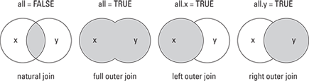
The merge() function allows four ways of combining data:
![]() Natural join: To keep only rows that match from the data frames, specify the argument
Natural join: To keep only rows that match from the data frames, specify the argument all=FALSE.
![]() Full outer join: To keep all rows from both data frames, specify
Full outer join: To keep all rows from both data frames, specify all=TRUE.
![]() Left outer join: To include all the rows of your data frame
Left outer join: To include all the rows of your data frame x and only those from y that match, specify all.x=TRUE.
![]() Right outer join: To include all the rows of your data frame
Right outer join: To include all the rows of your data frame y and only those from x that match, specify all.y=TRUE.
You can see a visual depiction of all these different options in Figure 13-2.
Figure 13-2: Different types of merge() and their database join equivalents.
Finding the union (full outer join)
Returning to the examples of U.S. states, to perform a complete merge of cold and large states, use merge and specify all=TRUE:
> merge(cold.states, large.states, all=TRUE)
Name Frost Area
1 Alaska 152 566432
2 Arizona NA 113417
3 California NA 156361
....
13 Texas NA 262134
14 Vermont 168 NA
15 Wyoming 173 NA
Both data frames have a variable Name, so R matches the cases based on the names of the states. The variable Frost comes from the data frame cold.states, and the variable Area comes from the data frame large.states.
Note that this performs the complete merge and fills the columns with NA values where there is no matching data.
Working with lookup tables
Sometimes doing a full merge of the data isn’t exactly what you want. In these cases, it may be more appropriate to match values in a lookup table. To do this, you can use the match() or %in% function.
Finding a match
The match() function returns the matching positions of two vectors or, more specifically, the positions of first matches of one vector in the second vector. For example, to find which large states also occur in the data frame cold.states, you can do the following:
> index <- match(cold.states$Name, large.states$Name)
> index
[1] 1 4 NA NA 5 6 NA NA NA NA NA
As you see, the result is a vector that indicates matches were found at positions one, four, five, and six. You can use this result as an index to find all the large states that are also cold states.
Keep in mind that you need to remove the NA values first, using na.omit():
> large.states[na.omit(index), ]
Name Area
2 Alaska 566432
6 Colorado 103766
26 Montana 145587
28 Nevada 109889
Making sense of %in%
A very convenient alternative to match() is the function %in%, which returns a logical vector indicating whether there is a match.
The %in% function is a special type of function called a binary operator. This means you use it by placing it between two vectors, unlike most other functions where the arguments are in parentheses:
> index <- cold.states$Name %in% large.states$Name
> index
[1] TRUE TRUE FALSE FALSE TRUE TRUE FALSE FALSE FALSE FALSE FALSE
If you compare this to the result of match(), you see that you have a TRUE value for every non-missing value in the result of match(). Or, to put it in R code, the operator %in% does the same as the following code:
> !is.na(match(cold.states$Name,large.states$Name))
[1] TRUE TRUE FALSE FALSE TRUE TRUE FALSE FALSE FALSE FALSE FALSE
The match() function returns the indices of the matches in the second argument for the values in the first argument. On the other hand, %in% returns TRUE for every value in the first argument that matches a value in the second argument. The order of the arguments is important here.
Because %in% returns a logical vector, you can use it directly to index values in a vector.
> cold.states[index, ]
Name Frost
2 Alaska 152
6 Colorado 166
26 Montana 155
28 Nevada 188
As we mention earlier, the %in% function is an example of a binary operator in R. This means that the function is used by putting it between two values, as you would for other operators, such as + (plus) and - (minus). At the same time, %in% is in infix operator. An infix operator in R is identifiable by the percent signs around the function name. If you want to know how %in% is defined, look at the details section of its Help page. But note that you have to place quotation marks around the function name to get the Help page, like this: ?”%in%”.
Sorting and Ordering Data
One very common task in data analysis and reporting is sorting information. You can answer many everyday questions with league tables — sorted tables of data that tell you the best or worst of specific things. For example, parents want to know which school in their area is the best, and businesses need to know the most productive factories or the most lucrative sales areas. When you have the data, you can answer all these questions simply by sorting it.
As an example, look again at the built-in data about the states in the U.S. First, create a data frame called some.states that contains information contained in the built-in variables state.region and state.x77:
> some.states <- data.frame(
+ Region = state.region,
+ state.x77)
To keep the example manageable, create a subset of only the first ten rows and the first three columns:
> some.states <- some.states[1:10, 1:3]
> some.states
Region Population Income
Alabama South 3615 3624
Alaska West 365 6315
Arizona West 2212 4530
....
Delaware South 579 4809
Florida South 8277 4815
Georgia South 4931 4091
You now have a variable called some.states that is a data frame consisting of ten rows and three columns (Region, Population, and Income).
Sorting vectors
R makes it easy to sort vectors in either ascending or descending order. Because each column of a data frame is a vector, you may find that you perform this operation quite frequently.
Sorting a vector in ascending order
To sort a vector, you use the sort() function. For example, to sort Population in ascending order, try this:
> sort(some.states$Population)
[1] 365 579 2110 2212 2541 3100 3615 4931 8277
[10] 21198
Sorting a vector in decreasing order
You also can tell sort() to go about its business in decreasing order. To do this, specify the argument decreasing=TRUE:
> sort(some.states$Population, decreasing=TRUE)
[1] 21198 8277 4931 3615 3100 2541 2212 2110 579
[10] 365
You can access the Help documentation for the sort() function by typing ?sort into the R console.
Sorting data frames
Another way of sorting data is to determine the order that elements should be in, if you were to sort. This sounds long winded, but as you’ll see, having this flexibility means you can write statements that are very natural.
Getting the order
First, determine the element order to sort state.info$Population in ascending order. Do this using the order() function:
> order.pop <- order(some.states$Population)
> order.pop
[1] 2 8 4 3 6 7 1 10 9 5
This means to sort the elements in ascending order, you first take the second element, then the eighth element, then the fourth element, and so on. Try it:
> some.states$Population[order.pop]
[1] 365 579 2110 2212 2541 3100 3615 4931 8277
[10] 21198
Yes, this is rather long winded. But next we look at how you can use order() in a very powerful way to sort a data frame.
Sorting a data frame in ascending order
In the preceding section, you calculated the order in which the elements of Population should be in order for it to be sorted in ascending order, and you stored that result in order.pop. Now, use order.pop to sort the data frame some.states in ascending order of population:
> some.states[order.pop, ]
Region Population Income
Alaska West 365 6315
Delaware South 579 4809
Arkansas South 2110 3378
....
Georgia South 4931 4091
Florida South 8277 4815
California West 21198 5114
Sorting in decreasing order
Just like sort(), the order() function also takes an argument called decreasing. For example, to sort some.states in decreasing order of population:
> order(some.states$Population)
[1] 2 8 4 3 6 7 1 10 9 5
> order(some.states$Population, decreasing=TRUE)
[1] 5 9 10 1 7 6 3 4 8 2
Just as before, you can sort the data frame some.states in decreasing order of population. Try it, but this time don’t assign the order to a temporary variable:
> some.states[order(some.states$Population, decreasing=TRUE), ]
Region Population Income
California West 21198 5114
Florida South 8277 4815
Georgia South 4931 4091
....
Arkansas South 2110 3378
Delaware South 579 4809
Alaska West 365 6315
Sorting on more than one column
You probably think that sorting is very straightforward, and you’re correct. Sorting on more than one column is almost as easy.
You can pass more than one vector as an argument to the order() function. If you do so, the result will be the equivalent of adding a secondary sorting key. In other words, the order will be determined by the first vector and any ties will then sort according to the second vector.
Next, you get to sort some.states on more than one column — in this case, Region and Population. If this sounds confusing, don’t worry — it really isn’t. Try it yourself. First, calculate the order to sort some.states in the order of region as well at population:
> index <- with(some.states, order(Region, Population))
> some.states[index, ]
Region Population Income
Connecticut Northeast 3100 5348
Delaware South 579 4809
Arkansas South 2110 3378
Alabama South 3615 3624
Georgia South 4931 4091
Florida South 8277 4815
Alaska West 365 6315
Arizona West 2212 4530
Colorado West 2541 4884
California West 21198 5114
Traversing Your Data with the Apply Functions
R has a powerful suite of functions that allows you to apply a function repeatedly over the elements of a list. The interesting and crucial thing about this is that it happens without an explicit loop. In Chapter 9, you see how to use loops appropriately and get a brief introduction to the apply family.
Because this is such a useful concept, you’ll come across quite a few different flavors of functions in the apply family of functions. The specific flavor of apply() depends on the structure of data that you want to traverse:
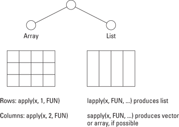
![]() Array or matrix: Use the
Array or matrix: Use the apply() function. This traverses either the rows or columns of a matrix, applies a function to each resulting vector, and returns a vector of summarized results.
![]() List: Use the
List: Use the lapply() function to traverse a list, apply a function to each element, and return a list of the results. Sometimes it’s possible to simplify the resulting list into a matrix or vector. This is what the sapply() function does.
Figure 13-3 demonstrates the appropriate function, depending on whether your data is in the form of an array or a list.
Figure 13-3: Use apply on arrays and matrices; use lapply or sapply on lists.
The ability to apply a function over the elements of a list is one of the distinguishing features of the functional programming style as opposed to an imperative programming style. In the imperative style, you use loops, but in the functional programming style you apply functions. R has a variety of apply-type functions, including apply(), lapply(), and sapply().
Using the apply() function to summarize arrays
If you have data in the form of an array or matrix and you want to summarize this data, the apply() function is really useful. The apply() function traverses an array or matrix by column or row and applies a summarizing function.
The apply() function takes four arguments:
![]()
X: This is your data — an array (or matrix).
![]()
MARGIN: A numeric vector indicating the dimension over which to traverse; 1 means rows and 2 means columns.
![]()
FUN: The function to apply (for example, sum or mean).
![]()
... (dots): If your FUN function requires any additional arguments, you can add them here.
To illustrate this, look at the built-in dataset Titanic. This is a four-dimensional table with passenger data of the ship Titanic, describing their cabin class, gender, age, and whether they survived.
> str(Titanic)
table [1:4, 1:2, 1:2, 1:2] 0 0 35 0 0 0 17 0 118 154 ...
- attr(*, “dimnames”)=List of 4
..$ Class : chr [1:4] “1st” “2nd” “3rd” “Crew”
..$ Sex : chr [1:2] “Male” “Female”
..$ Age : chr [1:2] “Child” “Adult”
..$ Survived: chr [1:2] “No” “Yes”
In Chapter 14, you find some more examples of working with tables, including information about how tables differ from arrays.
To find out how many passengers were in each of their cabin classes, you need to summarize Titanic over its first dimension, Class:
> apply(Titanic, 1, sum)
1st 2nd 3rd Crew
325 285 706 885
Similarly, to calculate the number of passengers in the different age groups, you need to apply the sum() function over the third dimension:
> apply(Titanic, 3, sum)
Child Adult
109 2092
You also can apply a function over two dimensions at the same time. To do this, you need to combine the desired dimensions with the c() function. For example, to get a summary of how many people in each age group survived, you do the following:
> apply(Titanic, c(3, 4), sum)
Survived
Age No Yes
Child 52 57
Adult 1438 654
Using lapply() and sapply() to traverse a list or data frame
In Chapter 9 we show you how to use the lapply() and sapply() functions. In this section, we briefly review these functions.
When your data is in the form of a list, and you want to perform calculations on each element of that list, the appropriate apply function is lapply(). For example, to get the class of each element of iris, do the following:
> lapply(iris, class)
As you know, when you use sapply(), R attempts to simplify the results to a matrix or vector:
> sapply(iris, class)
Sepal.Length Sepal.Width Petal.Length Petal.Width Species
“numeric” “numeric” “numeric” “numeric” “factor”
Say you want to calculate the mean of each column of iris:
> sapply(iris, mean)
Sepal.Length Sepal.Width Petal.Length Petal.Width Species
5.843333 3.057333 3.758000 1.199333 NA
Warning message:
In mean.default(X[[5L]], ...) :
argument is not numeric or logical: returning NA
There is a problem with this line of code. It throws a warning message because species is not a numeric column. So, you may want to write a small function inside apply() that tests whether the argument is numeric. If it is, then calculate the mean score; otherwise, simply return NA.
In Chapter 8, you create your own functions. The FUN argument of the apply() functions can be any function, including your own custom functions. In fact, you can go one step further. It’s actually possible to define a function inside the FUN argument call to any apply() function:
> sapply(iris, function(x) ifelse(is.numeric(x), mean(x), NA))
Sepal.Length Sepal.Width Petal.Length Petal.Width Species
5.843333 3.057333 3.758000 1.199333 NA
What’s happening here? You defined a function that takes a single argument x. If x is numeric, it returns mean(x); otherwise, it returns NA. Because sapply() traverses your list, each column, in turn, is passed to your function and evaluated.
When you define a nameless function like this inside another function, it’s called an anonymous function. Anonymous functions are useful when you want to calculate something fairly simple, but you don’t necessarily want to permanently store that function in your workspace.
Using tapply() to create tabular summaries
So far, you’ve used three members of the apply family of functions: apply(), lapply(), and sapply(). It’s time to meet the fourth member of the family. You use tapply() to create tabular summaries of data. This function takes three arguments:
![]()
X: A vector
![]()
INDEX: A factor or list of factors
![]()
FUN: A function
With tapply(), you can easily create summaries of subgroups in data. For example, calculate the mean sepal length in the dataset iris:
> tapply(iris$Sepal.Length, iris$Species, mean)
setosa versicolor virginica
5.006 5.936 6.588
With this short line of code, you do some powerful stuff. You tell R to take the Sepal.Length column, split it according to Species, and then calculate the mean for each group.
This is an important idiom for writing code in R, and it usually goes by the name Split, Apply, and Combine (SAC). In this case, you split a vector into groups, apply a function to each group, and then combine the result into a vector.
Of course, using the with() function, you can write your line of code in a slightly more readable way:
> with(iris, tapply(Sepal.Length, Species, mean))
setosa versicolor virginica
5.006 5.936 6.588
Using tapply(), you also can create more complex tables to summarize your data. You do this by using a list as your INDEX argument.
Using tapply() to create higher-dimensional tables
For example, try to summarize the data frame mtcars, a built-in data frame with data about motor-car engines and performance. As with any object, you can use str() to inspect its structure:
> str(mtcars)
The variable am is a numeric vector that indicates whether the engine has an automatic (0) or manual (1) gearbox. Because this isn’t very descriptive, start by creating a new object, cars, that is a copy of mtcars, and change the column am to be a factor:
> cars <- within(mtcars,
+ am <- factor(am, levels=0:1, labels=c(“Automatic”, “Manual”))
+ )
Now use tapply() to find the mean miles per gallon (mpg) for each type of gearbox:
> with(cars, tapply(mpg, am, mean))
Automatic Manual
17.14737 24.39231
Yes, you’re correct. This is still only a one-dimensional table. Now, try to make a two-dimensional table with the type of gearbox (am) and number of gears (gear):
> with(cars, tapply(mpg, list(gear, am), mean))
Automatic Manual
3 16.10667 NA
4 21.05000 26.275
5 NA 21.380
You use tapply() to create tabular summaries of data. This is a little bit similar to the table() function. However, table() can create only contingency tables (that is, tables of counts), whereas with tapply() you can specify any function as the aggregation function. In other words, with tapply(), you can calculate counts, means, or any other value.
If you want to summarize statistics on a single vector, tapply() is very useful and quick to use.
Using aggregate()
Another R function that does something very similar is aggregate():
> with(cars, aggregate(mpg, list(gear=gear, am=am), mean))
gear am x
1 3 Automatic 16.10667
2 4 Automatic 21.05000
3 4 Manual 26.27500
4 5 Manual 21.38000
Next, you take aggregate() to new heights using the formula interface.
Getting to Know the Formula Interface
Now it’s time to get familiar with another very important idea in R: the formula interface. The formula interface allows you to concisely specify which columns to use when fitting a model, as well as the behavior of the model.
It’s important to keep in mind that the formula notation refers to statistical formulae, as opposed to mathematical formulae. So, for example, the formula operator + means to include a column, not to mathematically add two columns together. Table 13-3 contains some formula operators, as well as examples and their meanings. You need these operators when you start building models.
We won’t go deeper into this subject in this book, but now you know what to look for in the Help pages of different modeling functions. Be aware of the fact that the interpretation of the signs can differ depending on the modeling function you use.
Table 13-3 Some Formula Operators and Their Meanings
|
Operator |
Example |
Meaning |
|
|
|
Model |
|
|
|
Include columns |
|
|
|
Include |
|
|
|
Estimate the interaction of |
|
|
y |
Include columns as well as their interaction (that is, |
|
|
|
Estimate |
Many R functions allow you to use the formula interface, often in addition to other ways of working with that function. For example, the aggregate() function also allows you to use formulae:
> aggregate(mpg ~ gear + am, data=cars, mean)
gear am mpg
1 3 Automatic 16.10667
2 4 Automatic 21.05000
3 4 Manual 26.27500
4 5 Manual 21.38000
Notice that the first argument is a formula and the second argument is the source data frame. In this case, you tell aggregate to model mpg as a function of gear as well as am and to calculate the mean. This is the same example as in the previous paragraph, but by using the formula interface your function becomes very easy to read.
When you look at the Help file for a function, it’ll always be clear whether you can use a formula with that function. For example, take a look at the Help for ?aggregate. In the usage section of this page, you find the following text:
## S3 method for class ‘data.frame’
aggregate(x, by, FUN, ..., simplify = TRUE)
## S3 method for class ‘formula’
aggregate(formula, data, FUN, ...,
subset, na.action = na.omit)
This page lists a method for class data.frame, as well as a method for class formula. This indicates that you can use either formulation.
You can find more (technical) information about formula on its own Help page, ?formula.
In the next section, we offer yet another example of using the formula interface for reshaping data.
Whipping Your Data into Shape
Often, a data analysis task boils down to creating tables with summary information, such as aggregated totals, counts, or averages. Say, for example, you have information about four games of Granny, Geraldine, and Gertrude:
Game Venue Granny Geraldine Gertrude
1 1st Bruges 12 5 11
2 2nd Ghent 4 4 5
3 3rd Ghent 5 2 6
4 4th Bruges 6 4 7
You now want to analyze the data and get a summary of the total scores for each player in each venue:
variable Bruges Ghent
1 Granny 18 9
2 Geraldine 9 6
3 Gertrude 18 11
If you use spreadsheets, you may be familiar with the term pivot table. The functionality in pivot tables is essentially the ability to group and aggregate data and to perform calculations.
In the world of R, people usually refer to this as the process of reshaping data. In base R, there is a function, reshape(), that does this, but we discuss how to use the add-on package reshape2, which you can find on CRAN.
Understanding data in long and wide format
When talking about reshaping data, it’s important to recognize data in long and wide formats. These visual metaphors describe two ways of representing the same information.
You can recognize data in wide format by the fact that columns generally represent groups. So, our example of basketball games is in wide format, because there is a column for the baskets made by each of the participants
Game Venue Granny Geraldine Gertrude
1 1st Bruges 12 5 11
2 2nd Ghent 4 4 5
3 3rd Ghent 5 2 6
4 4th Bruges 6 4 7
In contrast, have a look at the long format of exactly the same data:
Game Venue variable value
1 1st Bruges Granny 12
2 2nd Ghent Granny 4
3 3rd Ghent Granny 5
4 4th Bruges Granny 6
5 1st Bruges Geraldine 5
6 2nd Ghent Geraldine 4
7 3rd Ghent Geraldine 2
8 4th Bruges Geraldine 4
9 1st Bruges Gertrude 11
10 2nd Ghent Gertrude 5
11 3rd Ghent Gertrude 6
12 4th Bruges Gertrude 7
Notice how, in the long format, the three columns for Granny, Geraldine, and Gertrude have disappeared. In their place, you now have a column called value that contains the actual score and a column called variable that links the score to either of the three ladies.
When converting data between long and wide formats, it’s important to be able to distinguish identifier variables from measured variables:
![]() Identifier variables: Identifier, or ID, variables identify the observations. Think of these as the key that identifies your observations. (In database design, these are called primary or secondary keys.)
Identifier variables: Identifier, or ID, variables identify the observations. Think of these as the key that identifies your observations. (In database design, these are called primary or secondary keys.)
![]() Measured variables: This represents the measurements you observed.
Measured variables: This represents the measurements you observed.
In our example, the identifier variables are Game and Venue, while the measured variables are the goals (that is, the columns Granny, Geraldine, and Gertrude).
Getting started with the reshape2 package
Base R has a function, reshape(), that works fine for data reshaping. However, the original author of this function had in mind a specific use case for reshaping: so-called longitudinal data.
Longitudinal research takes repeated observations of a research subject over a period of time. For this reason, longitudinal data typically has the variables associated with time.
The problem of data reshaping is far more generic than simply dealing with longitudinal data. For this reason, Hadley Wickham wrote and released the package reshape2 that contains several functions to convert data between long and wide format.
To download and install reshape2, use install.packages():
> install.packages(“reshape2”)
At the start of each new R session that uses reshape2, you need to load the package into memory using library():
> library(“reshape2”)
Now you can start. First, create some data:
> goals <- data.frame(
+ Game = c(“1st”, “2nd”, “3rd”, “4th”),
+ Venue = c(“Bruges”, “Ghent”, “Ghent”, “Bruges”),
+ Granny = c(12, 4, 5, 6),
+ Geraldine = c(5, 4, 2, 4),
+ Gertrude = c(11, 5, 6, 7)
+ )
This constructs a wide data frame with five columns and four rows with the scores of Granny, Geraldine, and Gertrude.
Melting data to long format
You’ve already seen the words wide and long as visual metaphors for the shape of your data. In other words, wide data tends to have more columns and fewer rows compared to long data. The reshape package extends this metaphor by using the terminology of melt and cast:
![]() To convert wide data to long, you melt it with the
To convert wide data to long, you melt it with the melt() function.
![]() To convert long data to wide, you cast it with the
To convert long data to wide, you cast it with the dcast() function for data frames or the acast() function for arrays.
Try converting your wide data frame goals to a long data frame using melt():
> mgoals <- melt(goals)
Using Game, Venue as id variables
The melt() function tries to guess your identifier variables (if you don’t provide them explicitly) and tells you which ones it used. By default, it considers all categorical variables (that is, factors) as identifier variables. This is often a good guess, and it’s exactly what we want in our example.
Specifying your identifier variables explicitly is a good idea. You do this by adding an argument id.vars, where you specify the column names of the identifiers:
> mgoals <- melt(goals, id.vars=c(“Game”, “Venue”))
The new object, mgoals, now contains your data in long format:
> mgoals
Game Venue variable value
1 1st Bruges Granny 12
2 2nd Ghent Granny 4
3 3rd Ghent Granny 5
...
10 2nd Ghent Gertrude 5
11 3rd Ghent Gertrude 6
12 4th Bruges Gertrude 7
Casting data to wide format
Now that you have a molten dataset (a dataset in long format), you’re ready to reshape it. To illustrate that the process of reshaping keeps all your data intact, try to reconstruct the original:
> dcast(mgoals, Venue + Game ~ variable, sum)
Game Venue Granny Geraldine Gertrude
1 1st Bruges 12 5 11
2 2nd Ghent 4 4 5
3 3rd Ghent 5 2 6
4 4th Bruges 6 4 7
Can you see how dcast() takes a formula as its second argument? More about that in a minute, but first inspect your results. It should match the original data frame.
Next, you may want to do something more interesting — for example, create a summary by venue and player.
You use the dcast() function to cast a molten data frame. To be clear, you use this to convert from a long format to a wide format, but you also can use this to aggregate into intermediate formats, similar to the way a pivot table works.
The dcast() function takes three arguments:
![]()
data: A molten data frame.
![]()
formula: A formula that specifies how you want to cast the data. This formula takes the form x_variable ~ y_variable. But we simplified it to make a point. You can use multiple x-variables, multiple y-variables and even z-variables. We say more about that in a few paragraphs.
![]()
fun.aggregate: A function to use if the casting formula results in data aggregation (for example, length(), sum(), or mean()).
So, to get that summary of venue versus player, you need to use dcast() with a casting formula variable ~ Venue. Note that the casting formula refers to columns in your molten data frame:
> dcast(mgoals, variable ~ Venue , sum)
variable Bruges Ghent
1 Granny 18 9
2 Geraldine 9 6
3 Gertrude 18 11
If you want to get a table with the venue running down the rows and the player across the columns, your casting formula should be Venue ~ variable:
> dcast(mgoals, Venue ~ variable , sum)
Venue Granny Geraldine Gertrude
1 Bruges 18 9 18
2 Ghent 9 6 11
It’s actually possible to have more complicated casting formulae. According to the Help page for dcast(), the casting formula takes this format:
x_variable + x_2 ~ y_variable + y_2 ~ z_variable ~ ...
Notice that you can combine several variables in each dimension with the plus sign (+), and you separate each dimension with a tilde (~). Also, if you have two or more tildes in the formula (that is, you include a z-variable), your result will be a multidimensional array.
So, to get a summary of goals by Venue, player (variable), and Game, you do the following:
> dcast(mgoals, Venue + variable ~ Game , sum)
Venue variable 1st 2nd 3rd 4th
1 Bruges Granny 12 0 0 6
2 Bruges Geraldine 5 0 0 4
3 Bruges Gertrude 11 0 0 7
4 Ghent Granny 0 4 5 0
5 Ghent Geraldine 0 4 2 0
6 Ghent Gertrude 0 5 6 0
One of the reasons you should understand data in long format is that both of the graphics packages lattice and ggplot2 make extensive use of long format data. The benefit is that you can easily create plots of your data that compares different subgroups. For example, the following code generates Figure 13-4:
> library(ggplot2)
> ggplot(mgoals, aes(x=variable, y=value, fill=Game)) + geom_bar()
Figure 13-4: Data in long (molten) format makes it easy to work with ggplot graphics.

..................Content has been hidden....................
You can't read the all page of ebook, please click here login for view all page.