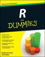
Figure 2-1: The shortcut icon for RGui is labeled with R followed by the version number.
Chapter 2
Exploring R
In This Chapter
![]() Looking at your R editing options
Looking at your R editing options
![]() Starting R
Starting R
![]() Writing your first R script
Writing your first R script
![]() Finding your way around the R workspace
Finding your way around the R workspace
In order to start working in R, you need to use an editing tool. Which editing tool you use depends to some extent on your operating system, because R doesn’t provide a single graphical editor for all operating systems. The basic R install gives you the following:
![]() Windows: A basic editor called RGui.
Windows: A basic editor called RGui.
![]() Mac OS X: A basic R editor called R.app.
Mac OS X: A basic R editor called R.app.
![]() Linux: There is no specific R editor on Linux, but you can use any editor (like Vim or Emacs) to edit your R code.
Linux: There is no specific R editor on Linux, but you can use any editor (like Vim or Emacs) to edit your R code.
At a practical level, this difference between operating systems doesn’t matter very much because R is a programming language, and you can be sure that R interprets your code identically across operating systems.
Still, we want to show you how to use an R code editor, so in this chapter we briefly illustrate how to use R with the Windows RGui. Our advice also works on R.app. And if you work in Linux, you can simply type the code into your preferred editor.
Fortunately, there is an alternative called RStudio, third-party software that provides a consistent user interface regardless of operating system. In addition to demonstrating how to work with the Windows RGui, we also illustrate how to use RStudio.
After you’ve opened a console, we get you exercising your R muscles and writing some scripts. You do some calculations, create some numeric and text variables, get to look at the built-in help, and save your work.
Working with a Code Editor
R is many things: a programming language, a statistical processing environment, a way to solve problems, and a collection of helpful tools to make your life easier. The one thing that R is not is an application, which means that you have the freedom of selecting your own editing tools to interact with R.
In this section we discuss the Windows R editor, RGui (short for R graphical user interface). Since the standard, basic R editors are so, well, basic, we also introduce you to RStudio. RStudio offers a richer editing environment than RGui and makes some common tasks easier and more fun.
Exploring RGui
As part of the process of downloading and installing R, you get the standard graphical user interface (GUI), called RGui. RGui gives you some tools to manage your R environment — most important, a console window. The console is where you type instructions, or scripts, and generally get R to do useful things for you.
Alternatives to the standard R editors
Among the many freedoms that R offers you is the freedom to choose your own code editor and development environment, so you don’t have to use the standard R editors or RStudio. Here are a few other options:
![]() Eclipse StatET (
Eclipse StatET (www.walware.de/goto/statet): Eclipse, another powerful integrated development environment, has a R add-in called StatET. If you’ve done software development on large projects, you may find Eclipse useful. Eclipse requires you to install Java on your computer.
![]() Emacs Speaks Statistics (
Emacs Speaks Statistics (http://ess.r-project.org): Emacs, a powerful text and code editor, is widely used in the Linux world and also is available for Windows. It has a statistics add-in called Emacs Speaks Statistics (ESS), which is famous for having keyboard shortcuts for just about everything you could possibly do and for its very loyal fan base. If you’re a programmer coming from the Linux world, this editor may be a good choice for you.
![]() Tinn-R (
Tinn-R (www.sciviews.org/Tinn-R): This editor, developed specifically for working with R, is available only for Windows. It has some nice features for setting up collections of R scripts in projects. Tinn-R is easier to install and use than either Eclipse or Emacs, but it isn’t as fully featured.
Seeing the naked R console
The standard installation process creates useful menu shortcuts (although this may not be true if you use Linux, because there is no standard RGui editor for Linux). In the menu system, look for a folder called R, and then find an icon called R followed by a version number (for example, R 2.13.2, as shown in Figure 2-1).
When you open RGui for the first time, you see the R Console screen (shown in Figure 2-2), which lists some basic information such as your version of R and the licensing conditions.
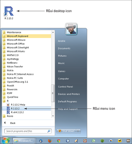
Figure 2-2: A brand-new session in RGui.
Below all this information is the R prompt, denoted by a > symbol. The prompt indicates where you type your commands to R; you see a blinking cursor to the right of the prompt.
We explore the R console in more depth in “Discovering the Workspace,” later in this chapter.
Issuing a simple command
Use the console to issue a very simple command to R. Type the following to calculate the sum of some numbers:
> 24+7+11
R responds immediately to your command, calculates the total, and displays it in the console:
> 24+7+11
[1] 42
The answer is 42. R gives you one other piece of information: The [1] preceding 42 indicates that the value 42 is the first element in your answer. It is, in fact, the only element in your answer! One of the clever things about R is that it can deal with calculating many values at the same time, which is called vector operations. We talk about vectors later in this chapter — for now, all you need to know is that R can handle more than one value at a time.
Closing the console
To quit your R session, type the following code in the console, after the command prompt (>):
> q()
R asks you a question to make sure that you meant to quit, as shown in Figure 2-3. Click No, because you have nothing to save. This action closes your R session (as well as RGui, if you’ve been using RGui as your code editor).
Figure 2-3: R asks you a simple question.

Dressing up with RStudio
RStudio is a code editor and development environment with some very nice features that make code development in R easy and fun:
![]() Code highlighting that gives different colors to keywords and variables, making it easier to read
Code highlighting that gives different colors to keywords and variables, making it easier to read
![]() Automatic bracket matching
Automatic bracket matching
![]() Code completion, so you don’t have to type out all commands in full
Code completion, so you don’t have to type out all commands in full
![]() Easy access to R Help, with some nice features for exploring functions and parameters of functions
Easy access to R Help, with some nice features for exploring functions and parameters of functions
![]() Easy exploration of variables and values
Easy exploration of variables and values
Because RStudio is available free of charge for Linux, Windows, and Apple iOS devices, we think it’s a good option to use with R. In fact, we like RStudio so much that we use it to illustrate the examples in this book. Throughout the book, you find some tips and tricks on how things can be done in RStudio. If you decide to use a different code editor, you can still use all the code examples and you’ll get identical results.
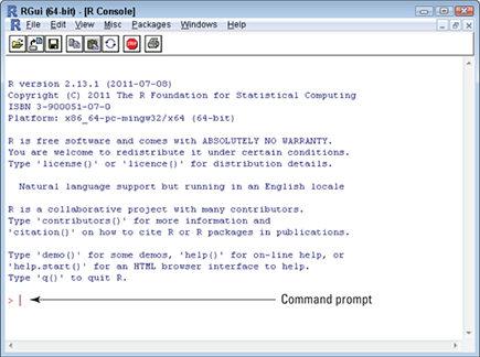
To open RStudio, click the RStudio icon in your menu system or on your desktop, as shown in Figure 2-4. (You can find installation instructions in this book’s appendix.)
Figure 2-4: Opening RStudio.
Once RStudio started, choose File⇒New⇒R Script.
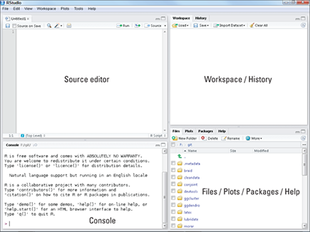
Your screen should look like Figure 2-5. You have four work areas:
![]() Source: The top-left corner of the screen contains a text editor that lets you work with source script files. Here, you can enter multiple lines of code, save your script file to disk, and perform other tasks on your script. This code editor works a bit like every other text editor you’ve ever seen, but it’s smart. It recognizes and highlights various elements of your code, for example (using different colors for different elements), and it also helps you find matching brackets in your scripts.
Source: The top-left corner of the screen contains a text editor that lets you work with source script files. Here, you can enter multiple lines of code, save your script file to disk, and perform other tasks on your script. This code editor works a bit like every other text editor you’ve ever seen, but it’s smart. It recognizes and highlights various elements of your code, for example (using different colors for different elements), and it also helps you find matching brackets in your scripts.
![]() Console: In the bottom-left corner, you find the console. The console in RStudio is identical to the console in RGui (refer to “Seeing the naked R console,” earlier in this chapter). This is where you do all the interactive work with R.
Console: In the bottom-left corner, you find the console. The console in RStudio is identical to the console in RGui (refer to “Seeing the naked R console,” earlier in this chapter). This is where you do all the interactive work with R.
![]() Workspace and history: The top-right corner is a handy overview of your workspace, where you can inspect the variables you created in your session, as well as their values. (We discuss the workspace in more detail later in this chapter.) This is also the area where you can see a history of the commands you’ve issued in R.
Workspace and history: The top-right corner is a handy overview of your workspace, where you can inspect the variables you created in your session, as well as their values. (We discuss the workspace in more detail later in this chapter.) This is also the area where you can see a history of the commands you’ve issued in R.
![]() Files, plots, package, and help: In the bottom-right corner, you have access to several tools:
Files, plots, package, and help: In the bottom-right corner, you have access to several tools:
• Files: This is where you can browse the folders and files on your computer.
• Plots: This is where R displays your plots (charts or graphs). We discuss plots in Part V.
• Packages: This is where you can view a list of all the installed packages. A package is self-contained set of code that adds functionality to R, similar to the way that an add-in adds functionality to Microsoft Excel.
• Help: This is where you can browse the built-in Help system of R.
Figure 2-5: RStudio’s four work areas.
Starting Your First R Session
If you’re anything like the two of us, you’re probably just itching to get hold of some real code. In this section, you get to do exactly that. Get ready to get your hands dirty!
Saying hello to the world
Programming books typically start with a very simple program. Often, the objective of this first program is to create the message “Hello world!” In R, this program consists of one line of code.
Start a new R session, type the following in your console, and press Enter:
> print(“Hello world!”)
R responds immediately with this output:
[1] “Hello world!”
Congratulations! You’ve just completed your first R script.
 As we explain in the introduction to this book, we collapse these two things into a single block of code, like this:
> print(“Hello world!”)
[1] “Hello world!”
Doing simple math
Type the following in your console to calculate the sum of five numbers:
> 1+2+3+4+5
[1] 15
The answer is 15, which you can easily verify for yourself. You may think that there’s an easier way to calculate this value, though — and you’d be right. We explain how in the following section.
Using vectors
A vector is the simplest type of data structure in R. The R manual defines a vector as “a single entity consisting of a collection of things.” A collection of numbers, for example, is a numeric vector — the first five integer numbers form a numeric vector of length 5.
To construct a vector, type the following in the console:
> c(1,2,3,4,5)
[1] 1 2 3 4 5
In constructing your vector, you have successfully used a function in R. In programming language, a function is a piece of code that takes some inputs and does something specific with them. In constructing a vector, you tell the c() function to construct a vector with the first five integers. The entries inside the parentheses are referred to as arguments.
You also can construct a vector by using operators. An operator is a symbol you stick between two values to make a calculation. The symbols +, -, *, and / are all operators, and they have the same meaning they do in mathematics. Thus, 1+2 in R returns the value 3, just as you’d expect.
One very handy operator is called sequence, and it looks like a colon (:). Type the following in your console:
> 1:5
[1] 1 2 3 4 5
That’s more like it. With three keystrokes, you’ve generated a vector with the values 1 through 5. Type the following in your console to calculate the sum of this vector:
> sum(1:5)
[1] 15
Storing and calculating values
Using R as a calculator is very interesting but perhaps not all that useful. A much more useful capability is storing values and then doing calculations on these stored values.
Try the following:
> x <- 1:5
> x
[1] 1 2 3 4 5
In these two lines of code, you first assign the sequence 1:5 to a variable called x. Then you ask R to print the value of x by typing x in the console and pressing Enter.
In R, the assignment operator is <-, which you type in the console by using two keystrokes: the less-than symbol (<) followed by a hyphen (-). The combination of these two symbols represents assignment.
In addition to retrieving the value of a variable, you can do calculations on that value. Create a second variable called y, and assign it the value 10. Then add the values of x and y, as follows:
> y <- 10
> x + y
[1] 11 12 13 14 15
The values of the two variables themselves don’t change unless you assign a new value. You can check this by typing the following:
> x
[1] 1 2 3 4 5
> y
[1] 10
Now create a new variable z, assign it the value of x+y, and print its value:
> z <- x + y
> z
[1] 11 12 13 14 15
Variables also can take on text values. You can assign the value “Hello” to a variable called h, for example, by presenting the text to R inside quotation marks, like this:
> h <- “Hello”
> h
[1] “Hello”
You must present text or character values to R inside quotation marks — either single or double. R accepts both. So both h <- “Hello” and h <- ‘Hello’ are examples of valid R syntax.
In “Using vectors,” earlier in this chapter, you use the c() function to combine numeric values into vectors. This technique also works for text. Try it:
> hw <- c(“Hello”, “world!”)
> hw
[1] “Hello” “world!”
You can use the paste() function to concatenate multiple text elements. By default, paste() puts a space between the different elements, like this:
> paste(“Hello”, “world!”)
[1] “Hello world!”
Talking back to the user
You can write R scripts that have some interaction with a user. To ask the user questions, you can use the readline() function. In the following code snippet, you read a value from the keyboard and assign it to the variable yourname:
> h <- “Hello”
> yourname <- readline(“What is your name?”)
What is your name?Andrie
> paste(h, yourname)
[1] “Hello Andrie”
This code seems to be a bit cumbersome, however. Clearly, it would be much better to send these three lines of code simultaneously to R and get them evaluated in one go. In the next section, we show you how.
Sourcing a Script
Until now, you’ve worked directly in the R console and issued individual commands in an interactive style of coding. In other words, you issue a command, R responds, you issue the next command, R responds, and so on.
In this section, you kick it up a notch and tell R to perform several commands one after the other without waiting for additional instructions. Because the R function to run an entire script is source(), R users refer to this process as sourcing a script.
To prepare your script to be sourced, you first write the entire script in an editor window. In RStudio, for example, the editor window is in the top-left corner of the screen (refer to Figure 2-5). Whenever you press Enter in the editor window, the cursor moves to the next line, as in any text editor.
Type the following lines of code in the editor window. (Remember that in RStudio the source editor is in the top-left corner, by default.) Notice that the last line contains a small addition to the code you saw earlier: the print() function.
h <- “Hello”
yourname <- readline(“What is your name?”)
print(paste(h, yourname))
Remember to type the print() function as part of your script. Sourced scripts behave differently from interactive code in printing results. In interactive mode, a result is printed even without a print() function. But when you source a script, output is printed only if you have an explicit print() function.
You can type multiple lines of code into the source editor without having each line evaluated by R. Then, when you’re ready, you can send the instructions to R — in other words, source the script.
When you use RGui or RStudio, you can do this in one of three ways:
![]() Send an individual line of code from the editor to the console. Click the line of code you want to run, and then press Ctrl+R in RGui. In RStudio, you can press Ctrl+Enter or click the Run button.
Send an individual line of code from the editor to the console. Click the line of code you want to run, and then press Ctrl+R in RGui. In RStudio, you can press Ctrl+Enter or click the Run button.
![]() Send a block of highlighted code to the console. Select the block of code you want to run, and then press Ctrl+R (in RGui) or Ctrl+Enter (in RStudio).
Send a block of highlighted code to the console. Select the block of code you want to run, and then press Ctrl+R (in RGui) or Ctrl+Enter (in RStudio).
![]() Send the entire script to the console (which is called sourcing a script). In RGui, click anywhere in your script window, and then choose Edit⇒Run all. In RStudio, click anywhere in the source editor, and press Ctrl+Shift+Enter or click the Source button.
Send the entire script to the console (which is called sourcing a script). In RGui, click anywhere in your script window, and then choose Edit⇒Run all. In RStudio, click anywhere in the source editor, and press Ctrl+Shift+Enter or click the Source button.
These keyboard shortcuts are defined only in RStudio. If you use a different source editor, you may not have the same options.
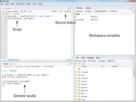
Now you can send the entire script to the R console. To do this, click the Source button in the top-right corner of the editor window or choose Edit⇒Source. The script starts, reaches the point where it asks for input, and then waits for you to enter your name in the console window. Your screen should now look like Figure 2-6. Notice that the Workspace window now lists the two objects you created: h and yourname.
Figure 2-6: Sending a script to the console in RStudio.
 When you click the Source button,
 source(‘~/.active-rstudio- document’) appears in the console. What RStudio actually does here is save your script in a temporary file and then use the R function source() to call that script in the console. Remember this function; you’ll meet it again.
Navigating the Workspace
So far in this chapter, you’ve created several variables. These form part of what R calls the workspace, which we explore in this section. The workspace refers to all the variables and functions (collectively called objects) that you create during the session, as well as any packages that are loaded.
Often, you want to remind yourself of all the variables you’ve created in the workspace. To do this, use the ls() function to list the objects in the workspace. In the console, type the following:
> ls()
[1] “h” “hw” “x” “y” “yourname” “z”
R tells you the names of all the variables that you created.
 One very nice feature of RStudio lets you examine the contents of the workspace at any time without typing any R commands. By default, the top-right window in RStudio has two tabs: Workspace and History. Click the Workspace tab to see the variables in your workspace, as well as their values. (refer to Figure 2-5).
Manipulating the content of the workspace
If you decide that you don’t need some variables anymore, you can remove them. Suppose that the object z is simply the sum of two other variables and no longer needed. To remove it permanently, use the rm() function and then use the ls() function to display the contents of the workspace, as follows:
> rm(z)
> ls()
[1] “h” “hw” “x” “y” “yourname”
Notice that the object z is no longer there.
Saving your work
You have several options for saving your work:
![]() You can save individual variables with the
You can save individual variables with the save() function.
![]() You can save the entire workspace with the
You can save the entire workspace with the save.image() function.
![]() You can save your R script file, using the appropriate save menu command in your code editor.
You can save your R script file, using the appropriate save menu command in your code editor.
Suppose you want to save the value of yourname. To do that, follow these steps:
1. Find out which working directory R will use to save your file by typing the following:
> getwd()
[1] “c:/users/andrie”
The default working directory should be your user folder. The exact name and path of this folder depend on your operating system. (In Chapter 12, you get more familiar with the working directory.)
If you use the Windows operating system, the path is displayed with slashes instead of backslashes. In R, similar to many other programming languages, the backslash character has a special meaning. The backslash indicates an escape sequence, indicating that the character following the backslash means something special. For example, indicates a tab, rather than the letter t. (You can read more about escape sequences in Chapter 12.) Rest assured that, although the working directory is displayed differently from what you’re used to, R is smart enough to translate it when you save or load files. Conversely, when you type a file path, you have to use slashes, not backslashes.
2. Type the following code in your console, using a filename like yourname.rda, and then press Enter.
> save(yourname, file=”yourname.rda”)
R silently saves the file in the working directory. If the operation is successful, you don’t get any confirmation message.
3. To make sure that the operation was successful, use your file browser to navigate to the working directory, and see whether the new file is there.
Retrieving your work
To retrieve saved data, you use the load() function. Say you want to retrieve the value of yourname that you saved previously.
First, remove the variable yourname, so you can see the effect of the load process:
> rm(yourname)
If you’re using RStudio, you may notice that yourname is no longer displayed in the Workspace.
Next, use load to retrieve your variable. Type load followed by the filename you used to save the value earlier:
> load(“yourname.rda”)
Notice that yourname reappears in the Workspace window of RStudio.
..................Content has been hidden....................
You can't read the all page of ebook, please click here login for view all page.