8

Nodes in Adobe Substance 3D Designer

Nodes are graph inputs and outputs, which are the main tools for creating substances inside Adobe Substance 3D Designer, and we will examine these nodes in this chapter. Adobe Substance 3D Designer provides a huge selection of nodes for the creation of graphs. There are so many nodes that listing them all on a single page would be infeasible.

As a result, we’ll review some of the nodes that are used the most. You will get the opportunity to discover more about these nodes in this chapter, as well as why they are so important and what purpose they serve.

We will cover the following topics in this chapter:

• Working with nodes and understanding the basics in Adobe Substance 3D Designer
• Tile Generator node
• Flood Fill node
• Quad Transform node
• Height Blend node
• Curve node
• Dirt and Dust node
• Shape Mapper node
• Shape Splatter node
• Histogram Scan

Working with nodes and understanding the basics in Adobe Substance 3D Designer

In the first section of this chapter, we will learn how the node system works inside Adobe Substance 3D Designer. As mentioned before, Adobe Substance 3D Designer contains a variety of nodes and the usage of these nodes differs between them, but you do not need to worry about that, as they are pretty much self-explanatory.

However, the first thing we need to know is how we can work with the nodes inside Adobe Substance 3D Design in a very simple way, so let’s do that:

1. Once Adobe Substance 3D Designer is launched, a welcome window will pop up, and from there, you can choose Substance graph under the Create option.
2. As soon you do so, the New Substance Graph window will open, and from there, you can choose Metallic Roughness from the TEMPLATES list because this contains all the useful premade nodes, which you can edit later.
3. Then, change the Graph Name details to whatever you want. We will name this project Node Tests. Make sure Output format is set to Relative to parent so that everything you produce uses the same format as the parent:

Figure 8.1 – Creating a new substance graph

4. You can also go to the File menu, select New, then choose Substance graph, and repeat step 2. The setup of all the basic output nodes will be inside the GRAPH window.
5. To test different nodes, let’s go to 3D VIEW, click on the Scene menu, and choose Plain (hi-res). We will select this Scene mesh because it is simple and easier to observe the results produced by different nodes:

Figure 8.2 – Changing the 3D VIEW scene to a hi-res plane

6. In the GRAPH window, you will see six input nodes, which you can replace with your own inputs, and six output nodes, which are the Metallic Roughness output nodes:
   • Base Color: This node defines the base color of the mesh or substance, often taking Uniform Color or Gradient as its input.
   • Normal: A grayscale input picture is interpreted as a height map and used by the Normal filter to produce a normal map. Normal maps also fake the height and produce a kind of height illusion, which is often used in games or films instead of Height or Tessellation + Displacement.
   • Roughness: This node defines the roughness of the material surface, often taking Uniform Color or Gradient as its input. If the Uniform Color option is dark, the material will become shinier like glossy plastic, glass, or metal, and if the Uniform Color option is lighter, the material will become matte like paper.
   • Metallic: This node defines how metallic the material is, often taking Uniform Color or Gradient as its input. If the Uniform Color option is darker (such as black), the material will not be reflective (like paper), and if the Uniform Color option is lighter (such as white), the material will be reflective (like chrome).
   • Height: This node takes a grayscale input and creates an output based on the blacks and whites – a whiter color will give more height while a blacker color will produce negative height, and a grayish color will keep the height flat. However, to enable it, you need to make a few discreet settings adjustments.
   • Ambient Occlusion: This node mimics the way light strikes an item. Although it affects all facets of the item, the shadow regions are where it is most obvious, often taking the same map used for the Height map as its input.
7. Now, drag Checker 1 from LIBRARY to the GRAPH window, as shown in Figure 8.3:

Figure 8.3 – Dragging the Checker 1 pattern to the GRAPH window

8. Now, delete the Uniform Color node from the Ambient Occlusion and Height map nodes so that we can use our own node:

Figure 8.4 – Deleting the existing Uniform Color nodes

9. Now, connect the Checker 1 node to Height so that it can produce the checker pattern height, and connect it to Ambient Occlusion too so that it can produce the shadow effects based on the checker pattern. Right-click anywhere in the GRAPH window and choose View Outputs In 3D View:

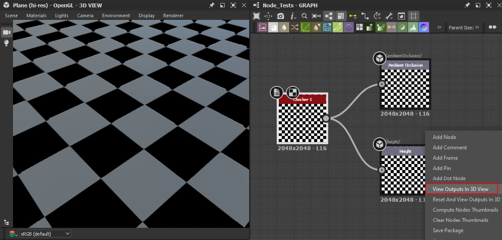
Figure 8.5 – Producing the Height map and Ambient Occlusion

10. Now, let us reveal the secret I spoke about in terms of the Height map node before. First of all, we can increase the height amount. However, to increase the height, the Scene mesh of our Plane needs a higher resolution, which is referred to as Tesselation in Adobe Substance 3D Designer. The height displacement here is specifically for helping visualize the material as you make it while it is inside of Adobe Substance 3D Designer.
11. Therefore, go to the Materials menu in 3D VIEW, select Default, then select Metallic Roughness, and choose Tesselation + Displacement:

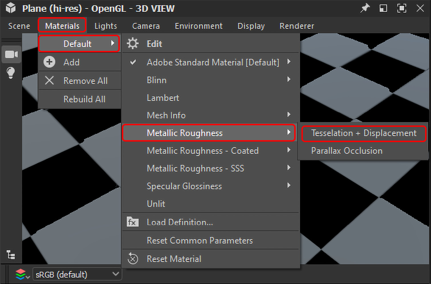
Figure 8.6 – Metallic Roughness material

12. Now that you have the Height parameters in the Properties window, you can increase the height of the Height map node by increasing the Height Scale value. Therefore, slide the Scale slider to the maximum, 10.

At first, it seems like you cannot increase the value to more than 10 through the slider. Nevertheless, you can type in a value greater than 10 using your keyboard.

13. To increase the resolution of the height map, you can type a higher value into Tessellation factor, so type in 16. Keep the Scalar Zero/Height Level value to 0.5. This slider actually sets the gray value:

Figure 8.7 – Material “Default” | OpenGL | PROPERTIES

14. To create a Normal map height, move the Normal map node next to the Checker 1 pattern node, and connect the Checker 1 pattern node to the Normal map node, as shown in Figure 8.8:

Figure 8.8 – Connecting the Checker 1 pattern node to the Normal map node

15. To organize the graph better, move the Base Color, Roughness, Metallic, and all Uniform Color nodes connected to them closer to the Checker 1 pattern node, as shown in Figure 8.9:

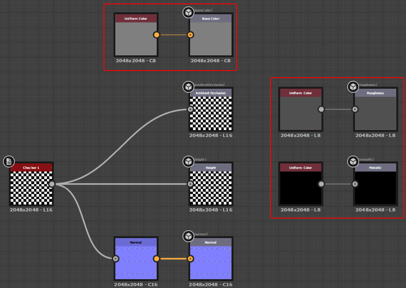
Figure 8.9 – Organizing the nodes

16. Double-click Base Color’s Uniform Color node so that its properties appear, keep Color Mode set to Color in the PROPERTIES window, and change it to whatever color you want. If they are already in the right color mode, you don’t need to apply any changes.
17. To give it a metallic look, change the Uniform Color mode of the Metallic node to Grayscale and change the color to white. To keep the metal shiny, change the Roughness node’s Uniform Color property to black:

Figure 8.10 – Changing the Base Color, Metallic, and Roughness nodes

Some nodes inside Adobe Substance 3D Designer are Color Mode-specific; the yellow and gray circle input link means it can take both Color and Grayscale outputs, and the yellow circle input link means it can only take Color outputs, while the gray circle input link means it can only take Grayscale outputs:

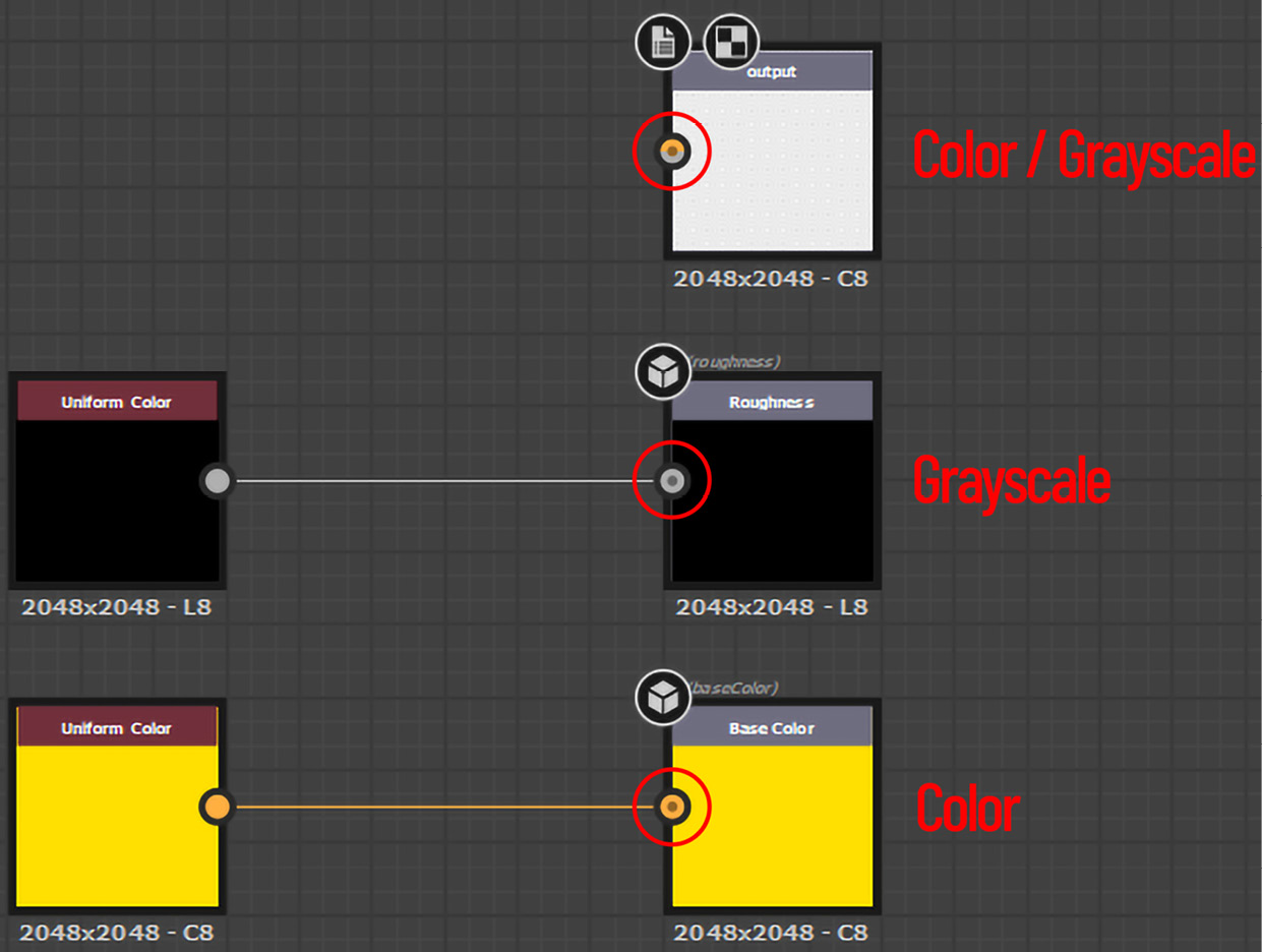
Figure 8.11 – Color Mode-specific links

Therefore, if you want to connect a Grayscale node to a Color input, you will get a red dotted line error, as shown in Figure 8.12:

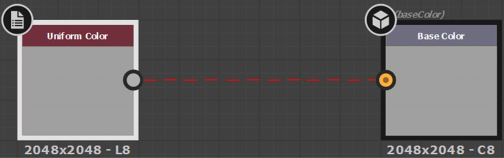
Figure 8.12 – Connecting different mode nodes

18. To avoid this error, you can select the red dotted line link and press the spacebar to get the Nodes menu. From the menu list, choose Gradient Map. This will convert the grayscale to color, as shown in Figure 8.13:

Figure 8.13 – Converting Grayscale to Color

19. Similarly, you can choose the Grayscale Conversion node if you want to input a Color node to a Grayscale node, as shown in Figure 8.13:

Figure 8.14 – Converting Color to Grayscale

20. Now, the issue is that if you re-open your project, your 3D settings will be reset even if you save it. Therefore, to avoid this, you have to go to 3D VIEW and click Scene.
21. Choose Save Current State and save it as Nodes_Test.sbsscn. You can also choose Save Current State As Default. However, it will become a default scene:

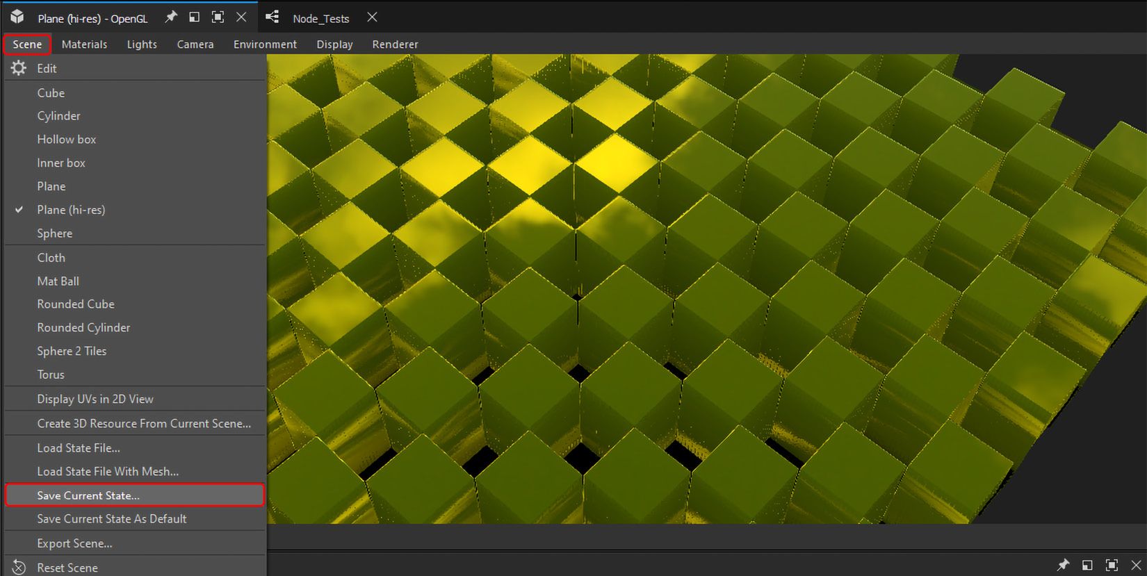
Figure 8.15 – Saving the current state

Save your graph and re-open it – you will notice that your 3D Scene has been reset.

22. To retain the saved state, go to 3D View, click on Scene | Load State File, choose Nodes_Test.sbsscn, and select your Scene Material, which was Plane (hi-res). This will load your saved state with all the settings:

Figure 8.16 – Loading a state file

Hopefully, you may have been familiar with the usage of nodes inside Adobe Substance 3D Designer. Now, let us go through the Atomic nodes, which are basically the most frequently used node.

Atomic nodes

A designer’s most fundamental building blocks are called Atomic nodes. There are 26 Atomic nodes in the older versions of Adobe Substance 3D Designer and 28 in the newer version, but we’ll just discuss the most commonly used ones here:

Figure 8.17 – Atomic nodes

• A – Blend: With a user-defined blend mode and an optional opacity mask, the Blend node combines or blends two distinct inputs. It is the most beneficial node in Designer and you will use it in practically every graph you create.

It’s comparable to stacking two layers one on top of the other in Painter or Photoshop and blending them using the top layer’s mode. Chapter 9, Blending Modes in Adobe Substance 3D Designer, is entirely based on this node.

• B – Uniform Color: A consistent, user-defined color or value is returned by the Uniform Color node. It is a straightforward node that is frequently used as a foundation for adding color or developing certain values. If you want to produce a shade of gray, convert this node to grayscale. Graphs are quicker to edit and perform better when in the grayscale color mode.
• C – Bitmap: The Bitmap node can be used to produce a bitmap for use with the 2D painting tools or to import an existing bitmap into your graph. This node should always be used in your graph if a bitmap file is required. Either start from scratch to construct the node or drop a bitmap in a suitable format into the graph view.
• D – Levels: You can remap the tones of input by configuring the input and output remap factors in the Levels node. The Levels node’s user interface is comparable to Photoshop’s levels tool. A Histogram preview is also available in the Levels node’s settings. One of the fundamental nodes in Substance Designer, the Levels node is frequently used to remap and modify values in a graph since it offers the most precise interface for doing so.
• E – Output: A unique node called an Output node acts as the finish line for your graphs. The input to Output nodes is not processed in any way. Only one input slot, which automatically switches between color and grayscale, is present on the Output node. In contrast to Input nodes, which offer properties that help you arrange your assets, output nodes lack parameters.

These are a few most commonly used Atomic nodes, in the later chapters we will study more about Atomic nodes, for the time being, let us study some useful Library nodes.

Library nodes

A library of graph instance nodes created by Atomic nodes is included with Designer. Some are designed for particular use circumstances, while others are frequently useful.

Figure 8.18 – Library nodes

We’ll have an overview of a few typical ones:

• A – Tile Generator: One of the library’s more sophisticated nodes is the Tile Generator node. When you master the tile generator, you can use it to make the majority of designs. Almost any graph can utilize the tile generator because it is very adaptable and doesn’t require patterns. Use custom shapes and parameter adjustments to generate an infinite number of variants.
• B – Flood Fill: Flood Fill is one of a sophisticated group of effects that let you give a simple binary tile texture a lot more diversity. It is more of a starting point for other Flood Fill effects and is not intended to be utilized alone.
• C – Quad Transform: A special transform node that interacts with the corner points of a quadrilateral shape to transform it. It allows for precise hands-on transformations.
• D – Height Blend: This is based on the height information of the two height maps combined. It creates a black and white mask that may be utilized anywhere in addition to a blended height map.
• E – Curve: As with other 2D image editing programs, the Curve node offers an interface for picture tone remapping. The input, which can either monochrome (grayscale) or colored, can be remapped by the user by placing points and adjusting Bezier curves.
• F – Dirt: This node creates a black and white mask using user parameters and baked maps, similar to Painter’s Smart Masks. This doesn’t need baked Ambient Occlusion (AO) – you can also use built-in AO and Curvature. This mask represents dirt on obscured and sunken edges and corners.
• G – Dust: This node creates a black and white mask using user parameters and baked maps, similar to Painter’s Smart Masks. This mask symbolizes dust that has gathered exclusively in places that face upward and in occluded, lowered locations. It only works with properly baked AO and World Space Normal. This doesn’t need baked AO – you can also use built-in AO and Curvature.
• H – Shape Mapper: This transforms and accurately maps an input pattern along a polygonal or circular route. It’s comparable to Splatter Circular, but with the form distortion which is necessary to precisely follow the course. When you want a height map to be twisted into a circle, for instance, it might be helpful in some very particular situations.
• I – Shape Splatter: Its primary function is to enable the insertion of forms on and inside a height map, which is then used to build different maps from the Splatter Data – for instance, arranging pebbles, twigs, and leaves on a landscape that is guided and orientated by different maps. Then, despite using the same common Splatter Data for all channels, different maps may be used for Height, Normal, Base Color, Roughness, and any other channel.
• J – Histogram Scan: A node that offers an easy way to remap the contrast and brightness of input grayscale photos – very basic yet helpful. It can be used to dynamically grow and shrink masks.
• K – Ambient Occlusion (HBAO/RTAO): This node converts a height map into an AO map by taking it as input. It employs the sophisticated technique known as Horizon-Based Ambient Occlusion (HBAO). It may be used to convert generative height maps into excellent AO maps. Although more computationally costly, a Ray Tracing Ambient Occlusion (RTAO) node is also offered.
• L – Blur HQ: A high-quality Gaussian blur is applied to the input by Blur HQ, precisely like the effect in Photoshop. While taking longer to calculate, it has a lot better quality than the typical atomic Blur node. The blur’s quality level can be altered using a node-specific option.
• M – Gaussian Noise: This node creates soft, straightforward random blobs on an adjustable scale, producing one of the most basic yet most useful noise maps. Additional parameters are available to add looping motion to the noise. Gaussian noise is frequently a wise choice if you are unsure of the noise to employ.

I hope the Atomic and Library nodes are clear to you, so let us use these nodes in practice. We will also go through some more common nodes while we will be working on them practically.

The Tile Generator node

As discussed before, the Tile Generator node helps you to create different types of tiles using different shapes. In this section, we will create brick-shaped tiles, and we will also learn how to work with Gradient Map.

1. Open Node_Tests.sbs in Adobe Substance 3D Designer, go to 3D View | Load State File, choose Nodes_Test.sbsscn from the Scene menu, and choose Plane (hi-res).

Now, we need to replace the existing Checker Map node with Tile Generator.

2. To do that, click inside the GRAPH window with your left-hand mouse button and press the spacebar to load the nodes library. Type Tile Generator into the search field and select the Tile Generator node.
3. Remove the Checker Map node and connect the Tile Generator node with the existing nodes, as shown in Figure 8.19:

Figure 8.19 – Adding a Tile Generator node

4. Right-click with your mouse inside the GRAPH window and choose View Outputs In 3D View.
5. Double-click on the Tile Generator node and once its properties start showing in the PROPERTIES window, adjust the following settings:
   • INSTANCE PARAMETERS: X Amount: 5, Y Amount: 15
   • Position: Offset: 0.5 Offset Random: 0.1

This will create a brick-shaped tile with a little randomness, as shown in Figure 8.20:

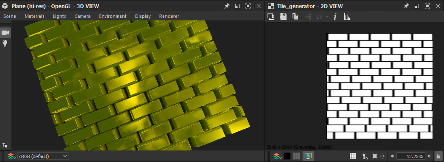
Figure 8.20 – A brick-shaped tile

6. You will notice that the height value is too much for the brick map. Therefore, go to 3D VIEW, click on the Materials menu, select the Default option, and choose Edit.
7. Once the material parameters have loaded in the PROPERTIES window, change the height scale to 1.5, as shown in Figure 8.21.

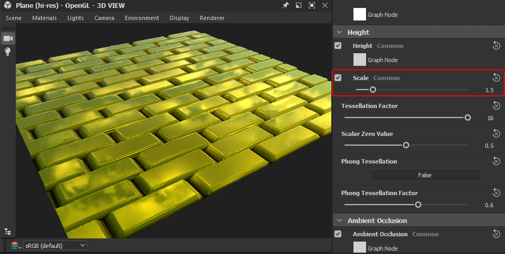
Figure 8.21 – Changing the height

8. Now, let us give the brick tile some realistic color. Therefore, we will not use Uniform Color this time; we will use Gradient Map with the Noise node that matches the brick tile. So, disconnect Uniform Color from Base Color, remove Uniform Color, and add Gradient Map instead, as shown in Figure 8.22:

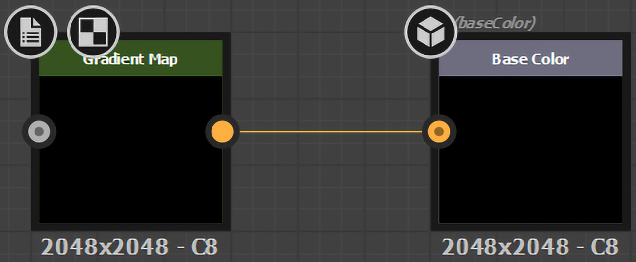
Figure 8.22 – Gradient Map

9. The gradient map needs a node that has variation, such as a Noise node, to generate a gradient. Therefore, we will add Grunge Concrete and connect it to Base Color. After that, double-click Grunge Concrete and change its Balance to 0.55 and Contrast to 3.5:

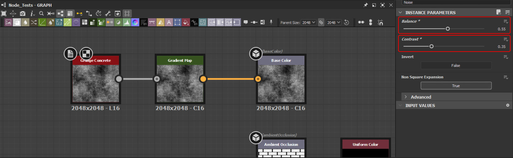
Figure 8.23 – Adding Gradient Concrete

10. Now, go to your internet browser and load any high-resolution red brick image, keep the internet browser and the Adobe Substance 3D Designer window open side by side, and execute the following steps:
    1. Double-click Gradient Map to load its parameters inside the PROPERTIES window.
    2. Go to the Gradient Map’s properties and click Gradient Editor.
    3. Once the Gradient Editor window opens, click Pick Gradient.
    4. Once you click Pick Gradient, you will load a Gradient Picker Cursor. Therefore, with that cursor, drag across the red brick image with your left-hand mouse button held down, as shown in Figure 8.24:

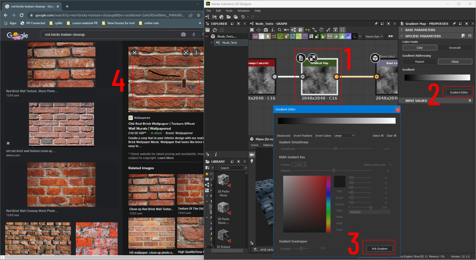
Figure 8.24 – Picking a gradient

11. Now, change the Roughness node’s Uniform Color property to white and the Metallic node’s Uniform Color property to black. These colors will make the brick look rougher, without any reflective quality, like real bricks:

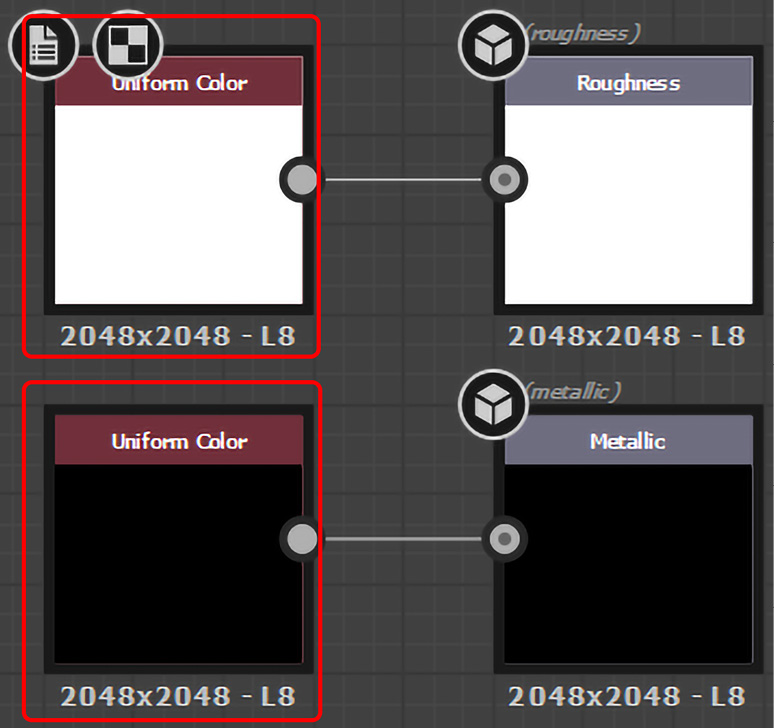
Figure 8.25 – Changing the Color properties for the Roughness and Metallic nodes

Now, you will have a much more realistic-looking red brick wall, as shown in Figure 8.26:

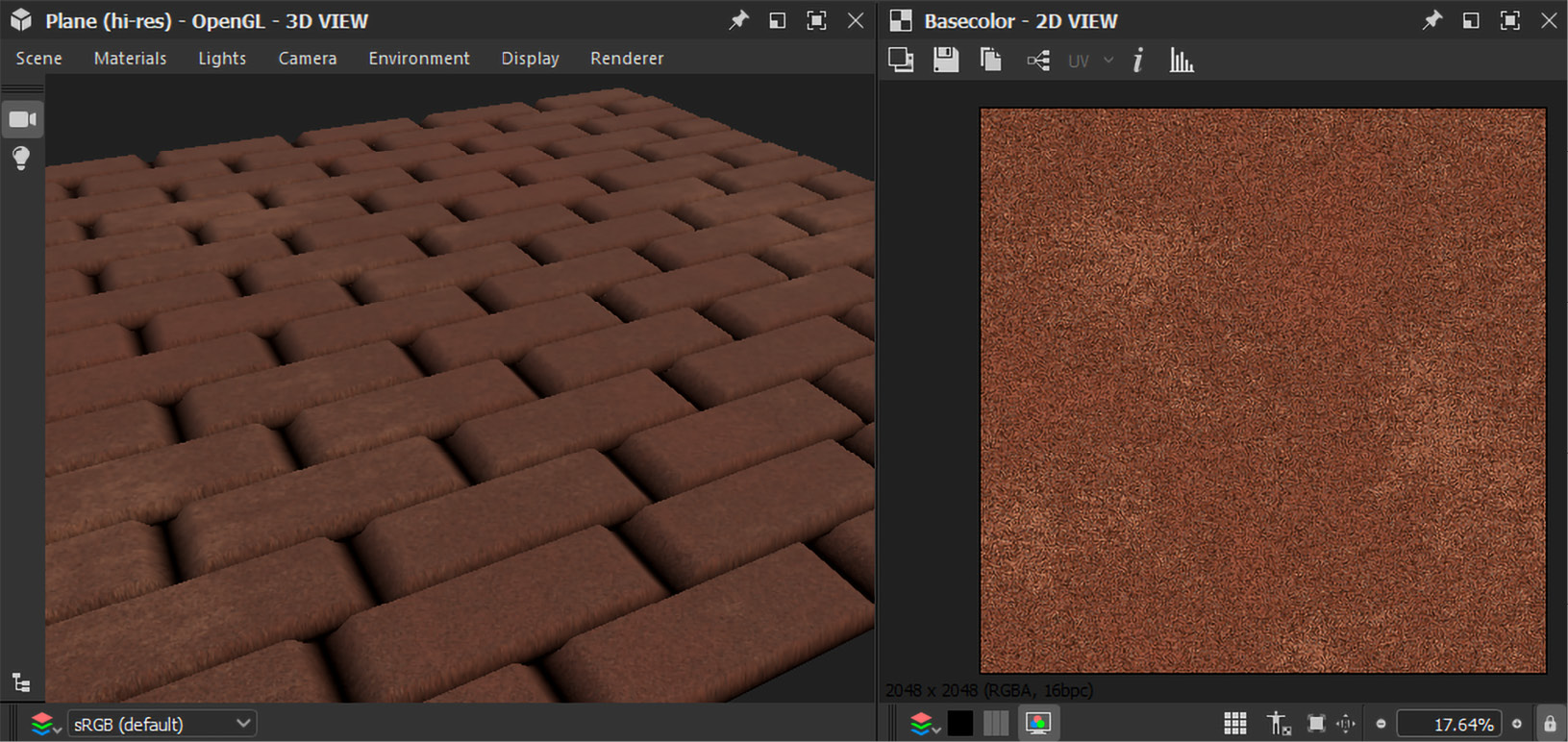
Figure 8.26 – Final output of the red brick tiles

I hope you have learned how the Tile Generator node works. Tile Generator has many other different parameters that appear in the PROPERTIES window. Similarly, there are many other parameters you can set for other different nodes, and studying them all in this book is not possible.

Nevertheless, these parameters are pretty much self-explanatory, which means you can easily learn by yourself – you just need to explore and experiment with them. In the following section, we will learn how to work with the Flood Fill node.

The Flood Fill node

Flood Fill is a part of a complex series of effects that enable you to greatly increase the diversity of a straightforward binary tile texture. It is not meant to be used on its own. Rather, it serves as a starting point for other Flood Fill effects. This segmented, separate data provides a more adaptable, effective, and harm-free method.

The Flood Fill node works with a secondary Flood Fill effect node, which includes Flood Fill to Gradient, Flood Fill to Color or Grayscale, Flood Fill to Random Color, Flood Fill to Random Grayscale, Flood Fill Mapper, Flood Fill to bbox size, Flood Fill to Position, Flood Fill Mapper, and Flood Fill to Index. However, we will only work on Flood Fill to Random Grayscale, Flood Fill to Position, and Flood Fill to Gradient, because these three are the most frequently used Flood Fill nodes.

The input map must be suitable for Flood Fill for it to function. An ideal binary map (black and white exclusively, no grayscale) would have a border around each tile that is completely black (0,0,0) for every pixel, separating it from the adjacent lines.

Tile Generator is one instance of software that is ideal for this. Problems occur when grayscale, sloping values are utilized – notably when tiles are not separated by whole black pixels.

This is discernible by a general lack of red values in the outcome and sometimes, by odd artifact lines. In these situations, either change the input map’s contrast or remove it. You test whether anything changes and make sure to adjust the Safety/Speed trade-off option.

1. Let’s try the Flood Fill to Random Grayscale node first. So, connect the Tile Generator node’s output to the Flood Fill node’s Mask input, and then connect the Flood Fill node’s Box output to the Flood Fill to Random Grayscale node’s Flood Fill input. Finally, connect the Flood Fill to Random Grayscale node’s output to the rest of the inputs, as shown in Figure 8.27:

Figure 8.27 – Flood Fill to Random Grayscale

2. Flood Fill to Random Grayscale will produce brick walls with random heights because all the heights of the bricks will become randomized, with variations of blacks and whites creating different height maps, normal maps, and AO, as shown in Figure 8.28:

Figure 8.28 – Flood Fill to Random Grayscale output result

3. Now, let us try Flood Fill to Position. So, replace Flood Fill to Random Grayscale with Flood Fill to Position. However, the Flood Fill to Position node’s output is colored. Therefore, we need to add the Grayscale Conversion node to any grayscale node – for example, we have to add the Grayscale Conversion node between the Flood Fill to Position node and the Normal map node, as shown in Figure 8.29:

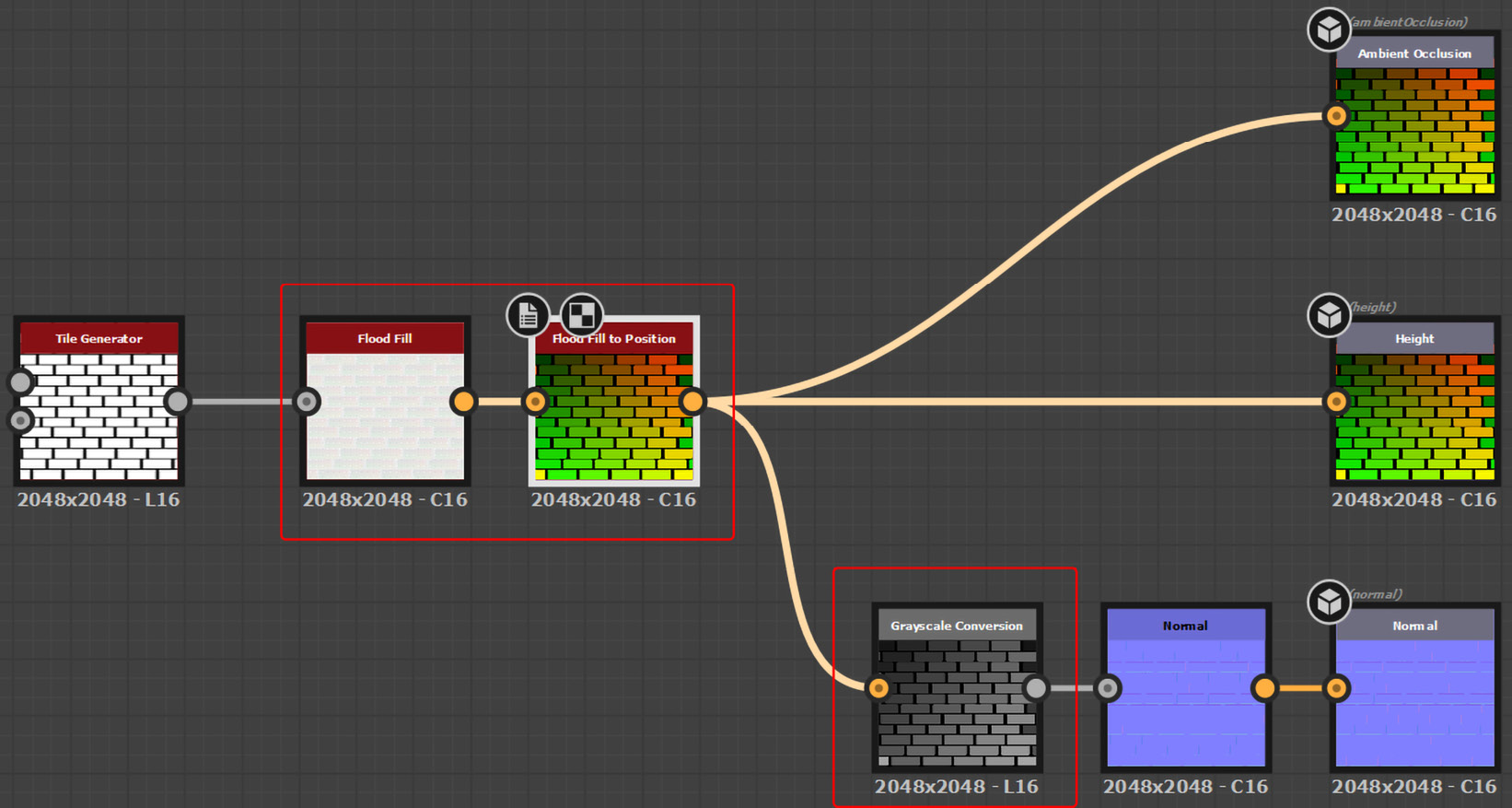
Figure 8.29 – Adding to the Flood Fill to Position node and the Grayscale Conversion node

4. The Flood Fill to Position node will create a gradient-like map, which will produce a stairs-like effect if applied to the height map. You can increase the material height if you want to see a more accurate result, as shown in Figure 8.30, and later, you can put it back to normal:

Figure 8.30 – The result of Flood Fill to Position

5. Let us replace Flood Fill to Position with Flood Fill to Gradient and remove the previously added Grayscale Conversion node because the Flood Fill to Position node creates a grayscale output:

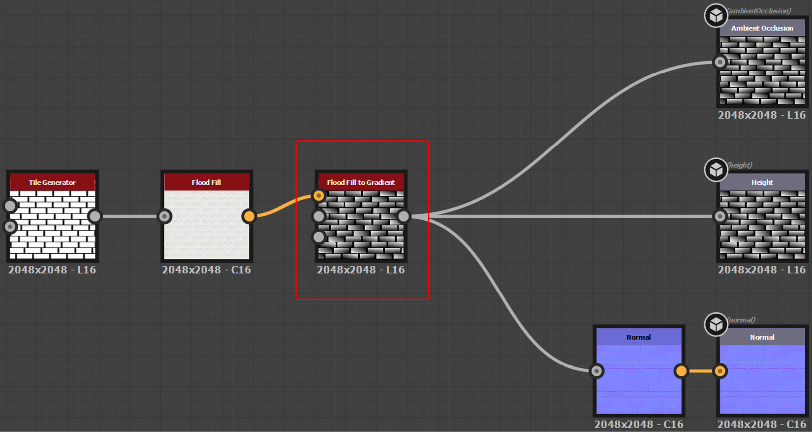
Figure 8.31 – Adding the Flood Fill to Gradient node

You will notice that the Flood Fill to Gradient node creates a gradient map on each brick rather than the whole brick wall.

6. The Flood Fill to Gradient node also has some useful parameters. Let us change one of the parameters, so double-click on the Flood Fill to Gradient node and increase Angle Variation up to 1.

This will randomize the direction of the gradient on each brick and it will look something like Figure 8.32. The Flood Fill to Gradient node is good for creating broken, eroded, or non-uniform textures.

7. You can also add your own variation by adding different noises to the Gradient node’s Angle Input and Slope Input settings and changing their parameters from the Flood Fill to Gradient node’s properties.

Figure 8.32 – The result of the Flood Fill to Gradient node

I hope these three useful Flood Fill effect nodes are now clear to you, and you have understood how to use them with the main Flood Fill node. In the next section will learn how the Quad Transform node works.

The Quad Transform node

The Quad Transform node allows you to distort the connected node either using the mouse or changing the parameters in the PROPERTIES window. Let us try to add a shape over the brick wall and distort it using the Quad Transform node and blend it using the Blend node:

1. In the GRAPH window, add the Star and Quad Transform Grayscale nodes – we will use the grayscale version of Quad Transform because the Star node is grayscale per se. Then, connect the Star node’s output to Quad Transform Grayscale node’s input, as shown in Figure 8.33:

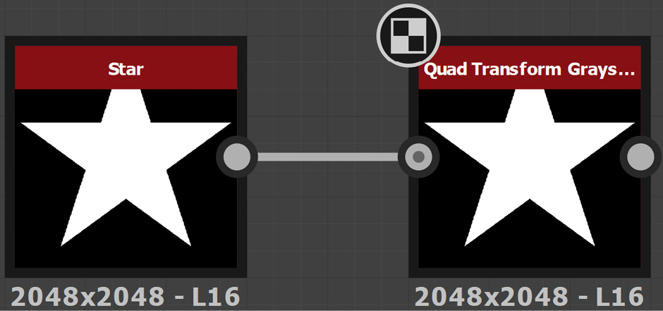
Figure 8.33 – Adding the Star and Quad Transform Grayscale nodes

2. Now, we have to blend the Star node using a secondary color with the brick wall. Therefore, add a Blend node and a different Uniform Color (as shown in Figure 8.34), so that we can blend the Star, existing Gradient Map color, and a different Uniform Color:

Figure 8.34 – Adding the Uniform Color and Blend nodes

3. Now, connect Uniform Color’s output to the Blend node’s foreground, connect Gradient Map’s output to the Blend node’s background, and Quad Transform Grayscale’s output to Blend node’s Opacity input. Then, connect the Blend node’s output to the Base Color node’s input. Your connection should look the same as in Figure 8.35:

Figure 8.35 – Connecting Uniform Color, Gradient Map, and Quad Transform Grayscale to Blend

4. Now, let us distort the Star shape node using the Quad Transform Grayscale node. Double-click on Quad Transform Grayscale with your mouse. The Star shape node shape will load in 2D VIEW with four corner points that you can move around with the mouse – or you can change its parameters under the p00, p01, p02, and p03 settings, as shown in Figure 8.36:

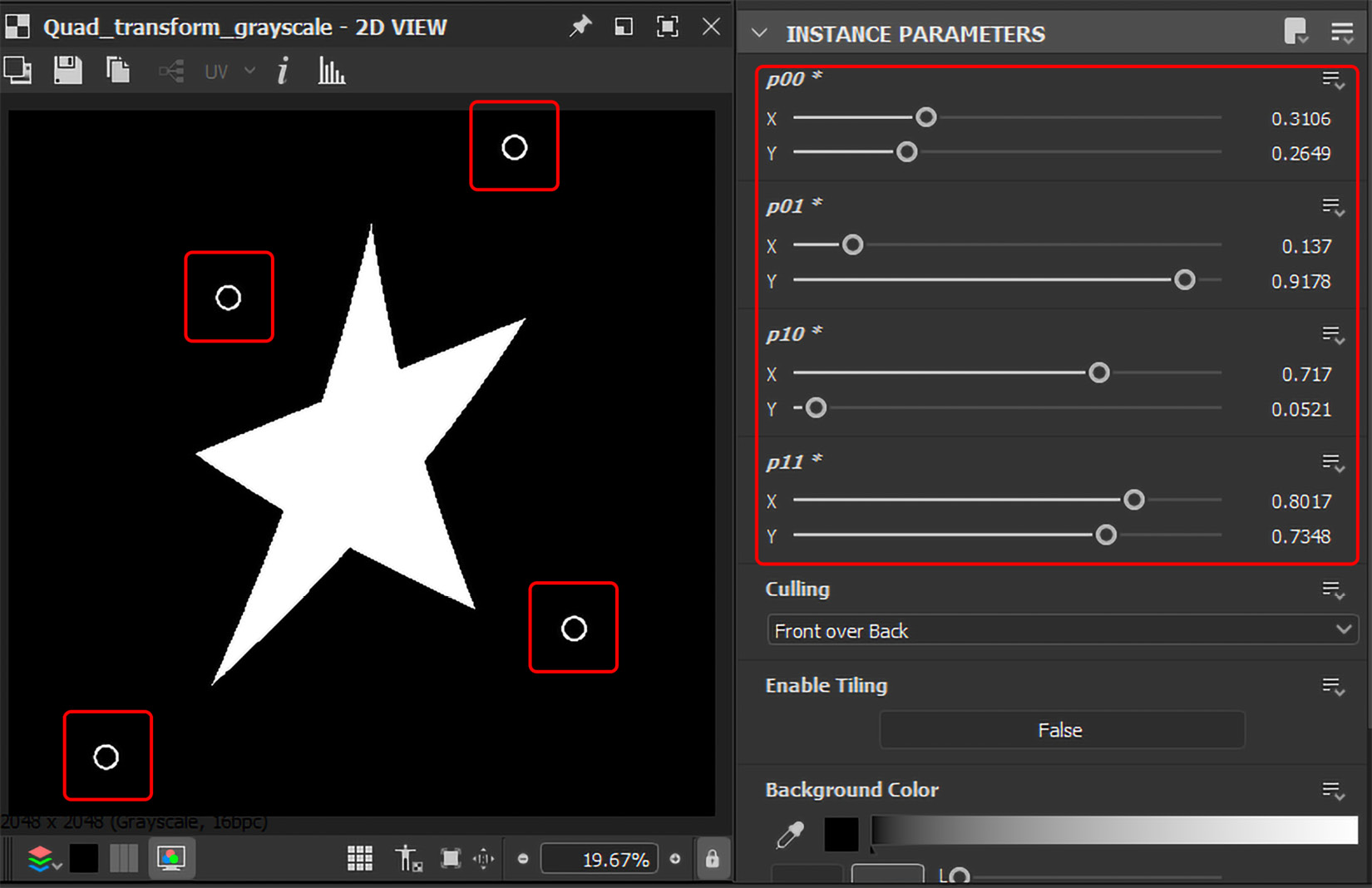
Figure 8.36 – Distorting the star-shaped node using the Quad Transform Grayscale node

5. The Quad Transform Grayscale node will distort the Star shape node and the Blend node will blend two nodes based on the mask. You can also double-click on Base Color with the mouse to produce the result, as shown in Figure 8.37.

If you don’t see the result in 3D VIEW, then right-click in the GRAPH window and choose View Outputs In 3D View:

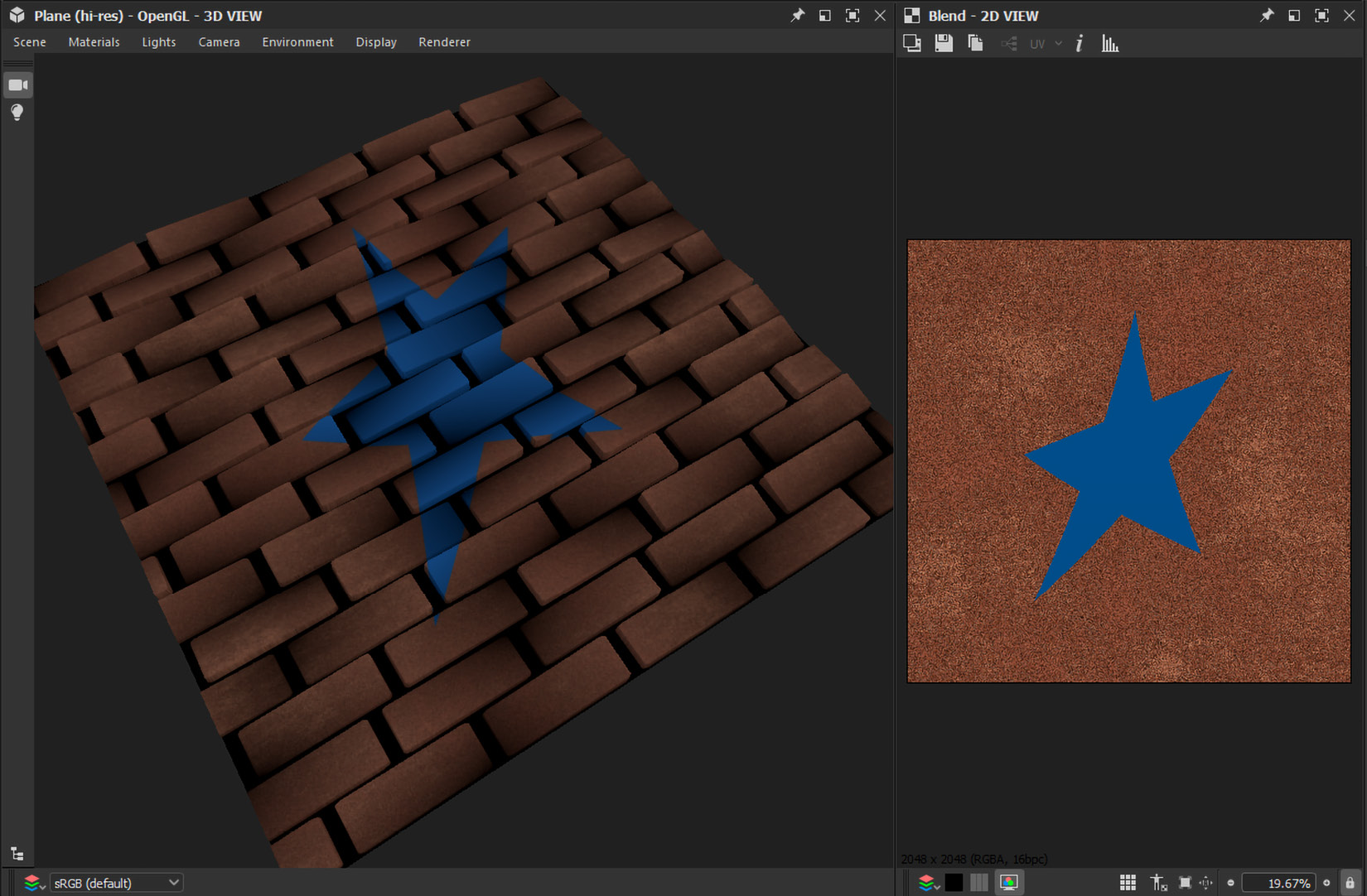
Figure 8.37 – The final result of the Quad Transform Grayscale and Blend nodes

I hope it’s clear now to you how to work with the Quad Transform node and the purpose of the Blend node. In the following section, we will learn about the Height Blend node.

The Height Blend node

The height data from the two combined height maps forms the foundation of the Height Blend node. It produces a blended height map as well as a black and white mask that may be used everywhere.

So, let us make two height maps and combine them using the Height Blend node.

1. Select the existing Flood Fill to Gradient node and using the keyboard, press Ctrl + C (on Windows) or Command + C (on Mac), and then press Ctrl + V (on Windows) or Command + V (on Mac) to copy and paste it. You can also use Ctrl + D (on Windows) or Command + D (on Mac) to duplicate the nodes instead of copying and pasting them. Then, change the Angle Variation setting of the copied Flood Fill to Gradient node to 0.5:

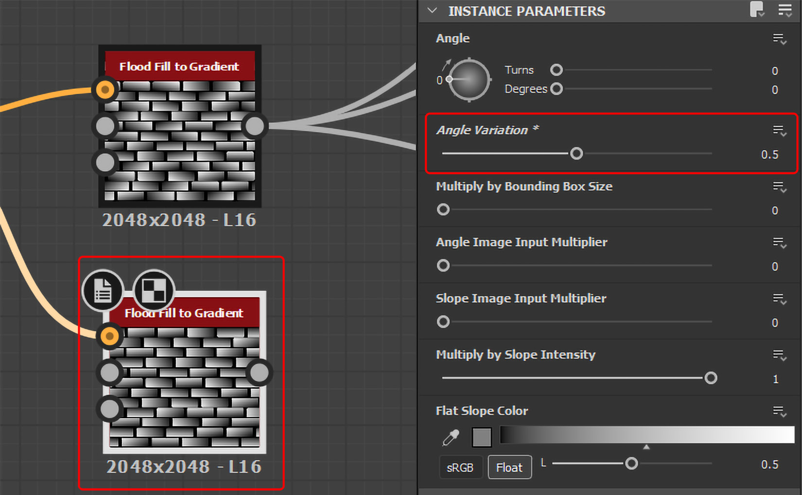
Figure 8.38 – Copying and pasting Flood Fill to Gradient and changing its angle variation

2. Now, add the Height Blend node to the GRAPH window and connect the original Flood Fill to Gradient’s output to the Height Blend node’s Height Top and the copied Flood Fill to Gradient’s output to the Height Blend node’s Height Bottom and connect the Height Blend node’s Blended Height to the inputs of the Ambient Occlusion, Height, and Normal nodes, as shown in Figure 8.39:

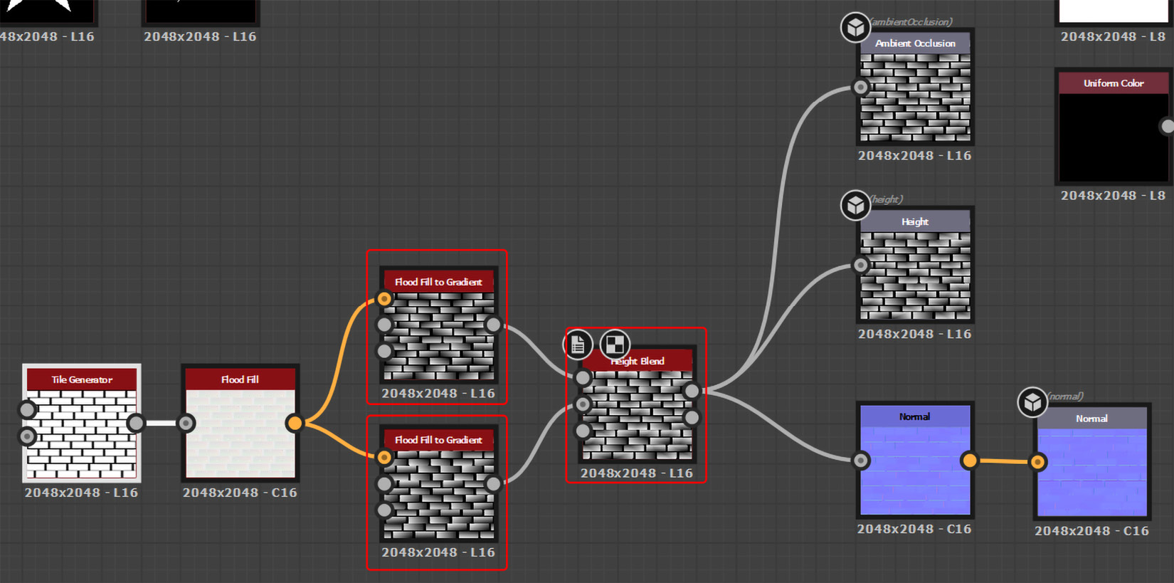
Figure 8.39 – Adding the Height Blend node

3. The Height Blend node will combine the gradients of the original and copied Flood Fill to Gradient nodes and will produce an interesting result, as shown in Figure 8.40:

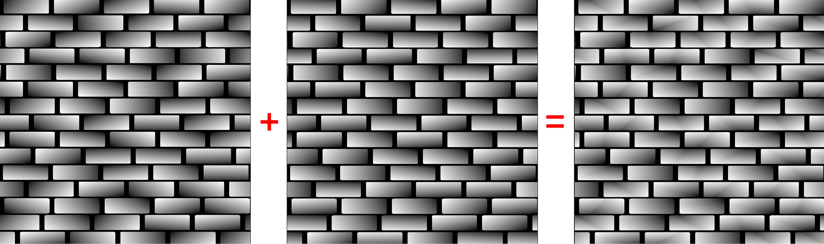
Figure 8.40 – The result of the Height Blend node

4. If you want, you can change the parameters of the Height Blend node to get the desired result. If you don’t see the result in 3D VIEW, then right-click in the GRAPH window and choose View Outputs In 3D View:

Figure 8.41 – The final output of the Height Blend node

It is used to blend two height maps based on a mask. Additionally, it generates a mask and has controls for the contrast, because you can use it to blend all kinds of height maps. In the following section, we will learn about the Curve node.

The Curve node

The Curve node provides a picture tone remapping interface, similar to other 2D image-altering tools. The user can remap the input, which can be either monochrome or colored, by setting points and modifying Bezier curves. It is extremely helpful when used to remap gradient transitions to a particular height profile.

This enables incredibly accurate modeling of bevel profiles and other similar shapes. The Curve node provides a full-featured curve editor instead of the conventional basic UI with sliders and settings that most other nodes have.

So, let us apply Curve to some existing nodes:

1. In Figure 8.42, you will notice that the Tile Generator brick map is blurry at the edges. We need to remove this blurriness:

Figure 8.42 – Tile Generator blurry edges

2. Add the Curve node between Tile Generator and Flood Fill, as shown in Figure 8.43, and then double-click Curve to activate its parameters inside the PROPERTIES window.
3. Once you see the diagonal curve graph, double-click in the middle of the line, as shown in Figure 8.43, to add a Curve point. This will also add points at both ends of the curve:

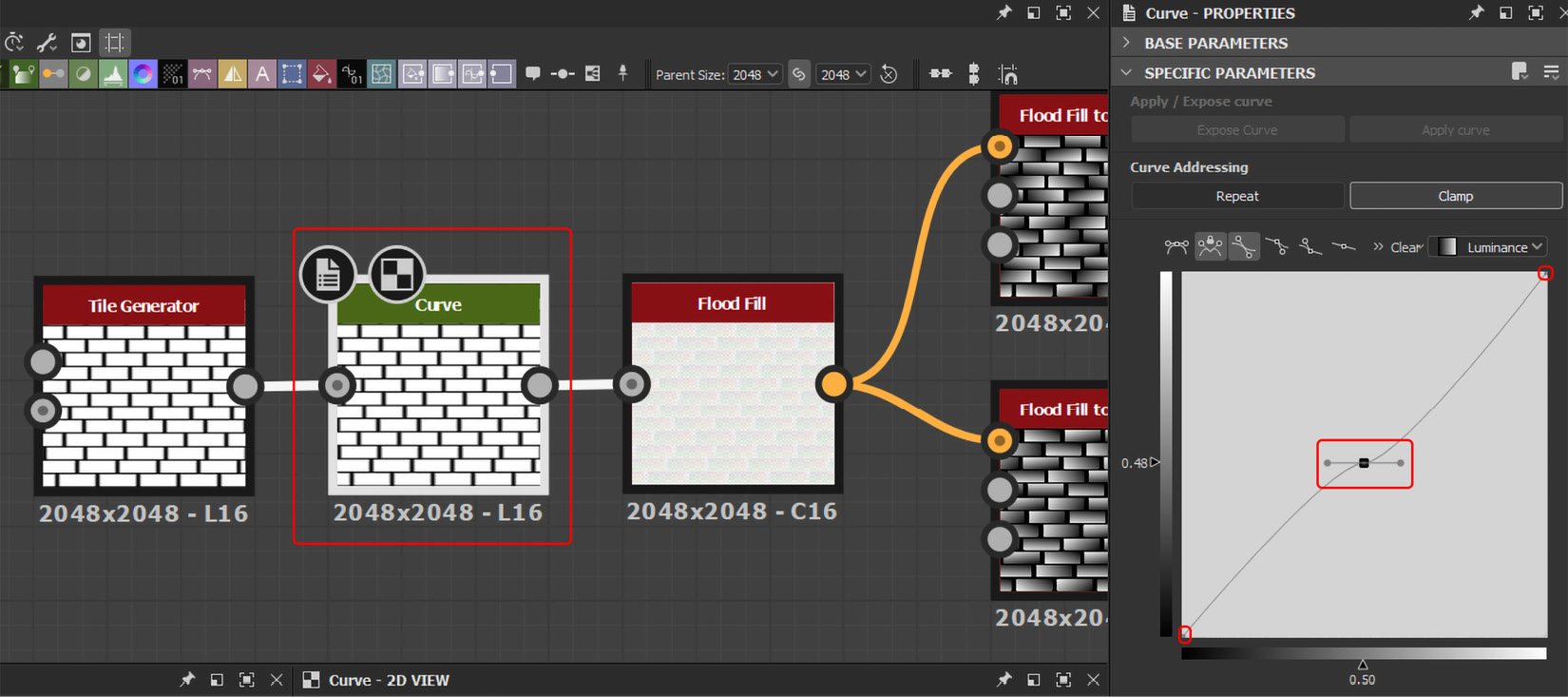
Figure 8.43 – Adding points to the curve

Now, we only need the points at both ends of the curve. Therefore, we will delete the middle point because we only added it to activate the endpoints.

4. After deleting the middle point, move the endpoint at the bottom left all the way to the right, which will make the Tile Generator bricks sharp and clear, as shown in Figure 8.44:

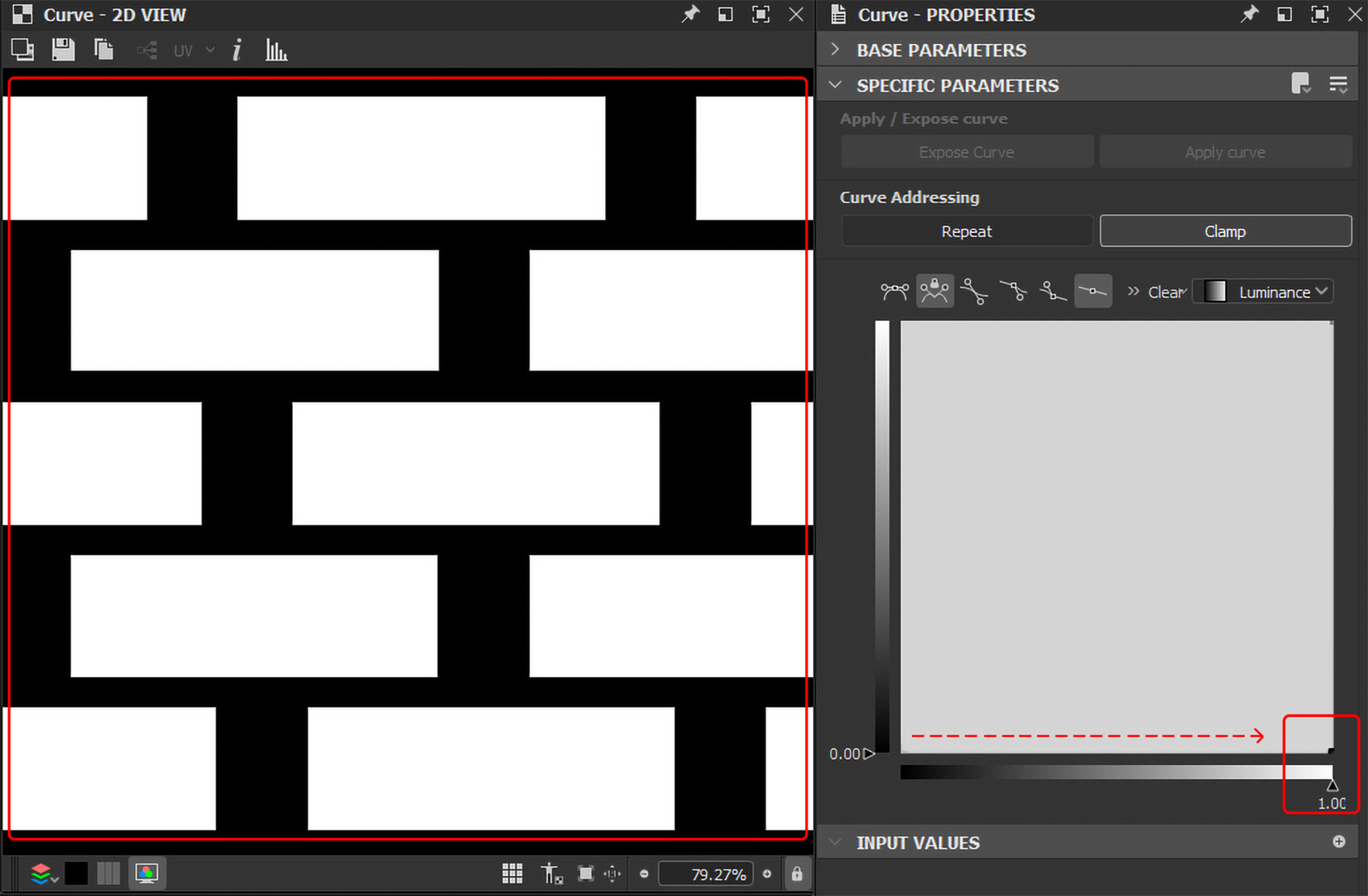
Figure 8.44 – Moving the bottom left endpoint to the right

You will now notice that the Tile Generator bricks now have more gaps between them.

5. Left-click on Tile Generator (don’t double click – otherwise, 2D View will change to Tile Generator) and change Pattern Specific to 0.03, as shown in Figure 8.45:

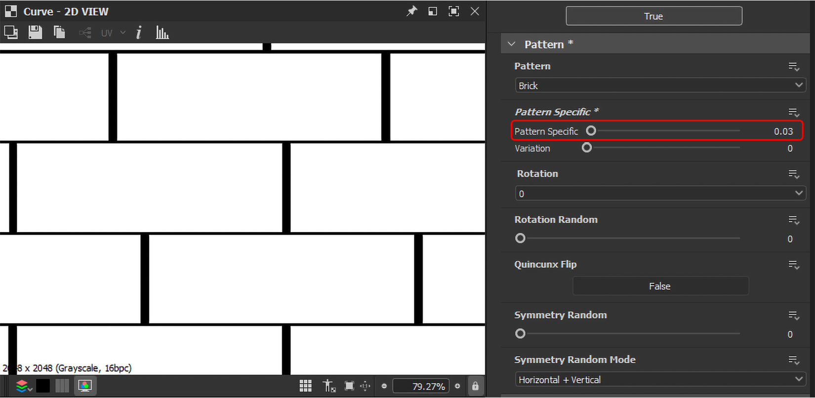
Figure 8.45 – Changing the Pattern Specific value of Tile Generator

You can also add more points to the Curve node – move the Beziers around it and reshape the curve as required. I hope the purpose of this node is clear to you. We will work on the Curve node more in Chapter 10, Creating Television Shelf in Adobe Substance 3D Designer. In the following section, we will add some Dirt and Dust to the existing brick wall.

The Dirt and Dust nodes

The Dirt and Dust nodes work with inputs from the Ambient Occlusion, Curvature, Position, World Space Normal, and Mask (optional) nodes.

The Dirt node produces a dirt map effect using all the aforementioned nodes, while the Dust node produces a dust map effect using only Ambient Occlusion, World Space Normal, and Mask (optional).

So, let us apply the Dirt and Dust effects to our project:

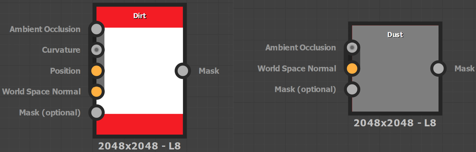
Figure 8.46 – The Dirt and Dust nodes

The Ambient Occlusion node that we have is merely an Output node as shown in Figure 8.47:

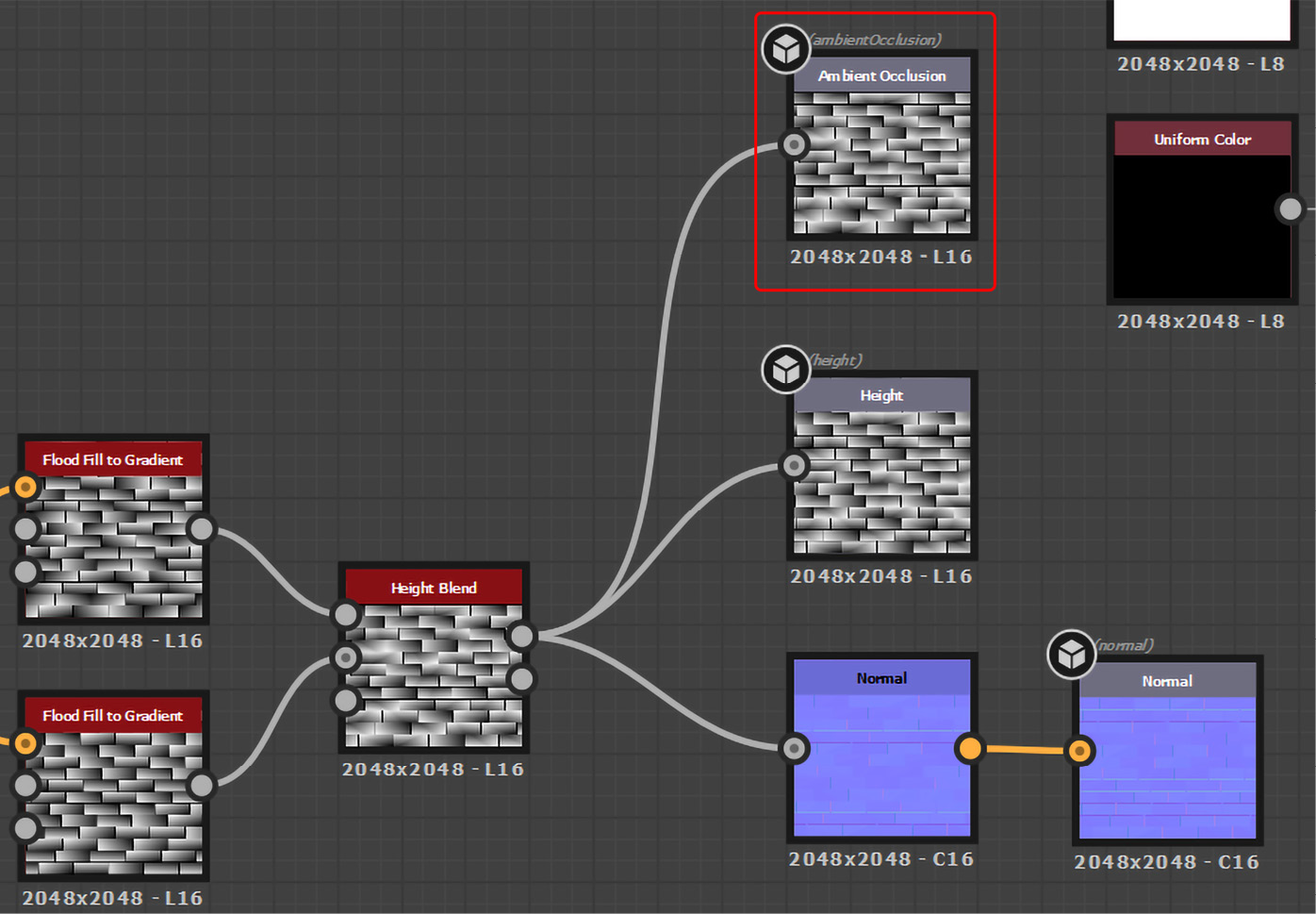
Figure 8.47 – A single Ambient Occlusion input node

Therefore, we need to add Ambient Occlusion (HBAO) between the Height Blend and Ambient Occlusion inputs, as shown in Figure 8.48.

You can study more about Ambient Occlusion (HBAO) and Ambient Occlusion (HTAO) in the Atomic nodes section.

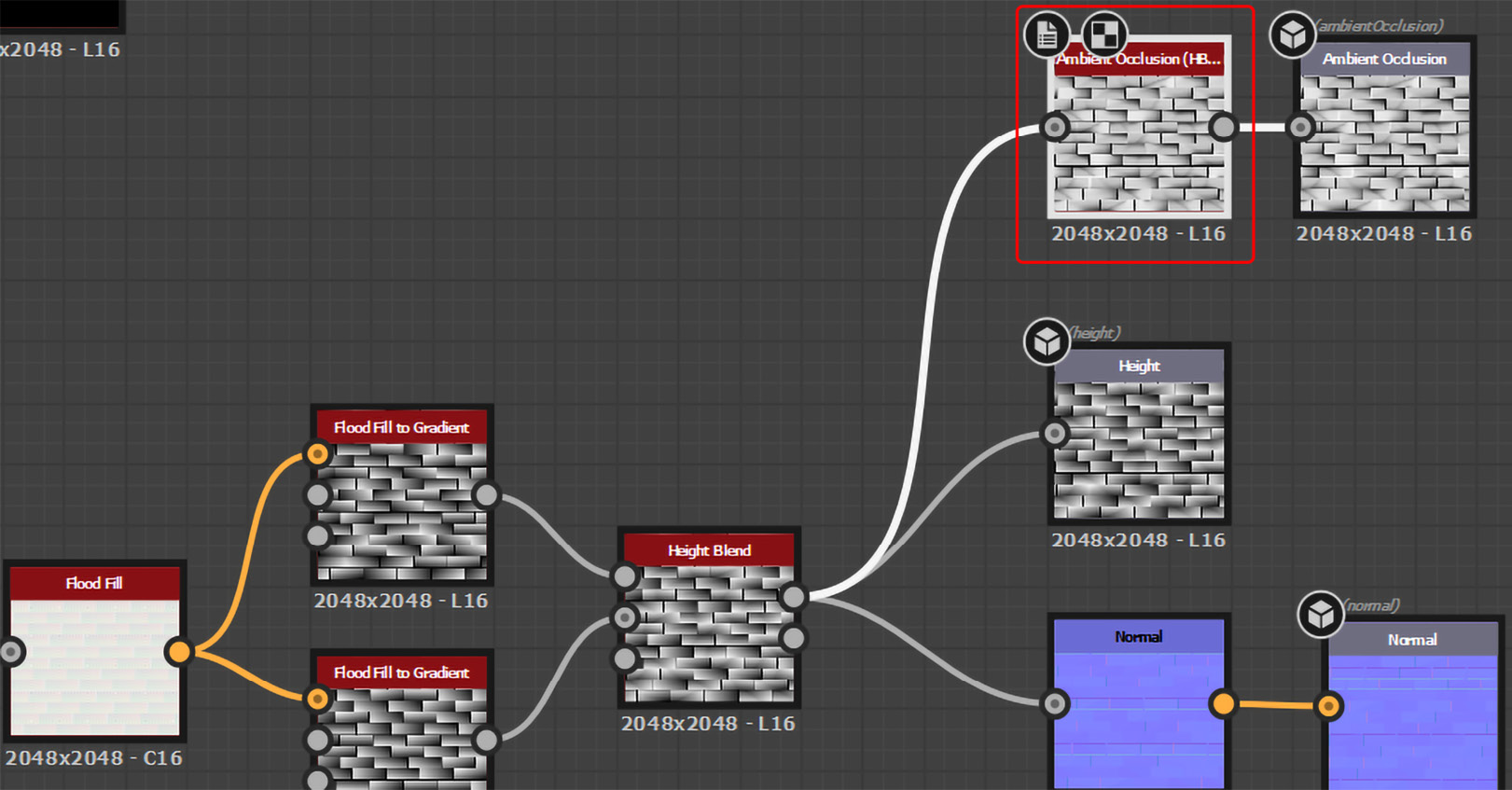
Figure 8.48 – Adding Ambient Occlusion (HBAO)

6. Now, add the Curvature Smooth node and connect the Normal map node’s output to the Curvature Smooth node’s Normal input, as shown in Figure 8.49:

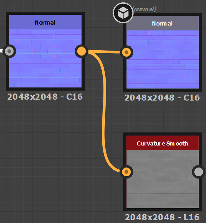
Figure 8.49 – Adding the Curvature Smooth node

7. Once all the nodes are ready, it is time to connect them. Therefore, connect Ambient Occlusion (HBAO) to the Dirt node’s Ambient Occlusion input, Curvature Smooth to the Dirt node’s Curvature input, and Normal to the Dirt node’s World Space Normal input, as shown in Figure 8.50:

Figure 8.50 – Adding nodes to the Dirt node’s inputs

8. Now, we need to blend our Dirt map with the dirty-looking color. Therefore, add a dark brownish Uniform Color node and a Blend node, and connect the dark brownish Uniform Color node’s output to the newly created Blend node’s Foreground input and the Dirt node’s Mask output to the newly created Blend node’s Opacity input, as shown in Figure 8.51:

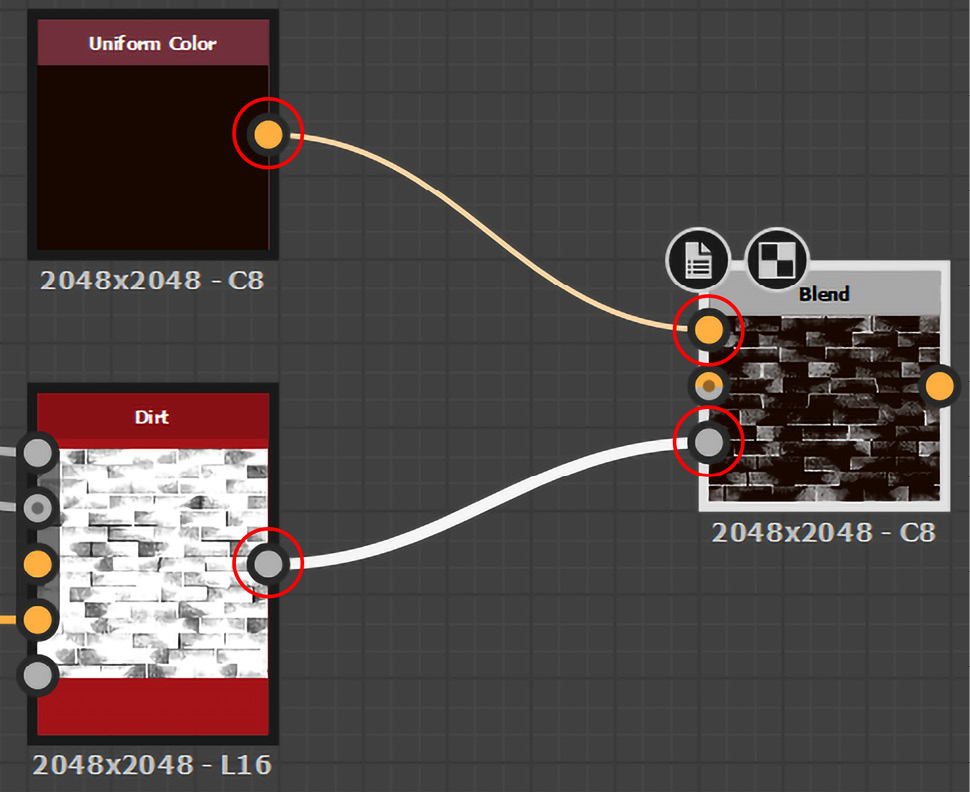
Figure 8.51 – Connecting the Uniform Color and Dirt nodes to the Blend node

At this point, we don’t need our previously created Base Color node. Hence, we need to disconnect it from its Blend node in order to create a new Base Color node with the Dirt effect. However, you should only disconnect it and not delete it:

Figure 8.52 – Disconnecting the Base Color node

9. Now, move all the Base Color-related nodes to the bottom of the Height Blend-related nodes. Connect the old Blend node’s output to the newly created Blend node’s Background input and the newly created Blend node’s output to the Base Color node’s input:

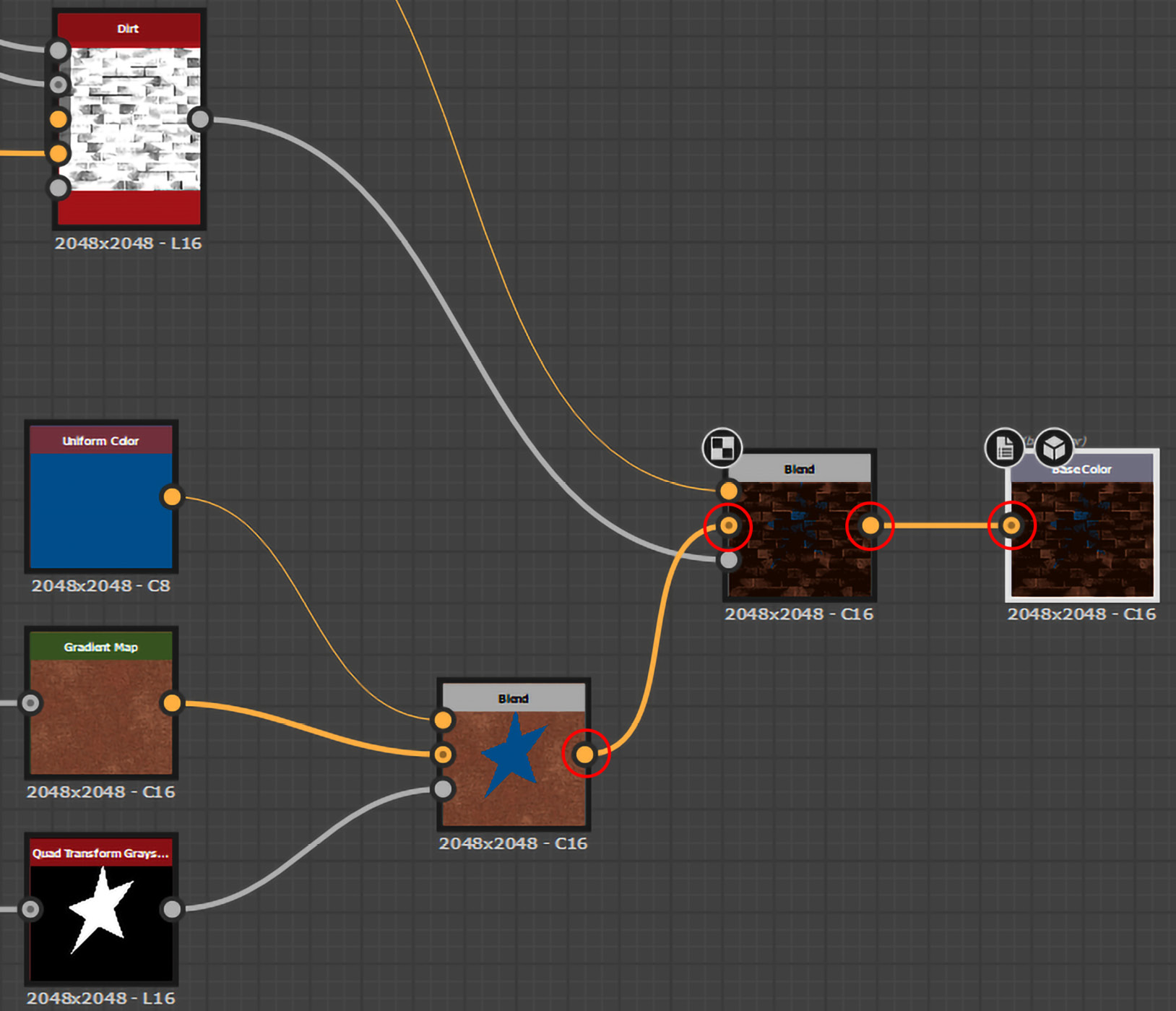
Figure 8.53 – Connecting the old and new Blend nodes to Base Color

10. Double-click the Dirt node and change the following settings under INSTANCE PARAMETERS (which are specifically related to the selected node):
    • Dirt Level: 0.7, Dirt Contrast: 0.2, Grunge Amount: 0.4
    • Edges Masking: 0.3, Grunge Scale: 1

These parameters will produce a realistic Dirt effect on the brick wall, as shown in Figure 8.54.

Figure 8.54 – The Dirt node effect

11. Similarly, you can add the Dust node, and connect the existing Ambient Occlusion (HBAO) node’s output to the Dust node’s Ambient Occlusion input, and the Normal map node’s output to the Dust node’s World Space Normal input:

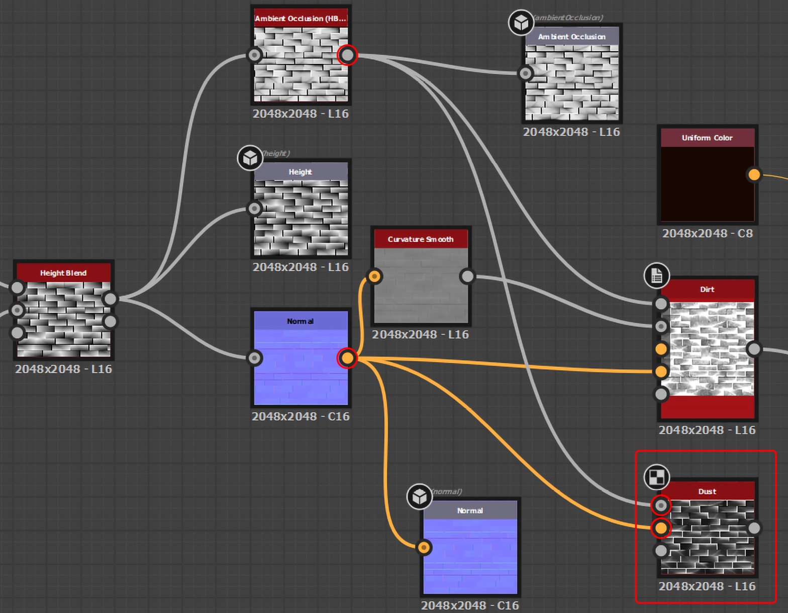
Figure 8.55 – Adding the Dust node

12. Now, add a new Blend node for the Dust effect. We will name this Blend node Dust Blend and the older one Dirt Blend to avoid confusion.
13. Add a new Uniform Color node that resembles sand. Then, connect the sandy Uniform Color output to the Dust Blend node’s Foreground input, and the Dust node’s Mask output to the Dust Blend node’s Opacity input, as shown in Figure 8.56:

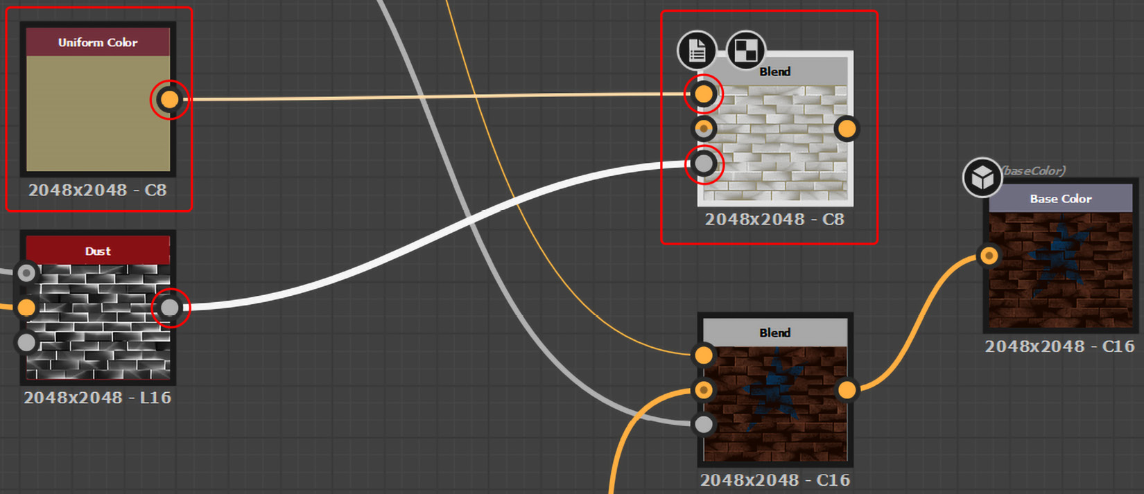
Figure 8.56 – Connecting the new sandy Uniform Color node and the Dust node to the new Blend node

14. Disconnect the Dirt Blend node and the Base Color node in order to create a new node system. Now, connect the Dirt Blend node’s output to the Dust Blend node’s Background input and connect the Dust Blend node’s output to the Base Color node’s input, as shown in Figure 8.57:

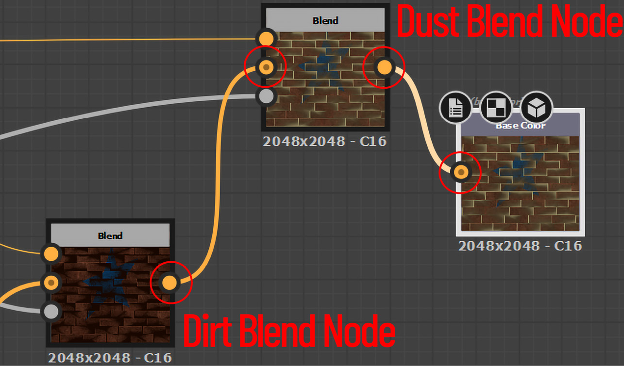
Figure 8.57 – Adding the Dust effect to Base Color

15. You will now notice a visible dust effect on the brick wall. If you want, you can also change the INSTANCE PARAMETERS settings of the Dust node:

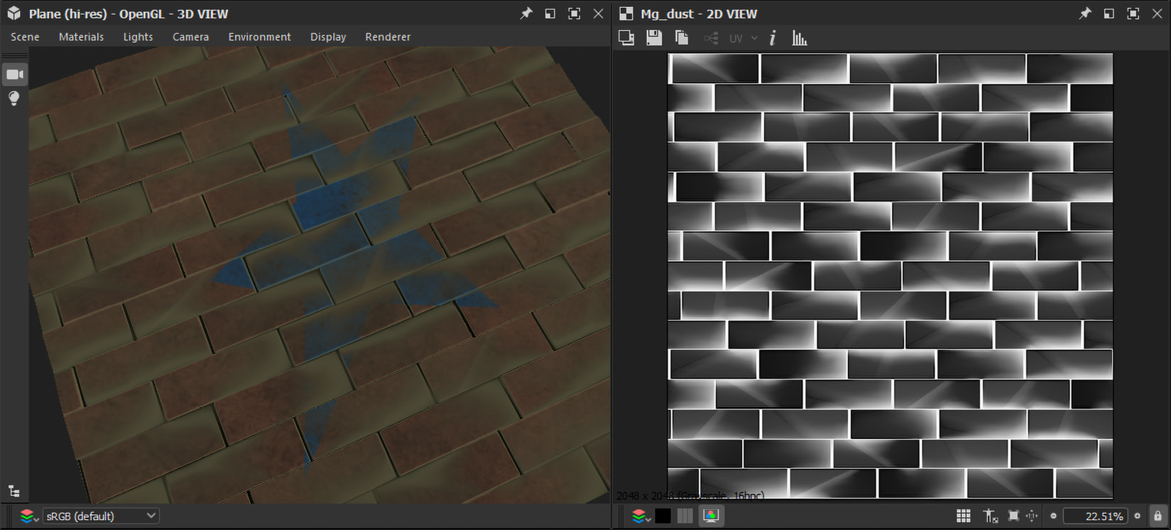
Figure 8.58 – The Dust node’s final output

You can also use the dirt effect or the dust effect by themselves. However, we blended both of these nodes so that you could also learn more about the Blend node. In the following section, we will learn about the Shape Mapper node.

The Shape Mapper node

With the help of the Shape Mapper node, you can control and modify any existing Shape node, Star node, or other similar nodes. The Shape Mapper node manipulates your existing shape into a Circle or Polygon form using other INSTANCE PARAMETERS settings.

Let us do some experiments on our existing Star node:

1. Add the Shape Mapper node in the GRAPH window, and then connect the Quad Transform Grayscale node’s output to the Shape Mapper node’s input and the Shape Mapper node’s output to the Blend node’s Opacity input, as shown in Figure 8.59:

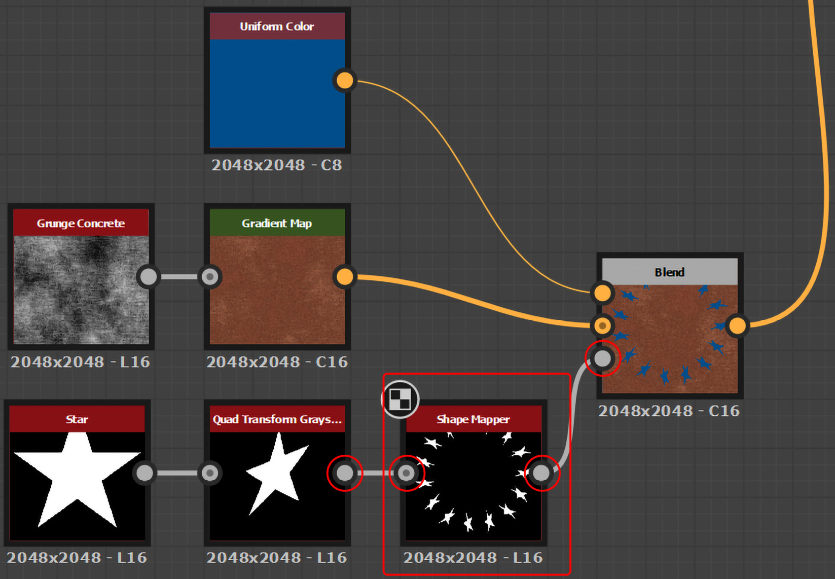
Figure 8.59 – Adding the Shape Mapper node

2. The final output of the Shape Mapper node will look similar to Figure 8.60. However, you can change the Shape Mapper node’s INSTANCE PARAMETERS settings if you want a different result:

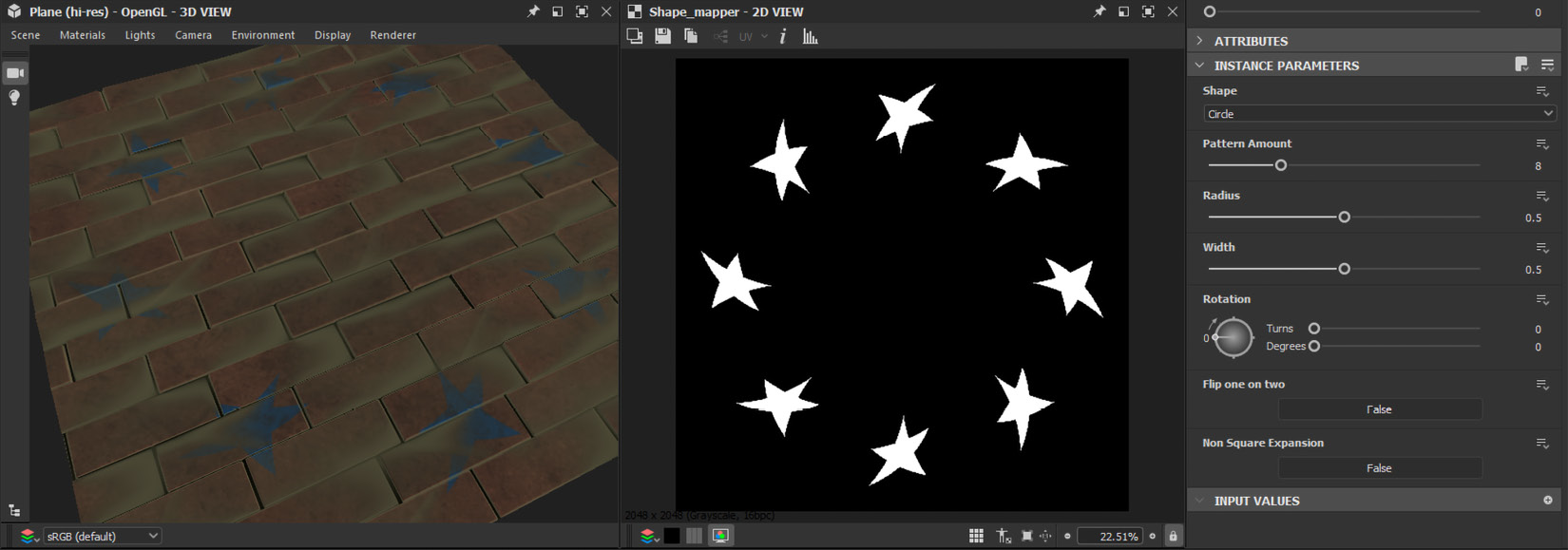
Figure 8.60 – The Shape Mapper node’s final output

I hope it is now clear to you the purpose of the Shape Mapper node and how it works. In the following section, we will learn about how we can work with the Shape Splatter node.

The Shape Splatter node

This is an extremely complicated node that should be utilized with Shape Splatter Data Extract, Shape Splatter to Mask, and Shape Splatter Blend. Nevertheless, it is optional to use these conjunction nodes.

It is similar to Tile Sampler or Tile Generator in that it is used to produce shapes, but it uses a dynamic, non-destructive method that gives the user control over each stage through a multi-level system.

Shape Splatter is a more sophisticated variant of Flood Fill, which creates the map and associated data in a single phase, as opposed to Flood Fill, which requires a basic input map from an external source.

However, don’t worry, I will make it easier for you to comprehend this node. We need to start by opening a new Metallic Roughness substance graph.

1. Create a new Metallic Roughness substance graph and name it Shape Splatter Test.
2. Go to 3D VIEW and choose Plane (hi-res) from the Scene menu. Then, click on the Material menu, select the Default menu, and choose Tesselation + Displacement from the Metallic Roughness menu.
3. Once the Height parameter has loaded, change Scale to 5 and Tessellation Factor to 16:

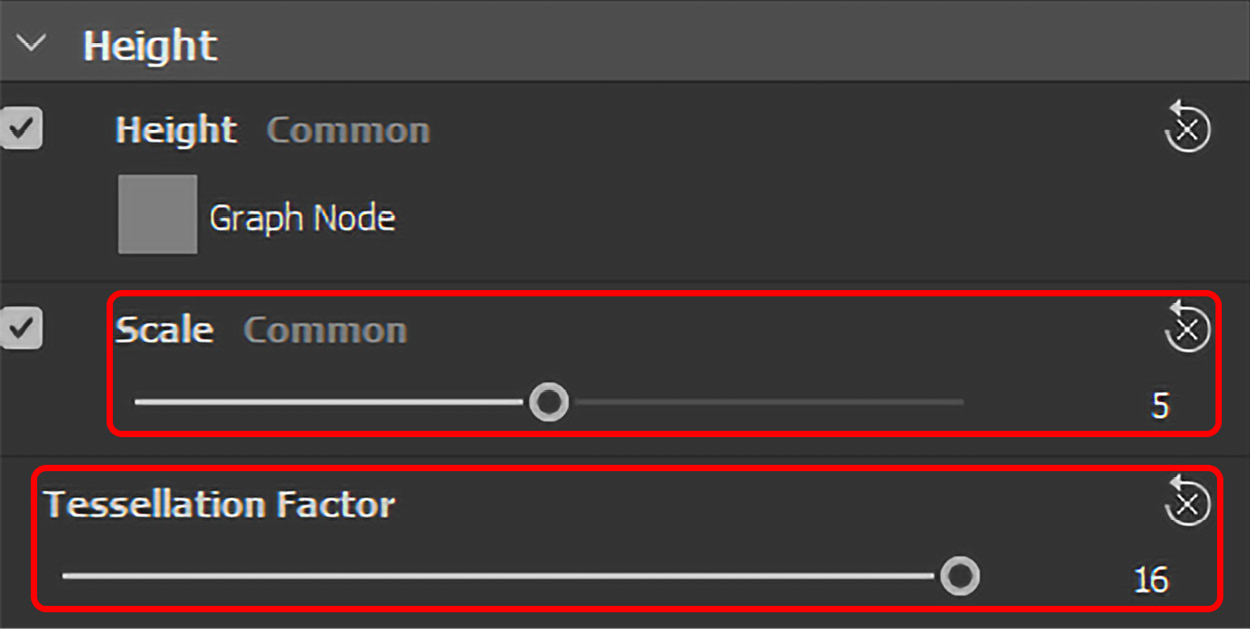
Figure 8.61 – Adjusting the material height settings from the PROPERTIES window

4. Now, add the Shape Splatter node into the GRAPH window. However, we need a Background Height node and two Pattern nodes to connect to the Shape Splatter node. Therefore, we will add a Perlin Noise node, a Shape node, and a Star node, as shown in Figure 8.62:

Figure 8.62 – The Shape Splatter, Perlin Noise, Shape, and Star nodes

5. We need to change the shape inside the Shape node, so double-click the Shape node, and from the PROPERTIES window, change Pattern to Disc and Scale to 0.7 under the INSTANCE PARAMETERS settings:

Figure 8.63 – Adjusting the Shape node

6. Now, connect Perlin Noise to the Shape Splatter node’s Background Height. Then, we have to connect the Shape and Star nodes to two Pattern nodes. However, we only have one – therefore, double-click the Shape Splatter node, and under the INSTANCE PARAMETERS settings, change Pattern Input Number to 2, and then connect the Shape node to the Shape Splatter node’s Pattern 1 input and the Star node to the Pattern 2 input, as shown in Figure 8.64:

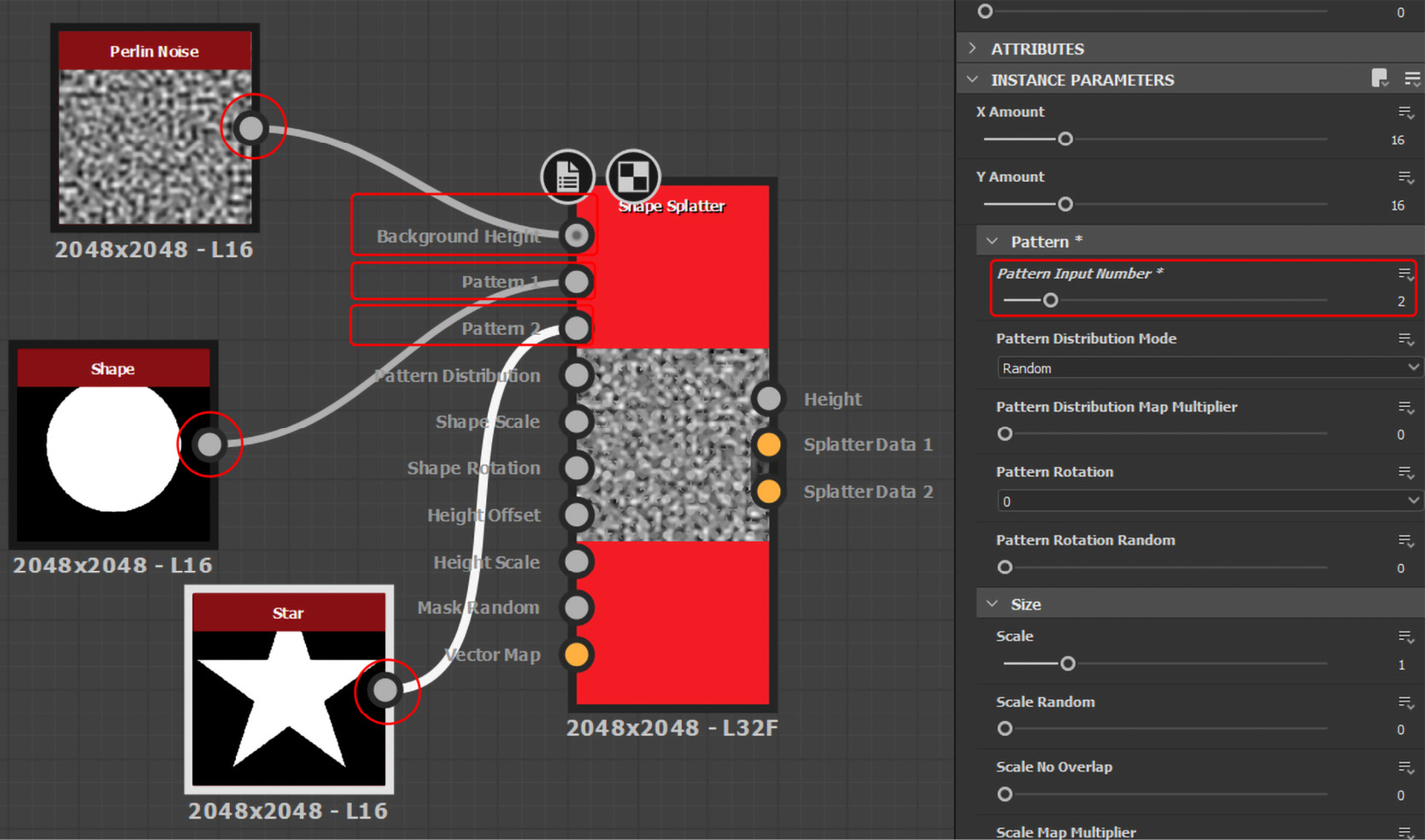
Figure 8.64 – Connecting the nodes to Shape Splatter

7. Now, connect the Shape Splatter node’s Height output to the Normal map node, the Height map node, and the Ambient Occlusion node via Ambient Occlusion (HBAO), as shown in Figure 8.65:

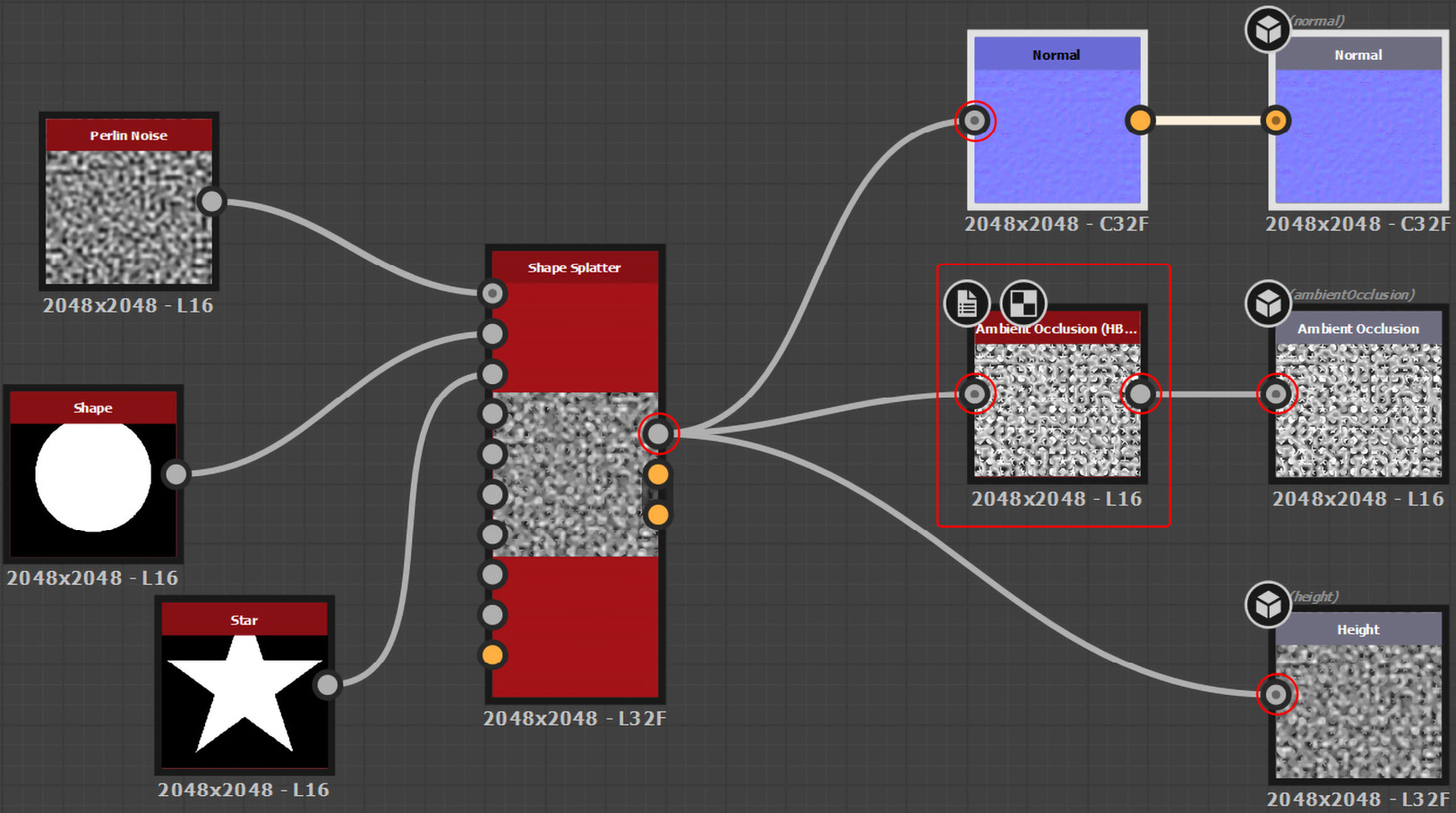
Figure 8.65 – Connecting the Shape Splatter node to Normal, Height, and Ambient Occlusion

8. Double-click on the Perlin Noise node and change its Scale to 12 under INSTANCE PARAMETERS in the PROPERTIES window.
9. Now, double-click on the Shape Splatter node to change the following parameters in the PROPERTIES window:
   • INSTANCE PARAMETERS: X Amount = 8, Y Amount = 8 (to reduce the number of patterns)
   • Size: Scale = 0.6 (to reduce the overall size of the patterns)
   • Position: Position Random = 0.5 (to randomly place the patterns)
   • Rotation: Rotation Random = 0.17 (to randomize the rotation angle of each pattern)
   • Height: Height Offset = 1 (to increase the height distance of patterns)
   • Height: Height Scale = 0.97 (to increase the height of displacement)
   • Height: Conform to Background = 1 (this will allow all the patterns to conform with Background Height and follow its height peaks)

Figure 8.66 – Applying the changes to the Shape Splatter parameters

Let us add some color to the Shape Splatter node using the Shape Splatter Blend Color node.

10. Add the Shape Splatter Blend Color node and increase its Pattern input to 2, and connect three different Uniform Color nodes to the Shape Splatter Blend Color node’s Background, Pattern 1, and Pattern 2 inputs.
11. Then, connect the Shape Splatter node’s Splatter Data 1 and Splatter Data 2 outputs to the Shape Splatter Blend Color node’s Splatter Data 1 and Splatter Data 2 inputs, and connect the Shape Splatter Blend Color node’s output to the Base Color’s input, as shown in Figure 8.67:

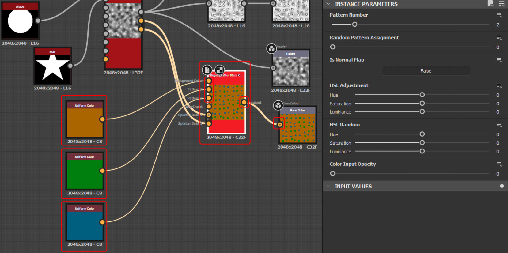
Figure 8.67 – Connecting the Shape Splatter node to the Shape Splatter Blend Color node

The Shape Splatter and Shape Splatter Blend Color nodes will produce a combination of different patterns conforming to the height peaks of the background in different colors, as shown in Figure 8.68:

Figure 8.68 – The final result of the Shape Splatter node and the Shape Splatter Blend Color node

Hopefully, you got the idea behind the Shape Splatter node. You can use this node in combination with the Shape Splatter Blend Color node and create interesting effects, such as adjusting the Height map of coins on the ground or the Base Color of stickers placed on the wall. In the following section, we will learn about the Histogram Scan node.

Histogram Scan

Histogram Scan is a node that offers an easy way to remap the contrast and brightness of input grayscale maps. This node is very basic yet helpful and can be used to dynamically grow and shrink masks.

So, let us work with this node:

1. In Figure 8.68, you will notice that the Perlin Noise node’s height is quite smooth – what if we need Perlin Noise to have flat height peaks like the Grand Canyon? This is where Histogram Scan comes in handy. Therefore, add the Histogram Scan node into the GRAPH window.
2. Connect the Perlin Noise node’s output to the Histogram Scan node’s input and connect the Histogram Scan node’s output to the Shape Splatter node’s Background Height input.
3. Then, change the Histogram Scan node’s Position parameter to 0.43 and the Contrast parameter to 0.69 in the PROPERTIES window under the INSTANCE PARAMETERS settings, as shown in Figure 8.69:

Figure 8.69 – The final output of the Histogram Scan node

I hope the Histogram Scan node’s purpose is clear to you. With this node, you can easily turn fuzzy and blurry shapes sharper, and this node can be also used instead of the Curve node.

Summary

As we are finally done with this chapter, I hope you comprehended all the topics and gained the skills to work with the nodes explained in this chapter. With the knowledge and expertise, you have gained in this chapter, you can now create materials such as brick walls, cracked walls, chipped paint, and other damage effects.

In the next chapter, you will get a chance to explore the Blending Modes in Adobe Substance 3D Designer. This feature is crucial owing to its ability to blend different nodes using procedural method to create interesting results. Every blending mode in the next chapter will be explained in detail, so get ready for it!