
5
Models for Claim Counts
Models and statistics for the number of claims can be built on counts in either discrete or continuous time. In practice, actuaries often look at the aggregate number of claims that have occurred within a fixed time interval (e.g., one calendar year) rather than studying the full stochastic process developing over time.
Whereas in real‐life applications one only obtains information in discrete time, for instance with information about the date of the claim events, continuous time modelling can be a more flexible and tractable tool that also allows the implementation of stylized features (such as lack of memory) in a transparent and elegant way. From the continuous time stochastic process approach one can then go back to implications for the discrete time intervals. For this reason, in this chapter we start with the general mathematical treatment of claim number modelling in continuous time. Section 5.4 will then treat the discrete case, and Section 5.5 deals with statistical procedures to fit such counting models to data for both approaches. Finally, in Section 5.6.1 we will discuss how to move from models for a number of claims for the insurer to the ones for the reinsurer.
Assume that claims happen at specific time points {T1, T2, …, Tn, …} that form an increasing sequence of necessarily dependent random variables. The claim counting process {N(t), t ≥ 0} can then be defined in terms of the claim instants by
5.1 General Treatment
A stochastic process N = {N(t);t ≥ 0} that counts the number of claims up to time t has to be a counting process. This means that we require the process to satisfy the following four and evident conditions:
- N(t) ≥ 0
- N(t) is integer valued
- If s < t, then N(s) ≤ N(t)
- for s < t, N(t) − N(s) equals the number of claims that have occurred in the time interval (s, t].
We note that the sample paths of a counting process are non‐decreasing and right‐continuous. In many cases one assumes that the jumps are only of size one so that multiple claims at the same time instance are excluded.
5.1.1 Main Properties of the Claim Number Process
The distribution of N(t), the number of claims up to time t, can be given in explicit form
It can also be introduced via the (probability) generating function

which is at least defined for |z| ≤ 1, but often the radious of convergence is larger. Apart from the expression pn(t) we will introduce a (c.d.f) of N(t), that is, the probability of at most r claims up to time t:

Among the main characteristics of a claim number process we should mention a variety of possible moments and derived quantities. The function Qt(z) can be used to evaluate these consecutive moments of N(t). Here are a few of the most important qualitative indices.
- For |z| < 1, the rth order derivative of Qt with respect to z is given by
In terms of expectations this reads as
 (5.1.3)The factorial moments of N(t) can be obtained from this by letting z ↑ 1: In many cases Qt(z) will be analytic at z = R > 1. Then for 0 ≤ u < R − 1
 (5.1.5)
- From (5.1.4) one easily finds the successive moments of N(t). Most importantly we begin with the mean number of claims, which is obtained from the first derivative of Qt(z) at 1:
(5.1.6)

- The variance of the number of claims is obtained from (5.1.4) with r = 1 and r = 2 and gives
(5.1.7)

- The index of dispersion is defined by
(5.1.8)This quantity is popular among actuaries. As we will see soon, it is equal to 1 for the Poisson process. As such, the value of the index of dispersion makes it possible to call a claim number process overdispersed (with respect to the Poisson case) if its index is greater than 1. The concept underdispersed is defined similarly. The index of dispersion has been introduced to indicate that claim numbers in a portfolio show a greater volatility than one could expect from a Poisson process; in particular overdispersion appears regularly in actuarial portfolios.


In the following we collect a broad set of models. Some of them – like the Poisson and the negative binomial model – are extremely popular while others are modifications intended to allow better data fitting. Several examples are based on an underlying probabilistic structure that has a natural actuarial context.
5.2 The Poisson Process and its Extensions
We start with some of the most popular examples of claim number processes, all based on Poisson processes. Standard references where more mathematical details and derivations can be found are Mikosch [577], Rolski et al. [652], and Grandell [406].
5.2.1 The Homogeneous Poisson Process
A homogeneous Poisson process ![]() with intensity (or rate) λ > 0 is a counting process that satisfies the following properties:
with intensity (or rate) λ > 0 is a counting process that satisfies the following properties:
- Start at 0:
 almost surely.
 - Independent increments: for any
 ,
,  , the increments
  are mutually independent for i = 1, …, n.
 - Poisson increments: for any


Without any doubt the homogeneous Poisson process Ñ(t) is the most popular among all claim number processes in the actuarial literature. Because of its benchmark character we deal with it first. We then offer a number of generalizations in which the homogeneous Poisson process acts as the main building block.
From the definition it follows that the increments are independent and also stationary, that is
with

Consequently

while also ![]() so that
so that
It further follows that
Properties of the homogeneous Poisson process Ñ(t) and jump arrival times
are as follows:
- The inter‐arrival times
 where T0 := 0, are i.i.d. exponential random variables with mean 1/λ:

- Order statistics property: the conditional distribution of (T1, …, Tn) given
 for some
  equals the distribution of the order statistics U1, n ≤ U2, n ≤ … ≤ Un, n of independent uniform (0, t) distributed random variables (e.g., see Sato [666]).
 - Memoryless property: it follows from the first property that the distribution of the time until the next arrival is independent of the time t we have already been waiting for that arrival:
This property gives the homogeneous Poisson process a special role among all claim number processes and may be seen as one of the main reasons for its popularity from a modelling perspective.

- Jump sizes: as t ↓ 0
where the notation f(t) = o(t) means

 . Hence, at any point in time, no more than one claim can occur with positive probability.
Finally, note that the homogeneous Poisson process can be constructed based on the sequence of i.i.d. exponential random variables (with rate λ > 0) {Wj, j ≥ 1}, that is,

5.2.2 Inhomogeneous Poisson Processes
A more general definition of the Poisson process goes as follows:
A general Poisson process is a stochastic process N = Nμ = {Nμ(t);t ≥ 0} that satisfies the following properties:
- Càdlàg paths: the paths of N are almost surely càdlàg functions, that is right‐continuous with existing left limits.
- Start at 0:Nμ(0) = 0 almost surely.
- Independent increments: for any
 ,
,  , the increments
  are mutually independent for i = 1, …, n.
 - Poisson increments: for a càdlàg function
 with
with  for allt ≥ 0, the increments have the following distribution:The non‐decreasing function μ is called the mean‐value function ofNμ.
It is natural to call μ the mean‐value function as it describes the expectation of the process increments:
The homogeneous Poisson process described in the preceding subsection is the special case of a linear mean‐value function,
for some intensity λ > 0.
An inhomogeneous Poisson process can be defined through a deterministic time‐change of a homogeneous process.
- Let Ñ1(t) be a homogeneous Poisson process with intensity λ = 1 and let μ(.) be a valid mean‐value function, then the process defined by
 is an inhomogeneous Poisson process with mean‐value function μ.
 - Conversely, every inhomogeneous Poisson process N has a representation as a time‐changed Poisson process, that is, {Nμ(μ−1(t)), t ≥ 0} is a standard homogeneous Poisson process.
In other words, the intensity changing over time can equivalently be interpreted as going through time with constant intensity but varying speed. For this reason μ is also referred to as operational time: whereas time runs linearly for a homogeneous Poisson process, it can be seen to speed up or slow down according to μ for an inhomogeneous Poisson process.
If μ is continuous and strictly increasing with ![]() , then the inverse function μ−1 exists and the inhomogeneous Poisson process can be converted back to a homogeneous one with intensity 1 by a time change using μ−1.
, then the inverse function μ−1 exists and the inhomogeneous Poisson process can be converted back to a homogeneous one with intensity 1 by a time change using μ−1.
In many applications it is even assumed that μ is absolutely continuous, that there exists a non‐negative function λ(.) such that

where the function λ(.) is called the intensity function. Note that for a homogeneous Poisson process with intensity λ > 0 we have λ(t) ≡ λ, t ≥ 0.
5.2.3 Mixed Poisson Processes
A far‐reaching generalization of the ordinary Poisson process is obtained when the parameter λ is replaced by a random variable Λ with mixing or structure distribution function FΛ. This increases the flexibility of the model due to additional parameters while keeping some of the main properties of the Poisson case. A common interpretation of this model extension is given in terms of a counting process which consists of two or more different sub‐processes that individually behave as a Poisson process with a specific intensity value (e.g., with a heterogeneous group of policyholders each producing claims according to a simple Poisson process but with different intensities). Note, however, that here for each sample path of N(t) the realization of Λ is chosen once at the beginning (i.e., in the above interpretation all counts then come from one of these sub‐processes).
A mixed Poisson process can be represented as
where Ñ(t) is a homogeneous Poisson process and Λ is a positive random variable, and

while the generating function is given by

We evaluate the characteristics of the mixed Poisson process. It follows from the above equations that

The latter relations immediately yield a linearly increasing expected growth

if ![]() exists. Similarly,
exists. Similarly,
and more generally

(again given that the respective moments of Λ exist). The expression for the variance shows that among all mixed Poisson processes the Poisson process has the smallest variance. Actually the variance will be linear if and only if Λ is degenerate and this happens exactly for the Poisson case. The index of dispersion here equals

which is constant in time for the homogeneous Poisson process. Since this index is always greater than 1, mixed Poisson processes are natural candidates to model overdispersed claim number processes. Another way of highlighting the role of the random variable Λ is the observation that for s ≥ 0,

which for ![]() tends to the Laplace transform of
tends to the Laplace transform of ![]() of FΛ. This in turn implies that
of FΛ. This in turn implies that

Again, conditional on NΛ(t) = n, the occurrence times of the n claim events are uniformly distributed on (0, t), that is, mixed Poisson processes also satisfy the order statistics property. It also essentially characterizes the mixed Poisson processes (see [492], page 160). However, for a non‐degenerate mixing variable, a mixed Poisson process no longer has independent increments (but conditionally independent ones).
The mixed Poisson process NΛ = {NΛ(t) t ≥ 0} was introduced to actuaries by Dubourdieu [310]. For a very thorough treatment of mixed Poisson processes and their stochastic properties, see Grandell [406]. We give a few special cases that have found their way into the actuarial literature.
5.2.4 Doubly Stochastic Poisson Processes
Whereas in mixed Poisson processes the constant (static) intensity of a homogeneous Poisson process is randomized, in a doubly stochastic Poisson process the entire mean‐value function of an inhomogeneous Poisson process is randomized.
Generalities on doubly stochastic Poisson processes.
Let ![]() denote the homogeneous Poisson process with intensity λ. Independently, let M = {M(t);t ≥ 0} be a stochastic process that has almost surely non‐decreasing càdlàg paths with M(0) = 0 and
denote the homogeneous Poisson process with intensity λ. Independently, let M = {M(t);t ≥ 0} be a stochastic process that has almost surely non‐decreasing càdlàg paths with M(0) = 0 and ![]() for
for ![]() . Then the process
. Then the process ![]() is called a doubly stochastic Poisson process directed by M. Doubly stochastic Poisson processes are also called Cox processes based on the paper [229] where this concept appeared first in a general form (the first treatment of a specific form of such a process for actuarial purposes goes back even further, to Ammeter [36], see the Notes at the end of the chapter).
is called a doubly stochastic Poisson process directed by M. Doubly stochastic Poisson processes are also called Cox processes based on the paper [229] where this concept appeared first in a general form (the first treatment of a specific form of such a process for actuarial purposes goes back even further, to Ammeter [36], see the Notes at the end of the chapter).
Hereafter, unless otherwise stated, we assume the intensity λ of the underlying homogeneous Poisson process to be 1.
If there exists a non‐negative process Λ = {Λ(t);t ≥ 0} such that M has the representation

then Λ is called the intensity process.
If M(t) = Λ(0) ⋅ t for some non‐negative random variable Λ(0), then the transformed process is again a mixed Poisson process.
Given a sample path μ(t) of M(t), it holds that for s < t

Note that we do not need information concerning the full path of Λ between s and t, but rather the values at s and t. This is not the case if we write this in terms of the intensity process {Λ(t);t ≥ 0}:

From the conditional distribution of N(t) given {Λ(u), 0 ≤ u ≤ t} we obtain

For the first two moments of doubly stochastic Poisson processes, note that from the conditional distribution of N(t) − N(s) given {Λ(u), s ≤ u ≤ t} we find

from which

while from

we obtain

from which the overdispersion for doubly stochastic Poisson processes follows.
A probabilistic construction of the claim arrival process of a doubly stochastic Poisson process can be based on the one‐to‐one correspondence between the claim arrival times and claim number process

If Wj (![]() ) denote independent standard exponentially distributed random variables, then
) denote independent standard exponentially distributed random variables, then

For a fixed time horizon T > 0, a sample path ![]() of N(t) can now be generated using the following steps for a given stochastic model for M(t):
of N(t) can now be generated using the following steps for a given stochastic model for M(t):
- Simulate a path
 from M(t) according to some suitably fine discretization grid.
 - Repeatedly draw independent standard exponentially distributed random variables until their sum exceeds the level
 , and compute the claim arrival times according to (5.2.14).
 - Determine the sample path
 from the sampled claim arrival times using (5.2.13).
While this algorithm is constructed directly on the very nature of a doubly stochastic Poisson process, more efficient algorithms are available. See Korn et al. [497] for an application of the acceptance/rejection method in this context.
Doubly stochastic Poisson processes directed by Lévy subordinators.
In [695], Selch introduced Cox processes Ñλ(M(t)) directed by a Lévy subordinator M. Lévy processes are characterized by their independent and stationary increments. In comparison with linear functions which have constant increments, Lévy processes have i.i.d. increments. Homogeneous Poisson processes hence are an example of Lévy processes. In the following we only state some basic facts and properties that we need for later purposes. For more mathematical details on Lévy processes, see, for example, Sato [666], Schoutens [683], and Applebaum [44].
A stochastic process X = {X(t);t ≥ 0} is called a Lévy process if it has the following properties:
- Start at 0:X(0) = 0 almost surely.
- Independent increments: for any
 ,
,  , the increments
  are mutually independent fori = 1, …, n.
 - Stationary increments: for any 0 < s < tthe increments satisfyX(t) − X(s) = dX(t − s).
- Stochastic continuity: for allt ≥ 0 andɛ > 0 one has
 .
.
For every Lévy process X one can construct a version that has càdlàg paths almost surely, and we can hence assume the càdlàg property (cf. [666]). A Lévy process with almost surely non‐decreasing paths is called a Lévy subordinator, denoted here by M.
Due to the stochastic continuity of the process, the jumps of a Lévy process cannot appear at any fixed point in time with a positive probability. Furthermore, due to the càdlàg property of the paths, only countably many jumps can occur in any finite time interval and the number of jumps with size larger than some arbitrary ɛ > 0 is finite.
One then considers the jump measure
where ![]() , and the so‐called Lévy measure
, and the so‐called Lévy measure
One typically imposes an integrability condition such as  for the small jumps to be well behaved. The famous Lévy–Khintchine representation completely characterizes the distribution of the Lévy process in terms of the Lévy measure and an extra drift parameter bX under the above integrability condition:
Let M be a Lévy subordinator. The Laplace transform ![]() of M(t) can be expressed in terms of the so‐called Laplace exponent
of M(t) can be expressed in terms of the so‐called Laplace exponent ![]() by
by
where the Laplace exponent is a Bernstein function derived from the characteristics of the subordinator as

We give here some classical examples of Lévy subordinators.
- The homogeneous Poisson process with intensity λ > 0 with Laplace exponent
 and Lévy characteristics bM = 0 and
  .
. - The gamma (α, β) subordinator: with M(t) being gamma distributed with density
The Laplace exponent is
 while
while
 , bM = 0 and
Moreover
, bM = 0 and
Moreover from which

- The inverse Gaussian (β, η) subordinator: here M(t) is assumed to follow the classical inverse Gaussian distribution as given in example (c) of a mixed Poisson process with μ = (β/η)t and b = η−2 (cf. Section 5.2.3):
The Laplace exponent is
 Then
Then
 , bM = 0 and
  . Moreover
from which
. Moreover
from which

Due to the jumps of the subordinator, the basic Poisson model is here extended to allow for simultaneous claim arrivals. The Lévy subordinator M serves as the (random) operational time (also referred to as stochastic clock).
The discontinuity of paths of M entails that M is not differentiable. It follows that no random intensity Λ exists for these Cox processes. Also, the process cannot be converted back to the underlying independent Poisson process by a time change with the inverse of the directing process.
Moreover, Selch [695] showed that Ñλ(M(t)) is a Poisson cluster process, which means that the cluster sizes are i.i.d. and their arrival times are determined by an independent Poisson process:

where {L(t) : t ≥ 0} denotes a Poisson process with intensity λL = ΨM(λ), and where, independent of L, Y1, Y2, … are i.i.d. copies of a cluster size random variable Y with Laplace transform  . Hence the waiting times between clusters should be exponentially distributed for this model to be applicable.
It may be desirable that the operational time, although randomly running slower and faster, behaves on average like real time, that is,
which by the properties of Lévy processes is equivalent to
Condition (5.2.15) is referred to as time normalization.
Note that the marginal distributions of N(t) at a given time point t equal that of a mixed Poisson process. For the finite‐dimensional distribution of N with time points 0 = t0 < t1 < … < tn and integers 0 = k0 ≤ k1 ≤ … ≤ km, Selch [695] provides the expression

with Δkj = kj − kj−1 and Δtj = tj − tj−1 (j = 1, …, n).
For the marginal distribution of N(t) and a gamma (α, β) subordinator, this formula must reduce to a negative binomial distribution. Indeed, then the derivatives of the Laplace transform ![]() are
are

so that

which corresponds to (5.2.12).
We summarize the four models based on Poisson processes (PP) in Table 5.1.
| Homogeneous PP | Inhomogeneous PP |
| Ñ λ(t) |
|
| μ(t) = λt, λ(u) ≡ λ |

|
|
|
|
| Mixed PP | Doubly stochastic PP |
|
|
|
| M(t) = Λt |

|
|
|

|
|
|

|
To illustrate the differences between the inhomogeneous Poisson and doubly stochastic Poisson counting process models, Figure 5.2 depicts a simulated path from each as well as a sample path of a homogeneous Poisson process with the same number of expected claims. We also give the expected value curve together with bands that are four standard deviations wide in each case. While the inhomogeneous Poisson process follows a non‐linear trend but shows Poisson jumps, the doubly stochastic Poisson example allows for larger jump sizes, but maintains the same expected claim number per time unit throughout the realization.

Figure 5.2 Simulated path on [0, 100] with mean value and mean value +/‐ 2 standard deviation curves: homogeneous Poisson Ñ1 (top); inhomogeneous Poisson with  (middle); doubly stochastic Poisson directed by a gamma subordinator (α = 2, β = 2) (bottom).
We emphasize that a main difference between a Pólya process (i.e., mixed Poisson process with gamma‐distributed Λ) and a doubly stochastic Poisson process directed by a gamma subordinator is that in the latter case for each new time interval the realization of Λ is sampled anew, whereas for the Pólya process the same value is used throughout. From this point of view, the interpretation of heterogeneous policies to motivate this model is more intuitive for the doubly stochastic Poisson process, as at each time instant the next claim(s) may come from a different group of policies with another claim intensity. In particular, when considering model fitting to discrete claim counts in Section 5.4 under an i.i.d. assumption for the available realizations of claim numbers, the doubly stochastic Poisson process is arguably the more natural continuous‐time version of this model.
Multivariate extensions.
The general framework of Cox processes allows several multivariate extensions. Multivariate Cox processes driven by shot‐noise processes are treated in Scherer et al. [670]. Another natural way to introduce dependence between claim numbers of different lines of business or categories is to start with a priori independent Poisson processes for each, but then direct them all by the same Lévy subordinator. This causes simultaneous claim occurrences in the different business lines in an intuitive way (cf. Selch [695]). To this end let Nj = {Nj(t); t ≥ 0} count the claims arriving in each portfolio j = 1, …, d up to time t ≥ 0. In a traditional modelling approach claim arrivals in each portfolio j are assumed to follow independent homogeneous Poisson processes ![]() with individual intensities λj > 0. Let
with individual intensities λj > 0. Let ![]() be the corresponding multivariate standard Poisson process with independent marginals with intensity vector λ = (λ1, …, λd). The multivariate Cox process N = (N1, …, Nd) is then defined through
be the corresponding multivariate standard Poisson process with independent marginals with intensity vector λ = (λ1, …, λd). The multivariate Cox process N = (N1, …, Nd) is then defined through

This process naturally generates dependence between the d portfolios, as the stochastic factor M similarly affects all components. Furthermore, while the underlying Poisson process yields only jumps of size one, the subordinator and therefore time can now jump, leading to simultaneous claim arrivals within and between the individual portfolios in the time‐changed process.
Expression (5.2.16) for the finite‐dimensional distributions of N with time points 0 = t0 < t1 < … < tn and integer vectors 0 = k0 ≤ k1 ≤ … ≤ kn with ![]() now generalizes to (cf. [695]):
now generalizes to (cf. [695]):

with ![]() , Δti = ti − ti−1, i = 1, …, n, where we use the notation |x| = |(x1, …, xd)| = |x1| + … + |xd|,
, Δti = ti − ti−1, i = 1, …, n, where we use the notation |x| = |(x1, …, xd)| = |x1| + … + |xd|, ![]() and k! = k1!…kd!.
and k! = k1!…kd!.
5.3 Other Claim Number Processes
In this section we deal with a number of examples of claim number processes which are further extensions of the Poisson model in various directions.
5.3.1 The Nearly Mixed Poisson Model
A further generalization of the mixed Poisson model, hence of the Poisson process, is obtained by the assumption that the counting process satisfies the following condition (cf. (5.2.11)): there exists a non‐negative random variable Λ such that as ![]() ,
,

A counting process that satisfies this condition will be called nearly mixed Poisson. We mention that this definition lacks a dynamic background, while the mixed Poisson process can be constructed using precise dependence rules between the successive variables {Ti, i ≥ 1}. Nevertheless, the nearly mixed Poisson process encompasses quite a number of other models.
The convergence in distribution is equivalent to pointwise convergence of the corresponding Laplace transforms. Hence for all θ ≥ 0 one has that

where ![]() is the Laplace transform of a distribution FΛ that we keep calling the mixing distribution. By the continuity of the limit
is the Laplace transform of a distribution FΛ that we keep calling the mixing distribution. By the continuity of the limit ![]() we see that (5.3.19) is equivalent to the condition that for all values of θ ≥ 0,
we see that (5.3.19) is equivalent to the condition that for all values of θ ≥ 0,

By the definition of the generating function
for all w ≥ 0. The main difference to the mixed Poisson model is that for the latter there is equality in the above relation while for the nearly mixed Poisson case, the generating function attains the quantity ![]() only in the limit. Clearly, conditioning on the random variable Λ we see that, for any
only in the limit. Clearly, conditioning on the random variable Λ we see that, for any ![]() ,
,

By the central limit theorem for the Poisson process one arrives at

where Φ is the standard normal distribution function. Also the infinitely divisible processes and renewal processes discussed below are examples of nearly mixed Poisson processes.
5.3.2 Infinitely Divisible Processes
The Poisson process directed by a Lévy subordinator discussed in Section 5.2.4 is itself a Lévy process (in fact, another Lévy subordinator), and as such has i.i.d. increments. The general class of counting processes with i.i.d. increments is of interest. For this to hold the distribution at each time point t has to be infinitely divisible (i.e., is the distribution of a sum of n i.i.d. random variables for any ![]() ), but from Sato [666, Cor. 27.5] it follows that the class of discrete infinitely divisible distributions coincides with the one of compound Poisson distributions with integer‐valued jump size distribution. The probability generating function of an infinitely divisible counting process hence can be expressed as
), but from Sato [666, Cor. 27.5] it follows that the class of discrete infinitely divisible distributions coincides with the one of compound Poisson distributions with integer‐valued jump size distribution. The probability generating function of an infinitely divisible counting process hence can be expressed as
where ![]() is the probability generating function of a discrete random variable G on the strictly positive integers. In the special case where g(z) = z one gets back to the classical Poisson process. For other choices of g(z), the counting process should be called a (discrete) compound Poisson process. Note that instead of “stretching” the time axis as in the subordination approach one here specifies explicitly a discrete distribution for the number of additional claims at each Poisson instant. In fact, all processes that can be constructed this way correspond to a Lévy subordinator (e.g., see [666, Thm. 24.11]), but the explicit alternative construction in terms of the random variable G is quite intuitive.
is the probability generating function of a discrete random variable G on the strictly positive integers. In the special case where g(z) = z one gets back to the classical Poisson process. For other choices of g(z), the counting process should be called a (discrete) compound Poisson process. Note that instead of “stretching” the time axis as in the subordination approach one here specifies explicitly a discrete distribution for the number of additional claims at each Poisson instant. In fact, all processes that can be constructed this way correspond to a Lévy subordinator (e.g., see [666, Thm. 24.11]), but the explicit alternative construction in terms of the random variable G is quite intuitive.
The probabilities are given in the form

where ![]() is the k‐fold convolution of the distribution {gn} with probability generating function g(z). Needless to say the explicit evaluation of the above probabilities is mostly impossible because of the complex form of the convolutions.
is the k‐fold convolution of the distribution {gn} with probability generating function g(z). Needless to say the explicit evaluation of the above probabilities is mostly impossible because of the complex form of the convolutions.
A general form for ![]() can be given by using Faa di Bruno’s formula
can be given by using Faa di Bruno’s formula

where the inside sum runs over all integers aj ≥ 0 for which a1 + a2 + ⋯ + ar = i and simultaneously a1 + 2a2 + ⋯ + rar = r. From the first two r values one obtains the expressions
Kupper [518] gives some nice applications of such a construction of infinitely divisible processes to model claim counts, where the Poisson process refers to the number of accidents and the number of casualties in accident i is given by the random variable Gi.
Any infinitely divisible process provides an example of a nearly mixed Poisson process as long as ![]() . Here
. Here ![]() so that the limiting mixing distribution is again degenerate but now at the point
so that the limiting mixing distribution is again degenerate but now at the point ![]() .
.
Here are a few more explicit cases that have appeared in the actuarial literature.
- As a first particular case one finds a generalized Poisson–Pascal processintroduced by Kestemont and Paris [486], where g(z) = (1 − β(z − 1))−α is the generating function of a negative binomial random variable (this is not to be confounded with the gamma‐subordinated Poisson process, where the overall number of claims up to time t is negative binomially distributed).
- If g(z) = (eθz − 1)(eθ − 1)−1 then G is a truncated Poisson and the corresponding claim process is of Neyman‐type A.
- If g(z) = ((1 − θ)z)(1 − θz)−1 with 0 < θ < 1, then G is a truncated geometric. The generating function is
The probabilities can be evaluated explicitly in terms of Laguerre polynomials
 The latter counting process is called the Pólya–Aeppli process.
5.3.3 The Renewal Model
If the inter‐claim times ![]() (with T0 = 0) are i.i.d. (non‐negative) random variables with cumulative distribution function (c.d.f.) FW, then the corresponding claim number process N(t) is called a renewal process. This process was introduced in risk theory by Sparre Andersen [707], so that often this model is referred to as the Sparre Andersen model. Since
(with T0 = 0) are i.i.d. (non‐negative) random variables with cumulative distribution function (c.d.f.) FW, then the corresponding claim number process N(t) is called a renewal process. This process was introduced in risk theory by Sparre Andersen [707], so that often this model is referred to as the Sparre Andersen model. Since
one has that
In general, successive convolutions of a distribution cannot be evaluated explicitly. The only simple exception is provided by the exponential case FW(t) = 1 − e−λt, for which N(t) is a Poisson process. The Poisson process is actually the only mixed Poisson process that is simultaneously a renewal process.
The generating function is also cumbersome, since

From (5.3.20), (5.1.4) and ![]() it follows that
it follows that

where U(t) is the classical renewal function generated by W. The evaluation of the variance is already somewhat tedious but leads to

where σ2 = Var(W).
Any renewal process generated by a distribution with a finite mean is a nearly mixed Poisson. This follows from the so‐called weak law of large numbers from renewal theory: if the mean μ of the interclaim time distribution is finite, then ![]() where Λ is degenerate at the point 1/μ.
where Λ is degenerate at the point 1/μ.
The renewal model is an extension of the Poisson process that allows for an elegant mathematical treatment. We refer to Feller [345] and Rolski et al. [652] for detailed accounts. At the same time, its practical importance is limited, as the implicitly introduced particular memory pattern between claim times is typically hard to interpret or justify in the insurance context.
5.3.4 Markov Models
Another model for the claim number process can be provided by a pure (non‐homogeneous) birth process. Here the probabilities {pn(t);n ≥ 0, t ≥ 0} satisfy a system of Kolmogorov difference‐differential equations, well‐known from the theory of continuous‐time Markov chains. Then

where we take λ−1(t) = 0. The transition probabilities can sometimes be explicitly evaluated.
- The first such example is the Poisson process where λn(t) = λ.
- The mixed Poisson process also has a representation of the above form, with
- Another one is provided by the Yule process where λn(t) = nλ. It is then easy to show that for n ≥ 0,
so that the generating function is given by


For details and more examples, see [492, Ch. 7].
5.4 Discrete Claim Counts
In this section we consider models when fixing the time unit under consideration (which typically will be one year). If the portfolio (and risk exposure) remains unchanged over the years, this number is often assumed to be an i.i.d. random variable over the years (otherwise, it is common to apply volume corrections to justify the assumption). Clearly, sampling the counting process of Sections 5.2 and 5.3 at equidistant time instants gives candidates for such discrete claim counts, and whenever the continuous‐time process is of Lévy type then the resulting discrete counts will inherit the i.i.d. property. Whereas this discussed approach gives the general picture, one can also start directly by fitting a discrete distribution to (annual) aggregate claim counts (one may also argue that a certain discretization is in any case natural, since exact claim times will often not be available). The Poisson and negative binomial distribution then play a special role, not only because of their interpretations originating from the continuous‐time view, but also due to the simplicity under which one can perform resulting aggregate claim calculations, as we will see in Chapter 6.
So let us now take the (also traditional) viewpoint of modelling the discrete claim counts directly. In this section we then omit to refer to time as a parameter.
A very popular set of claim number distributions is the (a, b, 1) class.1. It is based on a simple recursion for ![]() , namely
, namely

Note that the recursion does not specify the quantities p1 and p0. Nevertheless the requirement ![]() eliminates one of the latter two parameters, so that the (a, b, 1) class may be used for data‐fitting using the three parameters a, b and ρ := p0.
eliminates one of the latter two parameters, so that the (a, b, 1) class may be used for data‐fitting using the three parameters a, b and ρ := p0.
One can rewrite ![]() in the form Q(z) = ρ + (1 − ρ)R(z) where ρ ∈ [0, 1], and R(z) is again a generating function of a discrete probability distribution {rn;n ≥ 1}. The effect of the parameter ρ is to introduce an eventual extra weight at the point 0. This is often done by truncation in the sense that
in the form Q(z) = ρ + (1 − ρ)R(z) where ρ ∈ [0, 1], and R(z) is again a generating function of a discrete probability distribution {rn;n ≥ 1}. The effect of the parameter ρ is to introduce an eventual extra weight at the point 0. This is often done by truncation in the sense that ![]() while R(z) is the generating function of the probabilities
while R(z) is the generating function of the probabilities ![]() . If we shift the distributions one integer to the left and take ρ = 0 then we of course get the classical unshifted distributions.
. If we shift the distributions one integer to the left and take ρ = 0 then we of course get the classical unshifted distributions.
Relation (5.4.22) can be solved in a variety of ways. We use generating functions ![]() . Then (5.4.22) turns into a first‐order differential equation
. Then (5.4.22) turns into a first‐order differential equation
where ![]() . We have to solve this equation with the side condition Q(1) = 1 while we also know that Q(0) = ρ. These two conditions suffice to determine the constant of integration as well as the unknown quantity p1.
. We have to solve this equation with the side condition Q(1) = 1 while we also know that Q(0) = ρ. These two conditions suffice to determine the constant of integration as well as the unknown quantity p1.
- Case 1 a = 0 This case is rather easy and quickly leads to the expression

From this it follows that

which is a shifted Poisson distribution. To illustrate this, take
 then
then  . Put another way, if ρ = e−b then we fall back on the classical Poisson model with parameter b.
 - Case 2 a ≠ 0. It seems advantageous to introduce an auxiliary quantity Δ := 1 + b/a. The solution to the differential equation (5.4.23) is slightly more complicated.
- – Subcase (a): Δ ≠ 0
Then the generating function is given byHere

This expression is akin to the probability generating function for a negative binomial distribution with parameters Δ and a. Hence

and with r0 = (1 − a)Δ we see that the negative binomial distribution is a member of the (a, b, 1) class.
- – Subcase (b): Δ = 0
Now the solution is(5.4.25)
which easily leads to the logarithmic distribution
(5.4.26)
Here a shift is unnecessary since the logarithmic distribution is concentrated on the positive integers.
- – Subcase (a): Δ ≠ 0

We consider two special cases.
- If Δ = −m, a negative integer, then we run into a distribution that is related to the binomial distribution. Indeed, choosing
then with r0 = (1 − c)m and

 we see that the binomial distribution is also a member of the (a, b, 1) class.
 - If Δ = −θ ∈ (−1, 0) a similar calculation relates to the Engen distributionintroduced by Willmot in [784]
which is again a distribution concentrated on the positive integers.

5.5 Statistics of Claim Counts
The statistical toolbox for modelling claim counts can be divided into two cases: whether one only knows the number of claims in a given fixed time window, say one year, or whether the specific arrival times or dates of the claims are known. Clearly, the statistical information is much richer in the second case and procedures for fitting Poisson, homogeneous or inhomogeneous, or even Cox processes, can, for instance, be based on waiting times between subsequent claims.
5.5.1 Modelling Yearly Claim Counts
Statistical analysis of claim count data is typically performed by generalizing the normal theory using the exponential family of distributions, which comprises popular models for claim counts such as the Poisson, binomial and other models, and which can be extended to important cases such as the negative binomial distribution.
The exponential family of distributions is defined through the probability density functions f for which
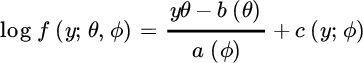
for parametrization (θ, ϕ) with θ the parameter of interest and ϕ a nuisance parameter, and some functions b only depending on θ, and a and c only depending on ϕ.
Typical examples are
- the Poisson distribution with
for which

 , a(ϕ) = ϕ = 1,
  , and
, and  !
! - the binomial model with
for which

 , a(ϕ) = ϕ = 1,
  , and
, and 
- the negative binomial model as introduced in (5.2.12) with t = 1 satisfies
so that

 , a(ϕ) = ϕ = 1,
  , and
, and  . Hence the negative binomial example only belongs to the exponential family for known α.
This family can be treated using classical likelihood theory stating that with

one has
from which we obtain that
since U = (Y − b(θ))/a(ϕ) and U′ = −b″(θ)/a(ϕ). Hence ϕ is a dispersion parameter, while b′(θ) gives the expected value of the variable Y:
- in the Poisson case we obtain the well‐known results

- in the binomial setting

- in the negative binomial case

These results confirm the underdispersion in case of the binomial model and the overdispersion in the negative binomial case as it was already found for all mixed Poisson models.
Now the expected value ![]() can be modelled as a function of a covariate (vector), either in a parametric or non‐parametric way. Here we consider the application with accident year or claim arrival year t as a covariate. While in practice the non‐parametric approach often gives a start, we first discuss here the parametric modelling approach since the non‐parametric solution uses the theory behind the parametric analysis.
can be modelled as a function of a covariate (vector), either in a parametric or non‐parametric way. Here we consider the application with accident year or claim arrival year t as a covariate. While in practice the non‐parametric approach often gives a start, we first discuss here the parametric modelling approach since the non‐parametric solution uses the theory behind the parametric analysis.
- Parametric modelling happens through generalized linear models (GLM). A standard reference here is McCullagh and Nelder [566]. A GLM allows the transformation of the systematic part of a model without changing the distribution of the variable under consideration. The link function g connects the mean μi of the observed variables Yi, i = 1, …, n, with the covariate. Assuming a simple linear predictor we then propose
where g is a smooth monotonic function and t1, …, tn are the values of the covariate. For instance, when using the Poisson or negative binomial model for Y,

 is a popular link function. The linear predictors
are used in maximizing the log‐likelihood based on the vector y = (y1, …, yn) of observations

where Θ = (θ1, …, θn), and θi = (g∘b′)−1(ηi) denotes the inverse function of the composition of g and b′. The functions a, b and c may vary with i, for instance to allow different binomial parameters n = ni for each observation of a binomial response or to allow for different α in the negative binomial model. Also, for practical work, it suffices to consider ai(ϕ) = ϕ/ωi where the weights ωi are known constants. It will often be convenient to consider Var(Y) as a function of
 , and then we can define a function V such that V (μ) = b″(θ)/ω so that Var(Y) = V (μ)ϕ.
Likelihood maximization then proceeds by partial differentiation of ℓ with respect to each β parameter:

Moreover

where the last step follows from ∂μ/∂θ = b″(θ). Hence

and the equations to solve are

These equations are in fact the solving equations of non‐linear least squares regression analysis with objective function
 , where μi depends non‐linearly on the β parameters. This set of equations is then solved iteratively. In many cases the nature of the response distribution is not known precisely, and it is only possible to specify the relationship between the variance and the mean of the responses, that is, the function V can be specified, but little more. Then, quasi‐likelihood using the log quasi‐likelihood
leads to exactly the same equations as the full likelihood approach.
As a goodness‐of‐fit criterion the scaled deviance

is proposed, which constitutes twice the difference between the maximum achievable log‐likelihood obtained by setting
 , and that achieved by the model under investigation. Moreover it can be shown that for large enough sample size n
where dim(β) denotes the number of regression parameters β. In our example dim(β0, β1) = 2.
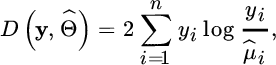
The scaled deviance based on the fitted model can be written as
with
 denoting the estimates of the parameters θi based on the full model with n parameters with maximum achievable likelihood ℓ(y;y). Here
  is known as the deviance for the current model.
Hence based on (5.5.27) and (5.5.28) we find an estimator for the parameter ϕ:
Another important goodness‐of‐fit measure for a given regression model is the explained deviance

where D(no regression) denotes the deviance for the model with only an intercept ηi = β0 (i = 1, …, n). This generalizes the adjustment coefficient in classical linear regression and expresses which percentage of the total deviance before regression has been explained by using a regression model, which is the complement of how much unexplained deviance remains after using the postulated regression model.
Finally, when ϕ is unknown, nested GLMs with p0 and p1 (p0 < p1) parameters (and corresponding deviances denoted by D0 and D1) can be compared with the generalized likelihood ratio test, rejecting [H0: model with p0 parameters holds] for large values of

with
 under H0.
- Poisson model: The deviance of the Poisson model is given by
If a constant term is included in the model it can be shown that

 , and hence then
which for large μ can be approximated by

which is the so‐called Pearson χ2 statistic.
Overdispersion can be deduced from fitting a Poisson model with which the ϕ parameter using (5.5.29) is larger than 1.
- Negative binomial model: here the log‐likelihood is given by
from which a maximum likelihood estimator of α can be traced back through a non‐linear equation involving the digamma function. The deviance is then given by


- Poisson model: The deviance of the Poisson model is given by
- Non‐parametric modelling can be performed using generalized additive modelling (GAM) where the expected counts are modelled through a smooth non‐parametric function
 not depending on specific parameters. Here the linear predictor predicts through some smooth monotonic function of the expected value of the response, and the response may follow any exponential family distribution, or simply have a mean‐variance relationship permitting to use the quasi‐likelihood approach. The resulting model is then of the kind
Given knot locations s1 < s2 < … < sm, one defines a basis b1(t) = 1, b2(t) = t, bi+2(t) (i = 1, …, m − 2) where bi+2(t) denote cubic splines linked to the knots. Then, the function h at ti is estimated through
not depending on specific parameters. Here the linear predictor predicts through some smooth monotonic function of the expected value of the response, and the response may follow any exponential family distribution, or simply have a mean‐variance relationship permitting to use the quasi‐likelihood approach. The resulting model is then of the kind
Given knot locations s1 < s2 < … < sm, one defines a basis b1(t) = 1, b2(t) = t, bi+2(t) (i = 1, …, m − 2) where bi+2(t) denote cubic splines linked to the knots. Then, the function h at ti is estimated through which yields a generalized linear model in the unknown parameters β1, …, βm. This then leads to minimizing the penalized objective function using a smoothing parameter λ which controls the weight to be given to the smoothing:
 with β = (β1, …, βm)t and S a symmetric m × m matrix only depending on the knots. Such analysis allows to validate a parametric proposal for the shape of a parametric regression function of λ or μ. We refer to Wood [795] for more details.


Figure 5.3 Dutch fire insurance data, claim counts: time plot of the yearly occurrences (top); non‐homogeneous Poisson and negative binomial fits using GAM on μi, together with horizontal line from Poisson fit with no regression μi = μ (bottom).

Figure 5.4 MTPL data for Company A, claim counts: time plot of the yearly occurrences (top); non‐homogeneous Poisson and negative binomial fits using GAM on μi, together with horizontal line from Poisson fit with no regression μi = μ (middle); Poisson and negative binomial fits with exposure as offset (bottom).

Figure 5.5 MTPL data for Company B, claim counts: time plot of the yearly occurrences (top); non‐homogeneous Poisson and negative binomial fits using GAM on μi, together with horizontal line from Poisson fit with no regression μi = μ (bottom).
5.5.2 Modelling the Claim Arrival Process
If one has more refined information on the times of claim occurrences, and hence the waiting times between these events, one can analyze the Poisson properties for these data based on the order statistics property and the independence and exponentiality of the waiting times Wi, i = 1, …, n. To verify the order statistics property one plots the time points Tj against j:
This plot should closely follow the line ![]() , where
, where ![]() denotes the average waiting time, as an estimate of 1/λ. This line hence represents how the arrival times increase with the claim number if the intensity were constant. Linearity corresponds to the uniform distribution of the arrival times over the interval [0, T] where T represents the end of the inspected time interval. Deviation from this linear structure is then a first indication that the counting process is not a homogeneous Poisson process. A formal statistical test on uniformity can, for instance, be performed using the Kolmogorov–Smirnov test for uniformity comparing the empirical distribution function
denotes the average waiting time, as an estimate of 1/λ. This line hence represents how the arrival times increase with the claim number if the intensity were constant. Linearity corresponds to the uniform distribution of the arrival times over the interval [0, T] where T represents the end of the inspected time interval. Deviation from this linear structure is then a first indication that the counting process is not a homogeneous Poisson process. A formal statistical test on uniformity can, for instance, be performed using the Kolmogorov–Smirnov test for uniformity comparing the empirical distribution function ![]() against the c.d.f. t/T of the uniform [0, T] distribution, rejecting uniformity for too large values of
against the c.d.f. t/T of the uniform [0, T] distribution, rejecting uniformity for too large values of ![]() .
.
The exponentiality of the waiting times Wi can also be verified through the exponential QQ‐plot of these inter‐arrival times:

A formal test for exponentiality based on the exponential QQ‐plot is given by the Shapiro–Wilk test based on the correlation coefficient rQ of this QQ‐plot and rejecting exponentiality for too low values of rQ. Of course graphically one can also inspect for a constant derivative of mean excess plot based on the observed W values.
In order to see how the intensity λ varies over time one can use a moving average approach, plotting

against i (i = 1, …, n). Of course under a simple Poisson counting process no trends should be visible in such plots. If deviations from a homogeneous Poisson behavior are detected in the plots, one can start evaluating the inhomogenous Poisson behavior and try to estimate the mean value function  through (5.5.32). Then after a time change using the inverse function μ−1(t) one can validate the homogeneous Poisson behavior of the time‐changed process in order to inspect possible inhomogeneous Poisson behavior.
When large clusters of arrivals appear that cannot be predicted using an inhomogeneous Poisson behavior, a next option is to consider Cox process models, for instance directed by a Lévy subordinator. In this setting Zhang and Kou [806] proposed estimating ![]() using a kernel estimator based on the observed arrival times
using a kernel estimator based on the observed arrival times ![]() in the observed time window [0, T]
in the observed time window [0, T]

with bandwidth h.
For the estimation of a Cox process directed by a Lévy subordinator model such as the gamma or inverse Gaussian subordinators, we assume that the process N is observed up to a time horizon T > 0 on a discrete time grid 0 := t0 < t1 < … < tm := T with m monitoring points. Moreover we assume an equidistant grid with step size h = T/m, that is, ti = hi for i = 0, 1, …, m. For instance the grid size could be a day or 1 week. We denote the observations of N, or the observed frequencies, at times ti as
while ![]() . Following the Lévy property of such process N the increments
. Following the Lévy property of such process N the increments ![]() (i = 1, …, m) are i.i.d. observations of the infinitely divisible distribution N(h). Using (5.2.16) we find that the log likelihood of the Cox process with the intensity parameter λ of the underlying Poisson process Ñ and the parameter vector Θ of the Lévy subordinator (i.e., Θ = (α, β) in the gamma case, and Θ = (β, η) in the inverse Gaussian model) is given by
(i = 1, …, m) are i.i.d. observations of the infinitely divisible distribution N(h). Using (5.2.16) we find that the log likelihood of the Cox process with the intensity parameter λ of the underlying Poisson process Ñ and the parameter vector Θ of the Lévy subordinator (i.e., Θ = (α, β) in the gamma case, and Θ = (β, η) in the inverse Gaussian model) is given by

This results in optimizing

with respect to (λ, Θ).
Note that the intensity parameter λ can be selected upfront assuming time normalization as the sample mean of the process distribution

Figure 5.6 Dutch fire insurance data: distribution of time points (5.5.30) (top left); moving average estimates of intensity function (with m = 50) (top right); estimated time transformation (middle left); moving average estimates of intensity function after time transformation (middle right); exponential QQ‐plot (5.5.31) based on μ‐transformed waiting times (bottom left); boxplots of monthly mean waiting times after time transformation (bottom right).
To explore the seasonality effect further, a seasonal ARIMA model is fitted to the observed intensities (e.g., see Shumway [699] or Box and Jenkins [158]). Given that many days did not have a claim at all, the data were divided into one‐week intervals. The average waiting time per week is then used as an estimate of 1/λ in that week.
A seasonal ARIMA process, or SARIMA(p, d, q)(P, D, Q)m process Xt, is an ARIMA (p, d, q) process where the residuals ɛt are ARIMA(P, D, Q) with respect to lag m:

where LmXt = Xt−m, L = L1, while ϕi, Φi are constants that determine the autocorrelation of the process with past values, and θi, Θi modulate how much past shocks have impacted on the current value. All ɛt are assumed to be i.i.d. normally distributed with mean 0 and constant variance σ2. The seasonality of the data can be inspected using an auto‐correlation function (ACF), which is defined for any process with mean μt and variance ![]() as
as

In a seasonal process one expects significant auto‐correlation with the data from the previous corresponding season. The partial auto‐correlation function (PACF) is defined as the auto‐correlation conditional on all values of the process between s and t, which eliminates the correlation originating from the values of X between s and t. Using the function auto.arima in R, an ARIMA(2, 1, 1)(0, 0, 1)52 model with mean 0 is selected given by
with ![]() . When looking for a seasonal ARIMA with lag 26 the resulting model ARIMA(2, 1, 1)(0, 0, 1)26 is
. When looking for a seasonal ARIMA with lag 26 the resulting model ARIMA(2, 1, 1)(0, 0, 1)26 is

with ![]() . In Figure 5.7 we contrast the observed intensities with a simulated process from model (5.5.34), and add the ACF and PACF plots as well as a normal QQ‐plot of the residuals of the fitted model. The observed data seem to show larger clustering. Process (5.5.34) also generates negative intensity values, which of course is not admissible. The normality of the residuals is also strongly rejected, with a correlation of 0.75 on the normal QQ‐plot of the residuals. Several power transformations were therefore used, leading to an ARIMA(2, 1, 1)(0, 0, 2)26 model based on the log‐transformed intensities:
. In Figure 5.7 we contrast the observed intensities with a simulated process from model (5.5.34), and add the ACF and PACF plots as well as a normal QQ‐plot of the residuals of the fitted model. The observed data seem to show larger clustering. Process (5.5.34) also generates negative intensity values, which of course is not admissible. The normality of the residuals is also strongly rejected, with a correlation of 0.75 on the normal QQ‐plot of the residuals. Several power transformations were therefore used, leading to an ARIMA(2, 1, 1)(0, 0, 2)26 model based on the log‐transformed intensities:

with ![]() . Now the correlation coefficient of the normal QQ‐plot of the residuals is 0.95, and the clusters are better approximated using (5.5.35), but still the clustering is underestimated.
. Now the correlation coefficient of the normal QQ‐plot of the residuals is 0.95, and the clusters are better approximated using (5.5.35), but still the clustering is underestimated.


Figure 5.7 Dutch fire insurance data. Model (5.5.34) fit: observed and simulated intensities (top left); normal QQ‐plot of residuals (top right); auto‐correlation (second line left); partial auto‐correlation (second line right). Model (5.5.35) fit: observed and simulated intensities (third line left); normal QQ‐plot of residuals (third line right); auto‐correlation (bottom left); partial auto‐correlation (bottom right).
Applying the likelihood method based on (5.5.33) using a daily observation grid over the entire observation period using a gamma and an inverse Gaussian model leads to the following parameters:
- gamma:
 ,
,  and
and 
- inverse Gaussian:
 ,
,  and
and  .
.
We simulated 100 sample paths from the fitted Cox models in order to construct confidence intervals at each time point. Both models do fit inside these bands, while the log‐likelihood values in the fitted parameters are − 3633.67 for the gamma model and − 3634.07 for the inverse Gaussian model. In order to evaluate the fit of these models, the Cox models directed by the gamma model were applied locally using a moving window of 30 days. The recorded mean values of the estimated local processes are also given in Figure 5.8, in which no stochastic structure was detected. The exponentiality of the waiting times between clusters also appears to be satisfied, and simulated processes based on the inverse Gaussian fit show similar cluster sizes, as illustrated in Figure 1.9.

Figure 5.8 Dutch fire insurance data. Simulated confidence intervals and observed cumulative counting data for fitted Cox models directed by a gamma Lévy subordinator (top left) and an inverse Gaussian Lévy subordinator (top right); mean values of locally fitted Cox gamma models using 30 days moving windows (middle left) and exponential QQ‐plot based on waiting times between clusters (middle right); cluster sizes of a simulated claim number process following the Cox model with the IG fitted parameters (bottom).

Figure 5.9 MTPL data for Company A: distribution of time points (5.5.30) (top left); moving average estimates of intensity function (with m = 50) (top right); estimated time transformation (middle left); moving average estimates of intensity function after time transformation (middle right); exponential QQ‐plot (5.5.31) based on μ‐transformed waiting times (bottom left); boxplots of monthly mean waiting times after time transformation (bottom right).
Applying the likelihood method based on (5.5.33) to using a daily observation grid over the entire observation period using a gamma and an inverse Gaussian model leads to the following parameters:
- gamma:
 ,
,  and
and 
- inverse Gaussian:
 ,
,  and
and  .
.
Again we simulated 100 sample paths from the fitted Cox models in order to construct confidence intervals at each time point. Both models do fit inside these bands, while the log‐likelihood values in the fitted parameters are almost equal: − 2462.77 for the gamma model and − 2462.73 for the inverse Gaussian model. In order to evaluate the fit of these models, the Cox models directed by the gamma model were applied locally using a moving window of 30 days. The recorded mean values of the estimated local processes are also given in Figure 5.10, in which no stochastic structure was detected. Also the exponentiality of the waiting times between clusters appears to be satisfied, and simulated processes based on the inverse Gaussian fit (see Figure 5.10) show similar cluster sizes as in Figure 1.8.

Figure 5.10 MTPL data for Company A: Simulated confidence intervals and observed cumulative counting data for fitted Cox models directed by a gamma Lévy subordinator (top left) and an inverse Gaussian Lévy subordinator (top right); mean values of locally fitted Cox gamma models using 30 days moving windows (second line) and exponential QQ‐plot based on waiting times between clusters (third line); cluster sizes of a simulated claim number process following the Cox model with the IG fitted parameters (bottom).
For the estimation of a multivariate Cox process directed by a Lévy subordinator we again assume that the multivariate process N is observed up to a time horizon T > 0 on a discrete time grid 0 := t0 < t1 < … < tm := T with m monitoring equidistant grid points with step size h = T/m, that is, ti = hi for i = 0, 1, …, m. We denote the observations of N, or the observed frequencies, at times ti as
while ![]() . Following the Lévy property of such a process N, the increments
. Following the Lévy property of such a process N, the increments ![]() (j = 1, …, m) are i.i.d. observations of the infinitely divisible distribution N(h). Using (5.2.18) optimizing the log likelihood of the Cox process with the intensity parameter vector λ of the underlying Poisson process Ñλ and the parameter vector Θ of the Lévy subordinator (i.e., Θ = (α, β) in the gamma case, and Θ = (β, η) in the inverse Gaussian model) results in optimizing
(j = 1, …, m) are i.i.d. observations of the infinitely divisible distribution N(h). Using (5.2.18) optimizing the log likelihood of the Cox process with the intensity parameter vector λ of the underlying Poisson process Ñλ and the parameter vector Θ of the Lévy subordinator (i.e., Θ = (α, β) in the gamma case, and Θ = (β, η) in the inverse Gaussian model) results in optimizing

with respect to λ, Θ.
Here, the use of time normalization means
| λ1 | λ2 | λ3 | ||
| inverse Gaussian | 180.9 | 152.6 | 56.0 |
|
| gamma | 180.9 | 152.6 | 56.0 |
|
5.6 Claim Numbers under Reinsurance
In this section we look at the number of claims when reinsurance has been taken. If {N(t);t ≥ 0} denotes the number of original claims, then after reinsurance the insurer keeps {ND(t);t ≥ 0} while the reinsurer gets {NR(t);t ≥ 0}. For all but XL reinsurance, the latter quantities are easily determined in terms of the former. We therefore deal with the XL case in a separate subsection.
- In the case of QS reinsurance the reinsurer accepts a portion a of all first‐line claims Xi, while the first‐line insurer keeps 1 − a of these claims, but then

- When there is a SL reinsurance contract with retention C, then the first‐line insurer has to deal with all the incoming claims while for the reinsurer
Indeed the reinsurer will only see one (aggregate) claim if the total claim amount in the original portfolio exceeds the threshold. However, in practice the reinsurer may also want to look into the settlement of (at least the larger) claims, leading to a big aggregate loss.

- For surplus reinsurance the situation is somewhat more complex. The first‐line insurer has to deal with all incoming claims since he can only shift part of an incoming claim to the reinsurer if the sum insured Q overshoots the retention line M. Therefore ND(t) = N(t). The reinsurer will only see the claims for which Q > M. This means that for the reinsurer the number of incoming claims equals the number of original claims for which Q > M. Correspondingly, if we have a distribution of Q available, NR(t) can be determined as in Section 5.6.1, with
 .
.
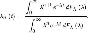
5.6.1 Number of Claims under Excess‐loss Reinsurance
Under an XL contract, the first‐line insurer has to pay the part of each claim that is below the retention, so that ND(t) = N(t). On the other hand, the reinsurer only has to pay for claims which touch the reinsured layer. Let ![]() be the probability that a claim exceeds the retention level u. Then
be the probability that a claim exceeds the retention level u. Then
with

Here ![]() denotes the probability that there are exactly k claims occurring in the time interval from 0 to t.
denotes the probability that there are exactly k claims occurring in the time interval from 0 to t.
An alternative expression can be obtained if we look at the generating function ![]() . It is a straightforward calculation to relate it to the generating function
. It is a straightforward calculation to relate it to the generating function ![]() of the original claim number:
of the original claim number:
Written in this fashion, the variable NR(t) can be considered as a thinned version of the original N(t).
From the above, one can quickly derive information on the moments of NR(t). For any non‐negative integer k

In particular
For the dispersion one has
which indicates that the smaller su, the closer the dispersion gets to the value 1, which constitutes the Poisson case (this, by the way, is a neat way to intuitively see why the Poisson distribution is a natural model for rare events).
Let us illustrate the above procedure for a number of examples that have been introduced in the previous part.
- Our first example refers to the mixed Poisson process. If we look at the reinsured part then clearly,
This simple relation shows that we only need to replace the time‐variable t by sut (i.e., a “slowing down” of the original claim number process). All other ingredients of the original mixed Poisson process remain the same. For example, generally
 Let us illustrate the above with two special cases.
- For the Pólya process we have

- For the Sichel process we obtain the generating function

- For the Pólya process we have
- For an infinitely divisible process we again look at what happens with the thinned process. From (5.6.38) we get
which can be rewritten in the form
 where
where and
and It takes a little extra calculation to see that
 where
The latter formula can in itself be interpreted as a thinning of the original variable G. We therefore see that the thinned process remains infinitely divisible.
where
The latter formula can in itself be interpreted as a thinning of the original variable G. We therefore see that the thinned process remains infinitely divisible.
- For the Neyman‐type A‐process, the thinned process is of the same type but needs
 as a new parameter.
 - Similarly for the Pólya–Aeppli process, the thinned process is of the same type with
 .
.
- For the Neyman‐type A‐process, the thinned process is of the same type but needs
- Next we deal with the Sparre Andersen model. In renewal theory thinning occurs by deleting each epoch of the renewal process with a fixed probability su, independently of the renewal process. The thinned process is a counting process that jumps at the time points
 and for n ≥ 1,
  . This thinned process is again a renewal process, now generated by the mixture

- Finally we return to the (a,b,1) class of Section 5.4. From the equations (5.6.38) and (5.4.24), some elementary algebra leads to
(5.6.39)where

 remains the same as before and where
 and
and Hence the three subcases in Section 5.4 remain invariant under the given type of thinning, one just needs to adapt the parameters. Also, the binomial and the Engen cases remain invariant. Correspondingly, the distributions of claim numbers for the insurer and for the reinsurer then only differ by the applied parameters (and for this parameter change the quantity su plays a crucuial role). This is a further reason for the popularity of these claim count models in insurance and reinsurance modelling. A convenient general class of probability generating functions that remain invariant under thinning (including many zero inflated models) is discussed in Klugman et al. [492, Sec. 8.1], where also strong mixed Poisson characterizations of the class are given.
5.7 Notes and Bibliography
Classical models for claim numbers have been studied in various textbooks on actuarial science and statistics, for example Grandell [405, 406], Klugman et al. [491], Denuit et al. [276], and Mikosch [577]. In terms of the probability generating functions, the focus here was put on moments (i.e., z = 1), whereas one may also like to consider the probabilities (z = 0), for example Sundt and Vernic [722]. Linking discrete‐time and continuous‐time models is less commonly treated in actuarial circles even if it has a long tradition in collective risk theory. Ammeter [36] proposed a model where at equidistant time instants the value of the intensity is sampled anew from some given distribution. This model (often referred to as the Ammeter model) provides a simple form of a Cox process which is another alternative to embed discrete claim counts of mixed Poisson type within a continuous‐time framework (with Cox processes directed by Lévy subordinators being a somewhat more general approach to that end). Björk and Grandell [138] considered an extension of [36] where the time instants of changing the intensity value are randomized as well, and Asmussen [56] studied a more general version in a Markovian framework, where subsequent intensities can possibly be dependent (see also Schmidli [673]). The concept of subordination is a classical topic in the theory and application of Lévy processes, for example Schoutens [683] or Kyprianou [521], but its explicit application to insurance claim processes was only taken up recently by Selch [695], even if infinitely divisible processes have been considered for many years. For an application of this joint subordination approach in mathematical finance, see Luciano and Schoutens [549].
An interesting argument for the use of mixed Poisson distributions is that if the data collected are thinned (e.g., due to a per claim deductible), then the mixed Poisson distribution is the only distribution that guarantees that also the resulting distribution of the original (non‐thinned) number of claims is a valid probability distribution (see [492, p. 122]). A discussion on different interpretations of Pólya processes can also be found in Kozubowski and Podgorski [500]. The Pólya process also has been advocated in situations where there is some kind of claim contagion (cf. Panjer et al. [600]).
The order statistics property of the Poisson process actually holds more generally for the mixed Poisson process as well as the Yule process (but not for many further processes). It is very convenient for incorporating inflation and payment delays into the analysis (cf. [492, Ch. 9]) and also appears implicitly in density representations (see also Landriault et al. [527]). It can be useful to extend properties from the marginal to the conditional setting.
Shot‐noise driven processes are classical examples of Cox processes used in the actuarial literature. For a recent reference in catastrophe modelling, see Schmidt [678] (see also Albrecher and Asmussen [14].
The (a, b, 1) class has been introduced in an attempt to gather a variety of classical claim number distributions under the same umbrella. Willmot [784] reconsidered the equation and added a number of overlooked solutions. We point out that the recursion relation (5.4.22) can easily be generalized. For specific instances, see Willmot et al. [787], Schröter [684], and Sundt [719]. For a recent contribution and further references, see Hess et al. [438] and Gerhold et al. [388].
The section on statistical approaches is developed alongside the considered models and there is clearly a lot of potential for future research work.
There are conceptual links with approaches in the credit modelling context, for example Duffie et al. [311]. Maximum likelihood estimation for compound claim count distributions is quite tractable analytically with the help of generating functions (see Douglas [307] and Willmot and Sprott [788]). Badescu et al. [71] suggest modelling the claim number process together with its reporting delay as a marked Cox process, which allows for fluctuations in the exposure.
Simultaneous modelling of dependent portfolios becomes an increasingly important topic in practice. In addition to the recent contributions on multivariate Cox process modelling mentioned in this chapter, we also refer to Sundt and Vernic [722] for an overview of higher‐dimensional approaches in terms of recursions. See also to Bäuerle and Grübel [91] and Genest and Neslehova [381] for early references to copula models. For common shock models, see, Wang [772], Lindskog and McNeil [545], and Meyers [576].