An important question when setting up a reinsurance contract with

(7.0.1)

is to determine the appropriate premium P_R(t) that the cedent has to pay to the reinsurer for entering the contract. If P(t) is the premium that the cedent received from the policyholders for risk S(t), then P_D(t) = P(t) − P_R(t) is the part of P(t) that compensates the cedent for keeping D(t), that is, we have to identify the premium sharing that goes along with the risk‐sharing mechanism (7.0.1). Since reinsurance is after all a form of insurance, one can expect similar principles to be applied for reinsurance pricing as there are for first‐line insurance. There are, however, also substantial differences to pricing for first‐line insurance, for instance with respect to

• the available data situation underlying a decision about the premium
• the degree of asymmetry of information between the two parties in the contract on the underlying risk and the corresponding data
• the way in which the long‐term relationship between the parties influences the pricing (profit participation, adaptations of risk‐sharing rules in case of severe claim experience, etc.)
• the demand and supply pattern for finding reinsurance coverage (particularly also the availability of alternatives to reinsurance, cf. Section 10.2)
• the risk of moral hazard for certain reinsurance forms.

Also, there has to be an agreement of how to share administrative costs for the acquisition of insurance policies and the settlement of claims, which is usually done by the cedent. In proportional reinsurance, this is taken into account in the form of a reinsurance commission, which will reduce the reinsurance premium (cf. Section 7.3). Due to the nature of the reinsurance market (with less available loss experience, fewer companies, limited diversification possibilities etc.), premiums will in general be adapted much faster to the loss experience than in the primary insurance market, and correspondingly market cycles (e.g., caused by the occurrence or the lack of catastrophic events) play a prominent role (e.g., see Meier and Outreville [569, 570]).

As for premiums in primary insurance markets, an actuarial reinsurance premium will typically consist of the expected loss of the underlying risk plus a safety loading.¹ In Section 7.1 we review the classical principles to determine such a safety loading, and Section 7.2.2 discusses how to include the cost of capital and solvency requirements in these considerations. We will then deal with pricing issues for proportional reinsurance in Section 7.3, and study challenges of non‐proportional treaties in Section 7.4.

The final reinsurance premium also has to contain a margin for additional costs like administrative costs, participation in acquisition expenses, runoff expenses, taxes, asset management fees, and finally profit.

We mention that there are further factors particular to reinsurance that will influence the size of the loading in the premium. In Chapter 1, a list of possible motivations to take reinsurance was given, and the relative importance of these in a particular situation will clearly have a considerable impact on the premium level that can be agreed on. In addition to that, there is a possible remaining basis risk for the cedent, that even if the reinsurance treaty is designed on an indemnity principle, there can be clauses to fix a participation amount for future corrections of the original claim size, and so the actual costs may differ from the respective reinsured amount. This risk may also be priced in. Another issue is counterparty risk: the necessary solvency capital for a cedent with respect to counterparty risk (e.g., as required in Solvency II) is influenced by the rating of the reinsurance company, and if this rating is not favorable, the cedent may ask for a premium reduction or a deposit (e.g., see Sherris [697]). Also, the concrete risk appetite of the top management on both the cedent’s and the reinsurer’s side will have an impact on the willingness to enter a treaty for a certain premium. Finally, under competitive conditions the market demand will determine which premiums can be charged, and the premium calculation procedures based on the stochastic nature of the risks will then mainly serve as lower limit prices at which offering the product becomes viable for the reinsurer. In the sequel we will not explicitly deal with these additional factors (but see Antal [43] for more details).

In this chapter we mainly focus on the (traditional) actuarial approach to pricing, dealing with the liabilities from the underwriting of risks. For the final implementation, this approach will have to be combined with financial pricing techniques, also taking into account the capital investments and its management, potential further regulatory constraints as well as economic valuation principles. Among the key drivers to determine prices will then be to maximize the resulting market value of the company, for instance using capital asset pricing models and their adaptations to insurance or option pricing techniques explicitly taking into account the possible default of the company (e.g., see Bauer et al. [89]). Some further comments on this will be given in Section 10.3.

7.1 Classical Principles of Premium Calculation

Before selling insurance and buying reinsurance, the insurer has to adopt some kind of assessment of the riskiness of the overall position. In particular, if a rule can be formulated that assigns to the claim S(t) a premium P(t) = ψ(S(t)) for some functional ψ under which the position becomes acceptable (in terms of both profitability and safety), then this defines a premium calculation principle. After reinsurance, the same analysis has to be done for the remaining position D(t). The reinsurer will have to do a similar analysis for the risk R(t), albeit with a possibly different function ψ reflecting a different risk attitude, different access to markets and hence diversification possibilities etc. In order to discuss this in general, consider the risk Y with c.d.f. F_Y, where Y could be any of the above quantities or also a single risk that is considered. If we denote the premium by P(Y), then this functional might satisfy a variety of properties that make the premium principle acceptable. Examples include:

• positive loading:
• no‐ripoff:
• no unjustified risk loading: P(Y = b) = 1 implies that P(Y) = b
• positive homogeneity: P(aY) = aP(Y) for any real constant a > 0
• translation invariance: P(Y + b) = P(Y) + b for any real constant b.

Other properties are phrased in terms of two risks Y₁ and Y₂ with c.d.f. and , respectively:

• monotonicity: P(Y₁) ≤ P(Y₂) if for all x
• subadditivity: P(Y₁ + Y₂) ≤ P(Y₁) + P(Y₂)
• additivity: P(Y₁ + Y₂) = P(Y₁) + P(Y₂) if Y₁ and Y₂ are independent
• comonotonic additivity: P(Y₁ + Y₂) = P(Y₁) + P(Y₂) if Y₁ and Y₂ are comonotonic (i.e., they can both be expressed as an increasing function of one single random variable)
• convexity: P(p Y₁ + (1 − p) Y₂) ≤ p P(Y₁) + (1 − p) P(Y₂) for any 0 < p < 1.

Not all of these properties are necessarily desirable in all situations. As an example, while positive homogeneity may look natural in terms of switching between currencies, it will often not make sense when one thinks of a as a huge number reflecting a scaled‐up risk.²

We now list some popular examples of premium principles.

• The expected value principle is given by
  (7.1.2)
  where θ > 0 is a fixed constant. So here the safety loading is proportional to the expected claim size. This principle is very popular, both due to its transparency and simplicity, and especially in reinsurance portfolios the reliability of information on the risk beyond the first moment is often limited. For θ = 0 one talks about the pure premium.³
• If information on the variance of Y is available, then another common principle is to choose the safety loading proportional to that variance:
  (7.1.3)
  which is called the variance principle, where α_V is a positive constant (for a guideline on how to choose this constant see Section 7.5).
• If the variance is replaced by the standard deviation, we get the standard deviation principle
  (7.1.4)
  where again α_S is a positive quantity. The switch from the variance to the standard deviation may be considered natural in view of underlying (currency) units: if the expectation is in €, the variance will be in €², whereas the standard deviation is also in units of € (on the other hand, one may also assume the constant α_V to be in units of 1/€, see Section 7.5 for a concrete example). Eventually, measuring variability by variance or by standard deviation gives just different weight to “additional” risk and in that sense is a matter of taste and choice. In any case, the resulting properties of the two principles differ substantially. Both are in fact used extensively, depending on the context.
• The above principles use only the first two moments of Y. If information on the entire Laplace transform of Y is available, then the exponential principle
  (7.1.5)
  (for some fixed risk aversion coefficient a > 0) has many appealing properties. One notices, however, that such a principle can only be applied to risks Y with an exponentially bounded tail, as the Laplace transform has to be finite at the positive value a.
• Classical utility theory suggests using the zero utility principle, under which the premium is determined as the solution of the equation
  (7.1.6)
  where u(x) is the utility (for the entity offering insurance) of having capital x, whereas w is the (deterministic) current surplus and P(Y) is the premium for which this entity is indifferent about entering the contract in the sense of expected utility. The utility function is usually non‐decreasing, indicating that larger risks should be counteracted by larger premiums; it is also typically concave, indicating risk aversion. If Var (Y) is small, one can approximate
  

  that is, the utility principle has some similarity to the variance principle (cf. [383]).

  For a linear utility function u, (7.1.6) gives back the pure premium, and for u(x) = −e^−ax the value of w becomes irrelevant and one finds the exponential principle again. Other frequent choices for u are power functions and logarithmic functions.

  If u is a refracted linear function with u(x) = (1 + θ)x for x < 0 and u(x) = x for x ≥ 0 for some parameter θ > 0, then for w = 0 the criterion (7.1.6) gives the expectile principle

  

  that is, the loading is proportional to the expected loss. Another way to write this is , that is, the premium is determined in such a way that when entering the contract, the “expected gain” is a multiple (1 + θ) of the “expected loss” (e.g., see Gerber et al. [386]).

  In the presence of other risks in the portfolio, it is actually more natural to assume that the current surplus is not a deterministic quantity, but itself a random variable W. In this case (7.1.6) translates into

  

  and the resulting premium will depend on the joint distribution of Y and W (i.e., on the diversification potential of adding Y to the portfolio). For instance, exponential utility u(x) = −e^−ax then gives

  

  which for small risk aversion a leads to the approximation

  

  (e.g., see Gerber and Pafumi [387]).

  While the idea of this approach is theoretically quite attractive (since under the weak assumptions stated in the classical von Neumann–Morgenstern theory a preference among two random future cash‐flows can always be expressed as a larger respective expected utility), the determination of the appropriate utility function describing the risk attitude for all magnitudes will in practice typically not be feasible. For a recent approach for insurance pricing involving utility functions beyond a concave shape see Bernard et al. [122].

• The mean value principle is defined by
  (7.1.7)
  where v an increasing and convex valuation function with inverse . For v(x) = e^rx we get again the exponential principle, while for v(x) = x we find the pure premium.
• Another approach is to distort the distribution of Y by transforming some of its probability mass to the right, in that way making the risk more dangerous. Then the premium can be obtained by taking the expected value of the modified random variable. If this distortion is done by an exponential function, one obtains the Esscher premium principle
  
  for some positive parameter h. It is clear that the Esscher principle can only be invoked for claims which have an exponentially bounded tail.
• A more general toolkit arises from distorting the distribution tail of Y. Let g be a non‐negative, non‐decreasing, and concave function such that g(0) = 0, g(1) = 1. Then the risk‐adjusted premium principle is defined by
  
  The choice g(t) = t^β is referred to as proportional hazard transform (e.g., see Wang [769]). Note that this principle can also be applied for heavy‐tailed risks.

Distorting the loss random variable provides a natural link to arbitrage‐free pricing when integrating financial aspects in the pricing mechanism (cf. Section 10.3).

Needless to say there are many other premium principles, each with some merits and defects (see the further references at the end of the chapter).

7.2 Solvency Considerations

The premium principles discussed in Section 7.1 are guidelines that can be applied to the individual risks, but also to the aggregate risk in the portfolio. However, the question of premium calculation is also intimately connected with solvency considerations, and on the aggregate level there has to be an appropriate interplay between received premiums and additionally available capital to ensure a solvent business.⁴ Then, in a next step, the aggregate premium can be sub‐divided on the individual policies. The premium principle used for this second sub‐dividing step does not necessarily have to coincide with the one applied for determining the aggregate premium (cf. Section 7.5 below).

We will now discuss two solvency criteria for determining the aggregate premium, the first one mainly for intuitive and historical reasons, the second one being the currently relevant one for many regulatory systems in practice.

7.2.1 The Ruin Probability

A traditional approach to look at the safety of an insurance portfolio is to consider its surplus process C(t) as a function of time, and observe whether this process ever becomes negative (an event that is referred to as ruin).^5,6 If at time t = 0, one starts with capital w, then the (infinite‐time) ruin probability is defined as

and the finite‐time ruin probability up to time T is correspondingly

Concretely, the ruin probability quantifies the risk of “running out of money” in the portfolio within the considered time period. In order to determine this quantity, one needs to specify the properties of the stochastic process C(t). The simpler the chosen model for C(t), the more explicit expressions one can expect for ψ(w) and ψ(w, T). If one assumes stationarity (or some sort of regenerative property) for C(t) as well as a certain degree of independence between increments of this process, then one can often apply recursive techniques, leading to integral (or integro‐differential) equations for ψ(w) and ψ(w, T), which in some cases can be solved explicitly. Such explicit formulas are then helpful to determine model parameters (in particular the invoked premium) in such a way that a target value ɛ for the ruin probability can be achieved.

The classical model for C(t) in this context is the Cramér–Lundberg model

(7.2.8)

where the premiums are assumed to arrive continuously over time according to a constant premium intensity c and the aggregate claim size up to time t follows a compound Poisson process with rate λ (see Figure 7.1 for a sample path). Infinite‐time ruin can only be avoided if the drift of the process is positive, that is,

(7.2.9)

for some (relative) safety loading θ > 0. This model is clearly very simplistic, but it enables an explicit expression for the ruin probability of the form

(7.2.10)

for each w ≥ 0, where is the n‐fold convolution of the integrated tail (or equilibrium) c.d.f.

(7.2.11)

For particular models for the claim size distribution, this expression can simplify further significantly, for example if X is exponentially distributed with parameter ν, then for each w ≥ 0

which is a simple and fully explicit formula in terms of the model parameters. In particular, for a fixed bound ψ(w) ≤ ɛ, one can – for given initial capital – determine the necessary (relative) safety loading θ in the premiums in view of (7.2.9).⁷ Alternatively, for a fixed premium c one can determine the necessary initial capital w to ensure the bound ɛ.

If the so‐called adjustment equation

(7.2.12)

has a positive solution r = γ > 0 (which requires an exponentially bounded tail of the claim size distribution^8,9), then one can show that for all w ≥ 0

(7.2.13)

This is the famous Lundberg inequality and γ is referred to as the adjustment coefficient (or Lundberg coefficient).¹⁰ If the Lundberg coefficient exists, by combining (7.2.12) and (7.1.5) one can write

for the aggregate claim up to time t, that is, the premium principle in this model can be interpreted also as an exponential principle with risk aversion coefficient γ.

If one now wants to ensure an upper bound ψ(w) ≤ e^{−γ w}  = ɛ, then one can translate the given security level ɛ and the initial capital w into the corresponding necessary adjustment coefficient , which leads to the premium requirement

Consequently, the use of the exponential premium principle and the concrete choice of its risk aversion coefficient have a motivation in the framework of infinite‐time ruin probabilities (cf. Dhaene et al. [284]).

The above considerations rely on the assumptions of the Cramér–Lundberg model, which – for the sake of simplicity and mathematical elegance – ignores many aspects that are relevant in insurance practice, including the claim settlement procedure and loss reserving (claims are not paid immediately), inflation and interest, investments in the financial market, varying portfolio size, dependence between risks, later capital injections, dividend payments etc. Many variants of the Cramér–Lundberg model which include such features have been developed in the academic literature over recent decades, leading to nice and challenging mathematical problems. However, the resulting formulas (or algorithms) typically become much more complicated, even if some driving principles can be extended to models with surprising generality (see Asmussen and Albrecher [57] for a detailed survey).

If the model incorporates so many factors that analytical or even numerical tractability is lost, one can still simulate sample paths of the resulting process C(t) and approximate ψ(w) or ψ(w, T) numerically (see also Chapter 9). However, apart from the complexity of the resulting calculations, there are other reasons that make the direct application of the ruin theory approach for solvency considerations less appealing. One of them is that it may be very difficult to formulate the dynamics of the stochastic process C(t) sufficiently explicitly so that the result can reflect the company’s situation (and the resulting model uncertainty may be considerable). This also includes the discrete nature of many model ingredients (the data situation may be sufficient to model a one‐year aggregate view, but not the dynamics within the year). Furthermore, for infinite‐time ruin considerations, there may not be a good reason to believe that business will continue in the long term in the same way as it does in the short term. Yet, the ruin probability can still provide insight into the portfolio situation: to value a certain strategy says something about how robust such a strategy is in the long run if it were continued that way (and this is a relevant question for sustainable risk management, even if one adapts the strategies later). In addition, the ruin probability quantifies the diversification possibilities of risks over time. Whereas the accounting standards in place in many countries nowadays do not allow for time diversification (e.g., equalization reserves), they can be an indispensable tool in the management of risks with heavy tails or risks where the diversification possibilities in space are limited, a situation that can be quite typical for reinsurance companies. In that sense, ruin probability calculations (or simulations) can be a valuable complement in the assessment of reinsurance solutions and their consequences.

We will come back to ruin theory considerations in Chapter 8 when the choice of reinsurance is discussed, particularly because it played a considerable role historically and is still implicitly behind the intuition of certain choices of reinsurance treaties nowadays.

7.2.2 One‐year Time Horizon and Cost of Capital

The current regulatory approach employed in most countries is simpler and considers a time horizon of one year only. Let Z(t) denote the available capital (assets minus liabilities) at time t. In broad terms, the criterion at time 0 is to hold sufficient capital so that the risky position Z(1) becomes acceptable according to some risk measure ρ. Concretely, if L(1) = Z(0) − Z(1) denotes the loss during the following year (leaving aside discounting), then the capital requirement is ρ(L(1)). For Solvency II, which has been implemented in the European Union since 1 January 2016, this risk measure determining the required capital is the Value‐at‐Risk

for α = 0.995. That is, under this requirement the probability that the loss of next year can not be covered by the available capital is bounded by 0.005. The Swiss Solvency Test, in contrast, uses the conditional tail expectation

(7.2.15)

for α = 0.99 (see also Section 4.6). In this case, even when one of the scenarios beyond the 99% quantile happens, the expected loss then still can be covered by the available capital.¹¹

There are many sources of risk that influence the distribution of L(1) in practice, so that its determination is complex. This includes also the challenge of the valuation of the assets and of the liabilities, which is supposed to be done in a market‐consistent way. Among the risk sources are market risk (volatility of equity prices, interest rates, exchange rates, etc.), counterparty risk (the risk of default or rating changes of counterparties), and insurance risk. Typically these risks are investigated separately and then combined using some assumptions on their dependence.

For the purpose of pricing, we now focus on the insurance risk in a non‐life portfolio and for simplicity assume that there is only new insurance business, which is also settled within the year (the arguments can then be adapted to include the loss development of business from previous years). Let us hence assume that the loss L(1) here is determined by the aggregate insurance loss S(1) minus the collected premium P(1) received for the respective policies. This will lead to a regulatory solvency capital requirement SCR(1) = ρ(L(1)), which the insurance company needs to hold. The capital SCR(1) will typically be provided by the shareholders of the company or external investors. For this risky investment they will demand a certain return rate r_CoC, leading to costs r_CoC ⋅SCR(1).¹²

One can now interpret P(1) as being composed of the expected claim size (referred to as best estimate) and the safety loading RM(1) (referred to as risk margin). Following the regulatory view, one can see the necessary safety loading as the amount to finance the needed capital, that is,

since then the regulatory requirement for pursuing the insurance business is fulfilled (see also Section 8.3). If the investors are the shareholders of the company and any premium in excess of claim payments at the end of the year is their profit, then r_CoC can also be interpreted as the expected return rate on their investment SCR(1).

Summarizing, with such a premium P(1) both the expected scenario and “adverse” claim situations up to the safety level of the regulatory capital requirement are covered. The need and size of the safety loading can accordingly be interpreted this way (rather than considerations of long‐term safety, as in classical ruin theory).¹³

Entering a reinsurance treaty, the insurer’s aggregate claim switches from S(1) to D(1), and correspondingly he will face a reduced expected claim size BE _D(1) and correspondingly smaller SCR _D(1), with a respective capital cost reduction. If this cost reduction exceeds the reinsurance premium which one has to invest to achieve this reduction, the resulting contract is worthwhile entering for the insurer.

Let us now look more closely at the pricing of different reinsurance forms.

7.3 Pricing Proportional Reinsurance

For proportional reinsurance treaties, the premium calculation is a priori quite simple, as it is natural to share the premium P(t) according to the same proportion as the risk S(t), and this is indeed the driving guiding principle. For a QS treaty R(t) = a ⋅ S(t) one correspondingly has

and for surplus treaties one can determine the premium share in line with the respective proportionality factor that applies for each policy (or rather class of policies). However, a number of additional items have to be considered in practice. The most important is the reinsurance commission that will be subtracted from the reinsurance premium. It compensates the cedent for the fact that acquisition costs of policies, costs for the estimation, and settlement of the claims as well as other administrative costs are carried by the cedent, and the reinsurer will participate in those to some extent. The concrete amount of participation is often made dependent on the actual loss experience:

• sliding scale commissions: after setting a provisional commission (in terms of a percentage) and a reference loss ratio¹⁴, for each percentage point that the actual loss ratio deviates from that reference point, the commission percentage is adapted (not necessarily 1:1) inversely with the loss ratio, but within upper and lower limits
• profit sharing provisions: if the reinsurer’s participation in a given year is very successful (i.e., there are few losses), the reinsurer passes back some of the premium, again along predefined terms
• loss corridors: to further protect the reinsurer, an agreement may be that the reinsurer only covers a% of the reinsurer’s loss ratio, and then again on from b% (b > a), whereas the cedent retains the part in between.

When these loss‐dependent features are defined in a piecewise linear fashion, then the calculation of their impact is still fairly straightforward, but depend on the distribution of the loss ratio. So to settle the amount of the commission, this distribution needs to be estimated from information on historical data. Here some care is needed. If the treaty is of a “losses occurring” type, then the earned premium and the accident year losses are relevant. On the other hand, a treaty can be of the “risks attaching” type, in which case losses on policies written during the treaty period are covered, and the written premium and the losses of all those policies should be considered. In a next step, catastrophe losses (which caused many claims) and shock losses (which caused single very large claims) are then most often removed from the set of collected data. Then the remaining historical losses have to be developed to ultimate values, both for the number of claims (IBNR) and the sizes of claims (IBNR and IBNER) (see also Section 7.4.2.3). In addition, the historical premiums have to be adjusted to the future level, including the rate changes that are expected during the treaty period. Finally, the losses also have to be trended to the future period. From all these obtained data points, the expected loss ratio is then estimated by the arithmetic average of the respective historical loss ratios adjusted to the future level. At this point, a catastrophe loading then has to be added to the expected non‐catastrophe loss ratio, for which various methods are used, including simulation models (e.g., see Clark [215, 216] for details).

Finally, in certain lines of business the reinsurer may actually have a lot, sometimes more, experience in the nature of the claims, and may want to adapt or correct the premium amount collected by the cedent to the size that he deems more appropriate.

7.4 Pricing Non‐proportional Reinsurance

From an actuarial point of view, the pricing of non‐proportional reinsurance is considerably more involved than that for proportional treaties. As mentioned before, the more reliable information one has about the claim size distribution, the more flexibility one gains in terms of using a premium principle like the ones mentioned in Section 7.1. In typical non‐proportional reinsurance treaties, one often has difficulties in determining more than the first one or two moments, so that an expected value principle or variance principle is quite common. In addition, a number of clauses (including reinstatement constructions etc.) often even make the determination of the first two moments a non‐straightforward assignment. We will therefore discuss some guiding principles for determining the pure reinsurance premium. Two main approaches can be distinguished. The first is mainly based on the reinsurer’s own experience and assessment of the underlying risks, normalized to the volume of the exposure (reflected by the premium that the cedent collected from policyholders for this portfolio (exposure method)). The second relies on the previous loss experience of that particular reinsured portfolio (experience method).

We focus here on XL treaties (for SL the same principles apply). For more information on large claim reinsurance forms, refer to Section 10.1.

7.4.1 Exposure Rating

7.4.1.1 The Exposure Curve

Consider an individual claim X, which is subdivided into X = D + R. Recall from (2.3.9) that under an xs M contract we have

(7.4.16)

This shows that if one is interested in the pure reinsurance premium in such a treaty, the function

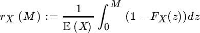
is particularly useful, as it gives for each retention M > 0 the fraction of the risk X that stays with the cedent. r_X(M) is called the exposure curve. Mathematically, one immediately recognizes r_X(M) as the equilibrium distribution function of X, which leads to nice properties. For instance, for the Laplace transform one has

where is the Laplace transform of X. In particular, there is a one‐to‐one correspondence between F_X and r_X. From r_X^′(x) > 0, r_X^″(x) < 0 one sees that the exposure curve is an increasing and concave function (and, as the c.d.f. of a positive random variable, it starts in 0 and tends to 1 for ).

Even if in light of this one‐to‐one correspondence one does not gain directly from modelling the exposure curve (instead of the distribution of X), it will turn out to be a quite useful description below, and actuaries have developed a remarkable intuition about the shape of this curve for certain lines of business. Note that for the aggregate claim size in a portfolio with i.i.d. risks X_i, one can use the same exposure curve as for X:

as the influence of N(t) cancels out. For the direct modelling of exposure curves, one often uses discrete shapes. A continuous one‐parameter family of such curves that still enjoys some popularity was given by Bernegger [129]:

with b(c) = e^{3.1−0.15(1+c)c} and g(c) = e^{(0.78+0.12c)c} for a parameter c (which is often chosen to be one of the values c ∈{1.5, 2, 3, 4}, but other values are used as well). Note that here x is in % of the size of the risk, measured, for example, by the sum insured or the PML (see Section 7.4.1.2).

The exposure curve plays a crucial role in determining the pure reinsurance premium.

7.4.1.2 Pure Premiums

The idea in exposure rating for the reinsurer is to consider the insurer’s pure premium P_j for each different risk group j and then use own experience (that the reinsurer may have gained through previous treaties in that market), experience from related portfolios or market statistics to determine the premium. That “experience” is reflected in the choice of the exposure curve. For an contract on risk group j one then gets

and for an L xs M contract correspondingly

That is, one has intuitive and simple adaptations of the insurer’s premiums available. Such an approach is only feasible if the chosen exposure curve r_j applies to all risks of that risk group, an assumption that may only be fulfilled if the sizes Q_i of the risks in the policies underlying the claims X_i are sufficiently similar. If this is not the case, there are two common adaptations:

1. If the loss degree V_i = X_i/Q_i can be assumed to be i.i.d. across the policies (which seems a reasonable assumption in property, marine hull and personal accident insurance¹⁵), then one can estimate (or use from past sources) the exposure curve r_V for the loss degree directly to get for an treaty
   
   A particular advantage in this case is the fact that r_V is inflation‐invariant and currency‐invariant (as inflation will affect M and Q_i in the same way).
2. In liability insurance the sum insured will often be chosen arbitrarily and is typically much smaller than the maximum claim size, so that the above assumption is not reasonable. One may then, however, assume that the original risk X is identically distributed within the same risk class, and that the claim for each policy is just truncated at different values Q_i, that is, for some generic non‐truncated X with exposure curve r_X. One then obtains
   
   which is referred to as the increased limits factors curve (ILF curve). But here r_X is not inflation‐ and currency‐invariant, which is undesirable. An alternative reasoning going back to Riebesell [648] proposes that when doubling any insured sum, the pure premium should be multiplied by 1 + z for some fixed 0 < z < 1, that is, (in contrast to property insurance above where the insured sum is a measure of the size of the risk, here the pure premium increases less than the sum insured). This rule then implies
   

   which is again inflation‐ and currency‐invariant (see Mack and Fackler [556] for a characterization of distributions of X for which this logarithmic scaling rule of can indeed be fully justified). The resulting reinsurance premium then again is

   

   For further extensions and discussions see Riegel [649] and Fackler [343].

As for proportional treaties, in addition the reinsurer may want to correct the used values of P_i if he does not consider them appropriate.

7.4.1.3 Safety Loadings

To determine the safety loading, it is often the variance that is of interest (if available). For this purpose, for an L xs M contract a natural possibility is to use the representation

introduced in (6.5.24), where N_R(t) is the number of claims that the reinsurer faces, an is the reinsured amount of the jth claim that concerns the reinsurer. Let (note that this differs from introduced in Section 2.3.1, as does not have an atom at 0). If one assumes i.i.d. claim sizes, then

where is the pure premium from the previous section. Hence, the variance can be expressed in terms of the exposure curve in the region of the layer. Note that (particularly for higher layers) will often be close to 1, so the second term in the above sum can be quite small.

In Section 7.5 we will deal with the determination of safety loadings from an aggregate point of view.

7.4.2 Experience Rating

In contrast to the exposure method, in experience rating one bases the calculations on the loss experience of the concrete portfolio. This can work if there is sufficient credible claim experience available. In this context the techniques introduced in Chapter 4 can be very useful. As already discussed there, the insurer will typically not pass on the entire series of previous claims, but only those that are immediately relevant for the layer under consideration (so that the reinsurer faces the statistical challenge of data analysis under truncation). For instance, only past claims larger than half of the deductible over the last 5–10 years would be communicated. In order to make those past data points comparable, they have to be suitably adjusted. Each considered factor may influence the size of the claims, the number of the claims or both. Besides changes in legislation, technical changes or changing insurance market conditions (which are sometimes not easy to incorporate), the following three factors need to be considered and can typically be quantified to a satisfactory degree.

7.4.2.1 Inflation

Data points spreading over several years need to be inflation‐corrected. Depending on the line of business, there may also be other adjustment indices that are more suitable (like the building cost index). This makes the data points comparable, but there is also another important aspect of inflation in XL treaties: a claim that previously did not touch the layer under consideration may nowadays be above M, that is, relevant for the treaty (this is the main reason for the reporting threshold for past claim sizes to be considerably below M and not at M). To see this, consider the expectation in an L xs M contract. After inflation with factor δ > 1 this changes to

that is, the latter corresponds to the (scaled) expected reinsured claim size in the layer [M/δ, (M + L)/δ]. In typical cases this resulting expectation is larger than the inflation‐corrected original expected value. For instance, if X is strict Pareto with parameters α > 1 and x₀, a simple calculation gives .

The inflation may affect the claim sizes and the claim number in different ways, which complicates the analysis. Inflation can be a major issue in MTPL lines (for a detailed discussion see Fackler [342]).

7.4.2.2 Portfolio Size Changes

In a next step, all data points have to be adjusted to the portfolio volume of the present year. After correcting for tariff adjustments, the premium amount is often considered a suitable measure for the volume, particularly in fire and motor liability portfolios (although inflation may affect premiums and claim sizes differently, which also has to be taken into account). For fire, the sum insured (or PML) is also used (see also Section 7.4.1). In other lines of business, other measures may be considered more natural (like passenger kilometers flown in aviation liability). Whether the claim sizes are assumed to increase proportionally with volume or with respect to some other functional relationship, and whether this affects both the sizes and the number of claims, strongly depends on the line of business and the type of cover (e.g., for per‐risk XL, volume will typically affect the number of claims and not the size, whereas for cumulative XL it will rather influence the size of the (aggregate) claims per event).

7.4.2.3 Loss Development

In some lines of business (and particularly so in liability), it can take many years until a claim payment is finally settled. In such a case, one has – for all claims that are not fully developed yet – only development patterns and current estimates of the final loss burden available. The reinsurer then needs to use loss reserving techniques on an individual claim basis in order to make the data points of different years comparable. This needs to be done both for the number of claims (IBNR) and the sizes of the claims (IBNR and IBNER) (see Chapters 1 and 4, where this is discussed in detail and illustrated with data). One may finally also have to discount the data according to the typical payment patterns, as later payments enable to invest the premiums until the payments are due.

If all these adaptations are done and one is left with comparable data points, then the simplest procedure is to build the empirical c.d.f. and use it for the pricing (this is called burning cost rating). The resulting expected claim size (i.e., the arithmetic mean of the data points, correspondingly referred to as burning cost) is often considered quite useful, but clearly the empirical distribution will typically not be sufficient to model the entire risk (using the empirical c.d.f. implies that the largest possible claim size has already occurred!). Also, one often has rather few data points in the layer. We refer to Chapter 4 where we have discussed and illustrated respective EVT techniques extensively. Also, a Bayesian approach with an a priori guess for model parameters (such as the extremal index) is sometimes implemented. Finally, credibility techniques can be quite useful, where a weighted average is taken between the own claim experience and the one of related portfolios. The weights are chosen according to how “credible” the respective claim information is, and the development of respective algorithms is a classical actuarial technique (see the references at the end of the chapter).

If there is no relevant claim experience available at all, but one has an estimate of how frequently a loss occurs (say once in n years), then a crude way to state a pure premium is to divide the layer size L by n. This leads to a payback tariff (the contract is said to have an n‐years payback, see also Section 2.3.3).

7.4.3 Aggregate Pure Premium

If one finally has distributions for the individual reinsured claim sizes R_i and the claim number N(t) available, then the aggregate claim size distribution for the reinsurer can be determined just as for the first‐line insurer. In the presence of an aggregate (typically annual) deductible AAD and an aggregate limit AAL we have

(cf. (2.3.14)). For instance, if all risks are i.i.d. and N(t) is Poisson or negative binomial, then the distribution of can be determined by Panjer recursion (cf. Section 6.3). The aggregate pure premium for the XL treaty is then obtained through

(7.4.17)

As discussed before, in XL practice often the premium is not fixed in advance, but dependent on the loss experience during the contract. In that case, the (pure) premium rule is then the function P which satisfies

(7.4.18)

Examples are contracts with the following:

• Slides: For a slide with a fixed loading L_s, the agreement is of the form
  
  that is, the reinsurance premium actually is the aggregate claim experience R(t) of the reinsurer plus the loading L_s, but capped at a minimal and maximal premium values P_min and P_max, respectively. One way to implement this is that for given P_min, loading L_s and distribution of R(t), the value of P_max is determined such that (7.4.18) holds.

  Alternatively, a slide with proportional loading b is a contract of the form

  
• Reinstatements: This variant of XL contracts has already been discussed in Section 2.3.2. The sequence (c_n)_1≤n≤k is fixed in advance and called a premium plan, that is, further liabilities may have a different price than the first one. The values c_n may be fixed (pro‐rata capita) or depend on the time when the reinstatements are paid (pro‐rata temporis). The latter variant is intuitive, since close to the expiry of a contract it will be less likely that the next liability will be used up, but this is nowadays not so common anymore. For the reinstatement of the nth such liability (n ≤ k) one then has
  
  For pricing under different premium schemes, see Mata [562] and Hess and Schmidt [439].

7.5 The Aggregate Risk Margin

The risk margin that the reinsurer needs to put on top of the pure premium and the expenses will of course also depend on the other risks in the reinsurer’s portfolio (in view of diversification possibilities etc.). We will take here the viewpoint of Section 7.2.2 and assume that the reinsurer has a required cost‐of‐capital rate r_COC (i.e., a return target on risk‐adjusted capital), which in view of his overall situation leads to the aggregate risk margin RM := RM(1). This amount now has to be sub‐divided onto the risk margins of all m treaties that the reinsurer has in the portfolio:

where RM_j denotes the risk margin of treaty j with risk R_j (so ). Theoretically, the classical rule

appears natural. However, knowledge about the covariance between treaty j and the aggregate risk R(1) will most often be out of reach, so one has to resort to simpler rules.¹⁶ A typical compromise for such a simpler rule is to consider the fluctuations of each treaty stand‐alone, for example in terms of the variance principle

(which is exactly the above covariance principle for independent reinsurance treaties) or in terms of the standard deviation principle

A further possibility is the square root rate on‐line (ROL) principle: if L_j denotes the aggregate upper limit of the reinsurer in treaty j, then for the ROL (cf. Section 2.3.3), one divides according to

Recall that the philosophy behind the ROL is that it approximates the probability of a total loss L_j of the layer. If one assumes that either no claim or the total loss L_j occurs for treaty j, then one would get , and (for small r_j) the principle then resembles the standard deviation principle above.¹⁷

A challenge in the implementation of the above approach in practice is that at the time of the pricing of treaty j, one often does not yet know which other treaties will be added to the portfolio, so that one has to estimate the constant α_V, α_S or α_R, respectively, for the future portfolio on the basis of the current composition and planned modifications. The resulting constant can then be used to price each of the treaties according to the respective premium principle (so this provides a concrete guideline for the choice of the constants α_V and α_S in Section 7.1).

One issue that remains is the following inconsistency: if the layer L_j of treaty j were subdivided into two layers, then (due to the positive dependence of the loss in these two layers) the variance of the loss of the entire layer would be larger than the sum of the variances of the two sublayers (and similarly for standard deviation and ROL). That is, there is (at least theoretically) an incentive for the cedent to chop the layers into smaller and smaller pieces whenever such a premium principle is applied. One suggestion to mitigate this non‐additivity is the so‐called infinitesimal ROL principle: starting again from the aggregate pure premium (7.4.17)

where is the aggregate reinsured claim size in treaty j in the absence of aggregate deductible and limit, the idea is to apply the ROL principle separately for each small part (z, z + Δz) ∈ [M_j, M_j + L_j], that is,

and in the limit Δz → 0 one gets . The infinitesimal contribution to the premium according to the ROL principle then is , so that the overall contribution amounts to

and the constant α_R^* is analogously RM divided by the sum of all these m integrals. By construction this method to allocate the risk margins does not suffer from the non‐additivity problem.

The idea of deriving the individual risk margins (loadings) from its marginal capital requirements can be traced back to Kreps [507]. The capital allocation for the individual layers is often done using the so‐called capacity appetite limit (CAL) curve, which assigns the risk weights to different tranches of capital. This CAL curve can be seen as the reinsurer’s implicit utility function and is provided to the pricing team by overall capital considerations. For more refined pricing techniques in view of capital considerations see [689].

7.6 Leading and Following Reinsurers

In many realizations of reinsurance contracts there are in fact several reinsurers involved in a treaty. A leading reinsurer negotiates the premium, but finally only takes a certain proportional share of both the premium and the risk, and other reinsurers take the remaining proportions. If we again assume that there are m treaties and the reinsurer’s share in treaty j is a_j ≤ 1, then the aggregate risk for the reinsurer is

As a consequence, the risk margin then is determined by the premium calculation of the leading reinsurer.¹⁸

If an overall premium P_j for a reinsurance treaty R_j is already negotiated, a (following) reinsurer has to determine on the basis of his internal premium principle, if and to what extent a participation in that treaty is feasible. For fixed costs k involved in entering the contract, one gets the condition

for the internal premium rule P, on the basis of which one can determine which share a_j is appropriate (or optimal). When the reinsurer internally employs a standard deviation principle, this leads to a linear inequality for a_j (such that the optimal share is the maximum available share), whereas for a variance principle the resulting inequality is quadratic in a_j.

In terms of leading and following reinsurers it is quite common that all reinsurers equally participate in all layers (“across the board”). If one of the reinsurers does not want to take the equal share in the upper layers (e.g., due to internal limits) or lower layers (because of high administrative costs due to the large number of claims there), then this can be passed on to one of the other reinsurance partners or a reinsurance broker looks for an external additional reinsurer to take part in only those layers.

7.7 Notes and Bibliography

For general classical accounts on premium calculation in risk theory we refer to Gerber [383], Goovaerts et al. [400], and Kaas et al. [476]. For a more applied view see Mack [555] and Parodi [606]. An early discussion of convexity in the context of premium calculation is Deprez and Gerber [279]. An ordering using Lorenz curves was discussed in Denuit et al. [278], see also Heilmann [434]. An extension of the expected value principle to a quasi‐mean value principle with its properties is given in Hürlimann [454].

Reich [642] has shown that the standard deviation principle enjoys some fundamental properties. Benktander [111] suggests a linear combination of expected value, variance, standard deviation principles.

The distortion principle can be found in Denneberg [273] and turns out to be quite general, in the sense that many pricing rules (and risk measures) can be expressed that way for an appropriate distortion function (see Wang [770, 771], and Pflug and Römisch [615] for a general overview in the context of risk measures). Duality concepts play a major rule in this context (see Yaari [799] for a classical influential contribution). Furman and Zitikis [362] discuss the general and intuitive concept of actuarial weighted pricing functionals, which contain many pricing rules (also when related risks are considered) and propose implications for capital allocation.

Principles for calculating premiums are of course choices to measure risk, and the research area of risk measures, their axiomatic foundations, and entailed capital allocations has seen an enormous activity over the last two decades, boosted by the paper of Artzner et al. [49] on coherent risk measures. We do not give an overview of the correspondingly vast academic literature, which is often primarily targeted towards financial applications. An early axiomatic approach for insurance pricing can be found in Wang et al. [773], Venter [755], and Young [801]. An interpretation of the ruin probability concept in the context of risk measures can be found in Dhaene et al. [284], Cheridito et al. [203], and Trufin et al. [746]. As mentioned earlier, for (re)insurance purposes the VaR plays a central role in regulation, and also the CTE is a much discussed measure (and implemented in the Swiss insurance regulation). A survey of what can happen to VaR calculations when the claim size distribution has heavy‐tailed or time‐dependent behavior is given in Bams et al. [77]. Danielsson [246] covers the role of the VaR in connection with extreme returns, see also Neftci [588] and Luciano et al. [548]. The performance of extreme value theory in VaR calculations is compared to other techniques by Gençay et al. [379]. For risk measures with a pricing undertone, see Van der Hoek et al. [751]. For more details on ES as a risk measure, see Acerbi et al. [8] and Fischer [352]. Necessary and sufficient conditions for coherence are covered by Wirch and Hardy [793]. A rather general risk measure for the super‐exponential case has been developed in Goovaerts et al. [401] and is based on a generalization of the classical Markov inequality from probability theory. Siu and Yang [702] introduced a set of subjective risk measures based on a Bayesian approach. For other alternatives, see, for example, Balbás et al. [75]. Powers [625] suggests the use of the third and fourth moments to measure risk.

Despite the toolkit of techniques discussed throughout this book, the data situation on the losses of certain reinsurance portfolios often does not provide sufficient reliable distributional information beyond a few moments (if at all), and this is one of the main reasons why simple rules based on one or two moments are still abundantly used in pricing. We point out, however, that one has to be very careful when estimating empirical moments from the data points directly. As amply illustrated in Chapter 4, it may easily happen in reinsurance applications that the underlying moments that one wants to estimate do in fact not exist. For instance, when one tries to estimate the sample dispersion or (particularly) the sample coefficient of variation directly from a set of i.i.d. data points with a distribution for which the first or second moment do in fact not exist, the erratic behavior of their estimates may somewhat cancel out in the estimator of the ratio, and so one may not “see” the problem immediately and proceed with the estimate, even if the true value is not finite. This problem is illustrated in some detail in Albrecher et al. [25, 27], where asymptotic properties of the corresponding estimators in such situations are also worked out.

Brazauskas [162] deals with the effects of data uncertainty on the estimation of the expected reinsured amount under various reinsurance treaties from the viewpoint of robust statistics.

Historically, Beard [92] claimed that the most troublesome premium calculation likely to arise in practice would be the determination of an XL reinsurance premium based only on the largest claims experience. A first attempt on the use of extreme value techniques for pricing of XL treaties was made by Jung [473]. For an early practical approach including IBNR techniques, see Lippe et al. [546]. For a treatment of large claims within credibility, see Bhlmann and Jewell [171] and Kremer [504]. For information and references on credibility techniques, refer to Dannenburg et al. [247], Kaas [475], and Bühlmann and Gisler [169]. Alternative estimation procedures can be found in Schnieper [682]. The effect of contract terms on the pricing of a reinsurance contract is discussed in Stanard et al. [708].

A standard reference on stochastic ordering is Shaked et al. [696], see also Kaas et al. [475] and in particular Denuit et al. [274]. For a general account on the concept of comonotonicity, refer to Dhaene et al. [281, 282].

A rich source for practical issues in pricing of proportional reinsurance is Clark [216]. Antal [43] discusses pricing from the reinsurance perspective in detail. For refinements of exposure rating techniques for fire portfolios, see Riegel [650]. Mata [563] gives more information on burning cost methods. Verlaak et al. [761] develop a regression technique to form a benchmark market price out of individual MTPL XL prices. Desmedt and Walhin [280] suggest a method of combining exposure rating and experience rating for pricing rarely used layers through using exposure techniques on the experience rates of working layers.

The final aggregate combined ratio (defined as the ratio of the sum of incurred losses and operating expenses divided by earned premium) of reinsurance companies naturally varies widely across reinsurance companies and years, but a realistic average magnitude reported in practice is 80–90% (e.g., see [354]). Loading factors θ (cf. (7.1.2)) of individual reinsurance treaties in practice again can vary considerably, the range from θ = 0.1 in lower layers to θ = 0.6 in more extreme layers (and also outer contracts when combining reinsurance forms) is, however, typical in competitive reinsurance markets (e.g., see Verlaak and Beirlant [760]).

Pricing is also conceptually quite different between property and casualty lines: whereas the former is dominated by prefunding losses, the idea of postfunding losses underlies the pricing of casualty losses, see [375] for details on this and many other practical matters.

In life reinsurance, the standard model for pricing Cat XL layers goes back to Strickler [712], for a recent refinement see Ekheden and Höossja [319].

Note that the stop‐loss premium (defined as the expected claim size of a reinsurer in an unlimited SL cover, cf. (6.5.28)) corresponds to from (7.4.16), but applied to the c.d.f. of the aggregate claim size. Even if such unlimited covers are not often applied in reinsurance practice, the stop‐loss premium has been studied intensively in terms of its theoretical properties, and these results can be used as benchmarks. For instance, bounds on stop‐loss premiums have been studied by Bühlmann et al. [168], and Runnenburg et al. [659] under heavy‐ and light‐tailed assumptions (see also Kremer [503]). For bounds where the claim distribution is unknown but in the proximity of the empirical distribution of past claims, see Xu et al. [798]. For numerical and algorithmic aspects, see Kaas [474], and recursive methods are discussed in Dhaene et al. [287]. Also, it is of particular interest to look into robustness of stop‐loss premiums with respect to dependence of the individual claims. First studies in this direction include Dhaene and Goovaerts [283], Albers [12], and Denuit et al. [275]. The interplay between maximal stop‐loss premiums and comonotonicity is dealt with by Dhaene et al. [286]. Various approximations are compared in Reijnen et al. [643].

Pure premiums for drop‐down XL covers as introduced in Chapter 2 can be found in Kremer [506]. For a general analysis of various risk measures for reinsurance layers, see Ladoucette and Teugels [522].