
2
Reinsurance Forms and their Properties
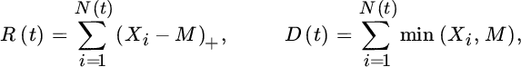
Let ![]() be random variables denoting the claim sizes that the first‐line insurer experiences and let {N(t);t ≥ 0} be a counting process, where N(t) represents the number of claims up to time t > 0 (measured in years). Then the total or aggregate claim amount at time t for the first‐line insurer is given by
be random variables denoting the claim sizes that the first‐line insurer experiences and let {N(t);t ≥ 0} be a counting process, where N(t) represents the number of claims up to time t > 0 (measured in years). Then the total or aggregate claim amount at time t for the first‐line insurer is given by

Recall that most (non‐life) contracts are written for the duration of one year, so the static random variable S(1) will be of prime interest in many applications.
In a reinsurance contract, this aggregate claim size is now sub‐divided into
where D(t) is the deductible (retained) amount that stays with the first‐line insurer after reinsurance and R(t) is the amount paid by the reinsurer. For many reinsurance contracts the splitting will be defined on the individual risks Xi, and in this case we write Xi = Di + Ri (or just X = D + R for short, in case they all follow the same distribution).
We will now discuss the most common obligatory reinsurance forms and their properties. We start with proportional (also called pro‐rata) treaties.
2.1 Quota‐share Reinsurance
The simplest possible reinsurance form is quota‐share (QS) reinsurance, which is a fully proportional sharing of the risk, that is,
for a proportionality factor 0 < a < 1.
This form of reinsurance is popular in almost all insurance branches, particularly due to its conceptual and administrative simplicity. In general the first‐line insurer will also cede to the reinsurer a similarly determined proportion of the premiums (see Chapter 7 for details). If the distribution of X is available, one immediately has

expressed in terms of the cumulative distribution function (c.d.f.) ![]() . For the aggregate risk, correspondingly
. For the aggregate risk, correspondingly
and for the moment‐generating function
so one only needs to evaluate the moment‐generating function of S(t) at a different argument. As a result, the rth moments ![]() are given by
are given by
Note that both the coefficient of variation and the skewness coefficient ν do not change under a QS treaty:


2.1.1 Some Practical Considerations
QS reinsurance can be understood as (virtually) increasing the available solvency capital. To see that in a simple example, consider the probability
that at some time t > 0 the capital v together with the received premiums P(t) suffices to cover the claims S(t). Then, after entering a QS treaty and assuming that premiums are shared with the same proportion, this probability changes to

In practice, a further positive effect of QS reinsurance is to improve the premium‐to‐surplus ratio: according to statutory accounting principles implied by the regulator, an insurer typically has to immediately include in the balance sheet all the expenses connected to issuing a policy, but the respective premium can only be entered gradually over the duration of the policy; the correspondingly needed unearned premium reserve considerably reduces the surplus and a QS arrangement will improve this situation, as it reduces that reserve and the expenses simultaneously (see, for example, [585]). QS contracts are often used at the initiation of smaller companies to broaden their chances for underwriting policies and to gain experience in a new market with a limited amount of risk. For reinsurers, in turn, a QS arrangement can also have the advantage of gaining claim experience in that particular market, which may be useful in other related portfolios.
QS arrangements are easy to combine, that is, an insurer can have simultaneous QS contracts on the same portfolio with different reinsurers. Also, due to the proportional share that is left with the insurer, the risk of some forms of moral hazard (like sloppy claim settlement procedures) is avoided.
One of the main shortcomings of QS reinsurance is that, due to its form, all claims are partly reinsured, not just the largest of them. This is often not ideal, as claims from small policies could have easily been borne by the insurer alone (and passing on those parts of the portfolio is a non‐attractive loss of insurance business).
2.2 Surplus Reinsurance
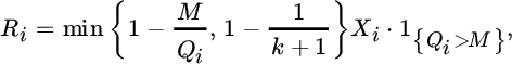
A reinsurance form that improves on the disadvantages of QS treaties, but keeps its main advantages, is surplus reinsurance, which is a proportional reinsurance form for which the proportionality factor depends on the coverage limit in the underlying policy (sum insured). Let Qi be the sum insured (policy limit) of claim Xi. For a fixed retention line M the reinsured amount is then given by

where 1{A} denotes the indicator function of event A. Altogether,

The ratio Vi := Xi/Qi is called the loss degree of claim Xi. With a surplus reinsurance each claim with an insured sum below M is fully kept by the insurer, and otherwise the relative participation of the reinsurer in the claim payment is larger the larger the underlying sum insured is (see Figure 2.1). Consequently, this reinsurance form retains the advantages of the proportionality for each claim payment, but only reinsures claims from larger policies. Due to the proportionality feature, the determination of premiums is again rather simple. In some cases Qi is alternatively the probable maximum loss (PML) of claim Xi (see Chapter 7). From the definition, it becomes clear that the maximum retained size of each claim is M (“the line”). The surplus reinsurance contract homogenizes the portfolio of the first‐line insurer, as illustrated in the following simple example.
Figure 2.1 Proportionality factor of the reinsurer as a function of insured sum.
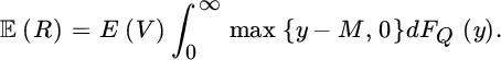
In order to determine the distributional properties of the retained and reinsured amount under surplus reinsurance, it is helpful to consider the insured amount of a claim as a random variable with (c.d.f) FQ (based on frequencies of the sums insured specified in the policies of the portfolio and the respective claim occurrence probabilities, for example in Example 2.1 Q would have a two‐point distribution with ![]() ).1 The distributions of the quantities R and D are then given by
).1 The distributions of the quantities R and D are then given by


For the moments of D, we have

In practice it may often be reasonable to assume that the loss degree is independent of the sum insured (particularly if the sums insured do not vary too much across policies). In that case, (2.2.5) simplifies to

For the reinsured amount, the respective expression is slightly more involved, but for the first moment one easily gets

and under independence of V and Q
Surplus reinsurance is very popular, particularly in fire insurance, as well as property, accident, engineering and marine insurance. Typically, there is an upper limit Qi ≤ (k + 1)M (“k lines”) in the treaty, that is, the ceded share is capped by
and the remaining part for the policies with larger sums insured is then negotiated on a facultative basis. Also, for certain policies the insurer may decide to retain several, say m < k, lines and only reinsure the remaining k − m lines (e.g., see [585]). In general, it is not uncommon to apply a table of lines, that is, different retention lines to various groups of similar risks. The retention line is then often chosen in a way to aim for the same maximum loss (method of inverse claim probability) or average loss (method of inverse rate) for each policy (cf. [526]).
2.3 Excess‐of‐loss Reinsurance
We now move on to non‐proportional reinsurance forms. The simplest case is the (per risk) excess‐of‐loss (XL) reinsurance defined by
for some pre‐defined retention M,2 that is, the reinsurer agrees to pay for each claim the excess over the retention M. Typically, this will only be agreed upon up to a certain limit L, leading to

and one refers to such a treaty as L xs M, characterized by the layer [M, M + L] (layer size L). Note that ![]() . The ratio (M + L)/M is referred to as the relative layer length.
. The ratio (M + L)/M is referred to as the relative layer length.
This reinsurance form is very popular in casualty and fire insurance, as it reduces the exposure of the ceding company in an effective way and has an intuitive and simple form. The premium calculation is, however, considerably more involved than for proportional reinsurance forms (see Chapter 7). Figure 2.2 schematically depicts the reinsured claim amounts under a QS, surplus and XL treaty.

Figure 2.2 Comparison of reinsured claim amounts for some combinations of claim sizes Xi and corresponding insured sums Qi for QS reinsurance with a = 0.3 (left), surplus reinsurance (middle), and L xs M reinsurance (right).
2.3.1 Moment Calculations
Consider the random variable
for any u, v ≥ 0. If u = M, ![]() refers to the reinsured amount R of a single risk in a v xs M treaty. On the other hand, for u = 0 and v = M,
refers to the reinsured amount R of a single risk in a v xs M treaty. On the other hand, for u = 0 and v = M, ![]() refers to
refers to ![]() in an
in an ![]() xs M contract. That is, studying distributional properties of
xs M contract. That is, studying distributional properties of ![]() will be relevant for both parties involved in the XL contract.
will be relevant for both parties involved in the XL contract.
If FX denotes the distribution function of X, then one gets

and for the Laplace transform of ![]()

For the kth moment we get

From this expression one can read off the first moments

for the retained and reinsured single claim amount in an ![]() xs M treaty, which has the appealing optical interpretation of sub‐dividing the area between FX(z) and the constant line 1 (see Figure 2.3).
xs M treaty, which has the appealing optical interpretation of sub‐dividing the area between FX(z) and the constant line 1 (see Figure 2.3).

Figure 2.3 Graphical interpretation for the splitting of the expected claim size between insurer and reinsurer.
For the case L xs M one analogously obtains

These simple expressions will play a crucial role in the pricing of XL treaties in Chapter 7. From (2.3.8) one also gets the inequalities
On the other hand,  so that
For the variance, one has

Since the partial derivative with respect to v is  , the variance is non‐decreasing in v and we get the bound

The quantity on the right is non‐increasing in u and therefore smaller than the same expression where we put u = 0, but the latter then refers to the variance of the original risk X, so that we get for any u, v ≥ 0
The coefficient of variation can be written as

and hence depends monotonically on the ratio under the square root. By (2.3.11) the derivative of that ratio is

If we write ![]() for any u, v, then it follows that
for any u, v, then it follows that
The dependence on u is more intricate. Let us introduce the retention distribution

with moments  . If we abbreviate r := FX(u + v) − FX(u) then it is easy to show that
The latter relation is handy in rewriting the partial derivative of CoV(u, v) with respect to u. Indeed, it easily follows that

but then

Replacing in the last expression the moments ![]() by their analogues νk from (2.3.13), we get
by their analogues νk from (2.3.13), we get

which is positive. Indeed, the quantity ![]() is the variance of the distribution Gu, v while by definition ν1 ≤ v. This then shows that the requested partial derivative is non‐negative and hence that CoV(u, v) is also increasing in u. In particular,
is the variance of the distribution Gu, v while by definition ν1 ≤ v. This then shows that the requested partial derivative is non‐negative and hence that CoV(u, v) is also increasing in u. In particular,
comparing the risk of the different layers. Applying the left inequality for ![]() and the right one for u = 0 we also get
and the right one for u = 0 we also get
where the quantity in the middle is the coefficient of variation for the original claim size. For moment calculations for the aggregate claims of each party under an XL treaty see Chapter 6.
2.3.2 Reinstatements
Many L xs M contracts in practice have in addition an (annual) aggregate deductible (AAD) and an (annual) aggregate limit (global layer) (AAL) (often a multiple of L), so that

In the following we assume AAD = 0 for simplicity. A very common variant (particularly in property and casualty insurance) is such a contract with k reinstatements, that is, at the beginning only an initial premium P0 for the coverage of a first “layer” (or “liability”) min{R(t), L} is paid. When a claim occurs, that layer is (partially) used up, and it can be refilled with later premium payments (reinstatement premiums) (see Example 2.2). Altogether then AAL = (k + 1)L. More details on the respective premium schemes are discussed in Section 7.4.3.

Figure 2.4 100 xs 100 treaty with one reinstatement and claims X1 = 150, X2 = 175, X3 = 225, and X4 = 150.
Note that with such a reinstatement clause, the premium payment is no longer deterministic, but depends on the loss history during the contract. Such reinstatements can be negotiated to be automatic or optional for the first‐line insurer. Clearly, this variant of XL contracts is attractive for the cedent, as some premiums only have to be paid if more coverage is needed, and there is less financial burden for the cedent in the beginning. With such clauses, it is easier to agree on premiums, and one can interpret the setup as a loss participation scheme of the cedent, which also reduces moral hazard. The actuarial analysis of such contracts is, however, more involved. Early discussions of XL contracts with reinstatements can be found in Sundt [717, 718] and Rytgaard [663]. The resulting distribution of aggregate claim sizes is studied in Walhin and Paris [767] and Hürlimann [455], and for corresponding ruin probabilities see Walhin and Paris [768] and Albrecher and Haas [417]. For the pricing of such contracts see Section 7.4.3.
2.3.3 Further Practical Considerations
There are many issues to be taken care of in the concrete implementation of an XL treaty. One is that the way in which inflation influences the retention may not be the same as for the claim sizes, and corrections of inflation effects (and implementing respective clauses in the contracts) are an integral part of XL treaty analysis (see also Chapter 7). Walhin et al. [766] provide an overview of financial, economic, and commercial aspects in the practical pricing of XL treaties. On the data side, particularly for the lines of business relevant for XL treaties (such as liability), some claims take several or even many years until settlement, so respective reserving techniques on an individual claims level have to be set up and one faces statistical challenges (see Chapter 4).
It is not uncommon to combine XL treaties with adjacent layers. In practice, one often refers to the rate on line (ROL)
and the payback period 1/ROL, which reflects the average number of years it takes to collect premiums for this layer so that one payment of the full layer is reimbursed (one distinguishes working layers (small ROL), middle layers (medium ROL), and CAT layers (high ROL); this terminology is mainly used for casualty risk). Finally, layers far in the tail are sometimes referred to as capacity layers. For property losses the respective expressions are frequency layer, estimated normal loss layer, PML layer, PML protection layer, and CAT layer.
Whereas the usual XL treaty (2.3.6) is defined per risk, this may not be an effective reinsurance form if one faces many (but possibly not excessively large) claims (frequency risk). One way to deal with this problem is a cumulative XL (per‐event XL, cat XL) contract, where first all claims that can be attributed to the same event are aggregated to  and then the reinsurer pays the excess of that aggregate claim over a specified priority Mc, that is,

Mathematically, this reduces again to an XL‐type contract, with the number of claims now replaced by the number of events and the individual claims replaced by the aggregate claim per event. That is, if there are enough data available to model the event process and the respective aggregate claim distribution for an event, one can again use the same techniques as for the per risk XL. Cumulative XL treaties are popular in property, marine hull, motor hull, personal accident, and natural catastrophe insurance.
It is evident that in XL reinsurance there is an adverse selection, namely that an insurer seeks protection particularly for risks that are hard to model or have heavy tails, but often with very limited past claim experience. Some aspects of this phenomenon will be dealt with later in the book. Another issue in practice can be moral hazard in its various forms. In addition to what was mentioned above, another example is that if a claim is already larger than the retention, there may not be the same incentives for the cedent to be very careful with the exact settlement of the claim (as this is costly). A finite layer size L is already a partial remedy to this problem, another one is that the reinsurer only pays a (pre‐specified) fraction of the original reinsured amount in the XL treaty (such contracts are sometimes referred to as change‐loss contracts).
Variants of per‐risk XL are adverse development covers (dealing with run‐offs) and industry‐loss warranties (cf. Section 10.2).
2.4 Stop‐loss Reinsurance
A stop‐loss (SL) reinsurance treaty is defined by

that is, the aggregate loss that the cedent faces over the time interval is capped at the priority C, and the reinsurer takes care of the excess. Although SL is a natural alternative to XL reinsurance that relieves the cedent from tail risk completely, some of the problems of XL (like the moral hazard issue) are even amplified for this reinsurance form. In almost all cases implemented in practice there is also an upper limit U specified in the contract:

To avoid some of the problems, such a reinsurance form is typically combined with a proportional and/or XL cover inuring to the SL treaty (i.e., the SL feature only applies to the risk remaining after the other treaties) (cf. Section 2.6). It is also common to include an additional unconditional deductible in (2.4.15) to lower the administration costs connected to very small losses.
A SL contract is particularly useful if the assignment of claims to a particular event for a per‐event XL is difficult (such as hail, agriculture or frostiness of waterpipes). However, on the administrative side such a contract can be quite tedious, as all claims have to be considered (and potentially agreed upon) by both parties and modelling for the aggregate tail can be a challenge. In addition, all small claims contribute to the reinsured amount, a feature that makes this reinsurance form less effective. As a consequence, such contracts are typically expensive and not so frequently applied (an exception being, for example, German windstorm reinsurance). A SL cover is, however, a popular reinsurance form between connected institutions. The distributional properties of a SL contract can in principle be deducted from the corresponding ones of single risks in an XL cover (cf. Section 2.3.1), but due to the clauses in the aggregation structure the analysis can in concrete cases still look quite different.
2.5 Large Claim Reinsurance
Consider the ordering of the claims
In a large claim reinsurance contract the reinsurer agrees to cover the largest r claims, where r ≥ 1 is a fixed number, that is,

This is an intuitive treaty against the risk of large claims for the cedent, and it leads to challenging mathematical questions for the distribution of R(t) and D(t), which we will discuss in some detail in Section 10.1, particularly also with respect to asymptotic properties. A variant is drop‐down XL with

where different retentions and layer sizes are applied to the respective order statistics (e.g., see Ladoucette and Teugels [522, 524]). While the implementation of such treaties seems quite reasonable, they are nevertheless not very popular in modern reinsurance practice, probably due to the intricate mathematical details and the considerable model risk, as particularly for the largest claims in the portfolio one only has limited means to justify on a statistical basis assumptions on the claim distribution. A variant of (2.5.16) that has some popularity is called second event retention (or DD), which is an XL cover, where the retention and the size of the layer also vary for different claims over time, but are then ordered by chronological appearance rather than size.
A further variant of large claim reinsurance that was implemented for some time in certain countries is called ECOMOR (Excédent du Coût Moyen Relatif). Introduced by Thépaut [742], it was defined by

that is, it is an XL‐type treaty, where the retention is given by the (r + 1)th largest claim. The respective mathematical analysis is slightly more complicated than for large claim reinsurance contracts, and we will give some details in Section 10.1.3. One motivation for the introduction of such an (a priori) random retention was the advantage that it is (by definition) prone to the same inflation forces as the claims themselves. At the same time, there is an intuitive drawback of the ECOMOR construction: if during the contract period an additional claim appears that raises the applied retention, it can happen that the reinsured amount decreases, although the overall burden for the cedent has increased by the arrival of this additional claim, a feature that is not desirable and hence moral hazard can be a problem. Up to now ECOMOR treaties have enjoyed some academic popularity due to their mathematical challenges, but these are also to some extent the reason why this reinsurance form is not used in current practice. There are, however, some reinsurance treaties in force that to some extent mimick ECOMOR features, such as an SL cover on all claims that are larger than some threshold.
2.6 Combinations of Reinsurance Forms and Global Protections
Even for a relatively simple property portfolio a combination of different types of reinsurance protections is quite common. Clearly, this complicates the analysis of the contracts and makes it even more important to clearly understand the implications of each type of contract on the shape of the retained and reinsured risk. One of the main reasons for implementing such combinations is heterogeneity. Heterogeneity is induced by the difference of sums insured per policy, but also differences in coverage (theft, third party protection, etc.) and in type (simple, commercial or industrial risks, etc.).
Combinations of proportional and non‐proportional reinsurance protections are quite frequent. If one combines non‐proportional reinsurance types, a logical order needs to be respected: first a per‐risk XL, second a per‐event XL, and finally a SL. A QS can be ceded in any order. When applied, a surplus treaty (possibly preceded by a QS) should be the first in the series. A surplus after a per‐event XL is logically impossible, while a surplus after a per‐risk XL will imply that the risks with higher sum insured, which are systematically ceded to the surplus, also have a higher potential to lead to XL payments. So one should recover parts of the XL premium on a pro rata basis from the surplus reinsurers, which entails some challenges in practice.
There seems to be an increasing trend that ceding companies ask for global protections of their portfolios. One example is the protection by the reinsurer of two (or more) lines of business, for instance of fire and MTPL. This allows better advantage to be taken of the diversification possibilities. In a multiline XL coverage, layers from different lines of business are combined in one treaty with a global (or multiline) annual aggregate deductible AAD which is taken to be rather large (to keep the reinsurer’s payments and the respective reinsurance premium in a reasonable range).
As an example consider a classical fire treaty with three layers (2000 xs 1000; 3000 xs 3000; 1000 xs 6000) with reinstatements, and a MTPL treaty with three layers (3000 xs 2000; 5000 xs 5000; ![]() xs 10000) and unlimited free reinstatements. An alternative coverage could consist of a global multiline treaty combining a fire layer 2500 xs 500 with a 4000 xs 1000 MTPL layer with unlimited free reinstatements, and a multiline retention of 1000. These two layers then form one treaty with one global premium, which is complemented by the two remaining fire layers and the two remaining MTPL layers. In order to price such a multiline coverage one needs to model the possible dependence between the different components or lines of business. Analysis of the Danish fire insurance data will be used to illustrate the multivariate joint modelling of different components.
xs 10000) and unlimited free reinstatements. An alternative coverage could consist of a global multiline treaty combining a fire layer 2500 xs 500 with a 4000 xs 1000 MTPL layer with unlimited free reinstatements, and a multiline retention of 1000. These two layers then form one treaty with one global premium, which is complemented by the two remaining fire layers and the two remaining MTPL layers. In order to price such a multiline coverage one needs to model the possible dependence between the different components or lines of business. Analysis of the Danish fire insurance data will be used to illustrate the multivariate joint modelling of different components.
2.7 Facultative Contracts
Currently about 15% of reinsurance contracts (in terms of premium volume) are not of an obligatory treaty form, but are contracts negotiated on individual risks. This includes in particular coverage for non‐standard risks such as reinsurance for skyscrapers, powerplants etc. As there are virtually no a priori rules for such contracts and the agreed risk‐sharing mechanisms can vary widely, they cannot be treated systematically. Due to their individual nature the premiums are typically considerably higher than for standardized obligatory treaties. Often, the insurer tries to avoid including risks in a treaty that are particularly prone to large losses as this may have a bad effect on premiums in the following year, and so the insurer will aim for a facultative reinsurance for those risks.
Further examples of non‐standard reinsurance forms are discussed in Section 8.8.
2.8 Notes and Bibliography
In addition to the general references already given at the end of Chapter 1, it should be noted that some reinsurance companies regularly publish online information on practical details and reinsurance market trends, see, for example, the webpages http://www.swissre.com/sigma/ and http://www.munichre.com.