
3
Models for Claim Sizes
In this chapter we deal with models that are useful for describing individual and collective claim size data and physical measurement data of natural hazards such as earthquakes and floods. Because we want to give special attention to the modelling of large claims we provide some general background on this topic. In what follows we will try to distinguish between claims that are considered small and claims that are large. It is intuitively clear that reinsurance contracts will depend heavily on whether or not the individual claims should be considered large.
3.1 Tails of Distributions
One of the main reasons for taking reinsurance is the possible appearance of large claims. While this sounds like an obvious statement, a useful and acceptable definition of what is meant by a large claim is far from obvious. Among the possible examples of distributions, some are better suited to model large claims than others. In view of future applications to actuarial topics one definitely needs a way of making a difference between average claims and large claims. An acceptable guideline is to compare claim distributions with the exponential distribution. In some sense the exponential distribution acts as a splitting distribution between small and large. A first and rather vague criterion would be to check whether the claim distribution under consideration has a fatter tail than the exponential distribution or not. If it does not, then we could call the distribution super‐exponential; in the alternative case we might call the distribution sub‐exponential but unfortunately this term has already been standardized in the probabilistic literature.
We will call a distribution F super‐exponential if 1 − F(x) is bounded above by a decreasing exponential. A more quantifiable definition can be given in terms of ![]() , the Laplace transform of F, in that
, the Laplace transform of F, in that ![]() has a strictly negative abscissa of convergence σF. Following Taylor [731] we will indeed conclude that the super‐exponential class of distributions is a reliable family of light‐tailed claim size distributions. The exponential distribution itself also satisfies this criterion of super‐exponentiality. The aggregate claim distribution (but also other risk quantities such as ruin probabilities) often exhibit exact or approximate exponential behavior when the underlying claim size distribution is super‐exponential.
has a strictly negative abscissa of convergence σF. Following Taylor [731] we will indeed conclude that the super‐exponential class of distributions is a reliable family of light‐tailed claim size distributions. The exponential distribution itself also satisfies this criterion of super‐exponentiality. The aggregate claim distribution (but also other risk quantities such as ruin probabilities) often exhibit exact or approximate exponential behavior when the underlying claim size distribution is super‐exponential.
For a distribution F with a fatter tail than any exponential the abscissa of convergence σF of ![]() will be zero. Unfortunately this property is not sufficiently specific to be useful as a definition. Instead one uses some classes of distributions with σF = 0 that have a bit more structure. In particular we will deal later with sub‐exponential distributions, Pareto‐type distributions, extreme value distributions, etc. If we take the claim size distribution from such a class, the corresponding aggregate risk and ruin quantities will show no trace of exponential behavior.
will be zero. Unfortunately this property is not sufficiently specific to be useful as a definition. Instead one uses some classes of distributions with σF = 0 that have a bit more structure. In particular we will deal later with sub‐exponential distributions, Pareto‐type distributions, extreme value distributions, etc. If we take the claim size distribution from such a class, the corresponding aggregate risk and ruin quantities will show no trace of exponential behavior.
3.2 Large Claims
Before we offer candidates for claim size distributions, we need to remind the reader that one of our main objectives is to provide adequate models for large claims. This section contains a few thoughts on what we might righteously call a large claim and how one can perhaps distinguish it from others. For an early general discussion on the role of large claims see the summary report by Albrecht [32]. For an attempt to define the even more difficult concept of a catastrophic claim, see Ajne et al. [10].
Consider all claims {X1, X2, …, Xn} related to a specific portfolio. Let ![]() be the total claim amount and consider the maximum value Xn, n. Under which conditions should we consider this largest claim to be actually large? More generally, which of the extreme order statistics could be considered to be large? For an attempt to define large, see Teugels [738]. Beirlant et al. [105] put large claims into a statistical and actuarial context. Here are some interpretations, the first two theoretically inspired.
be the total claim amount and consider the maximum value Xn, n. Under which conditions should we consider this largest claim to be actually large? More generally, which of the extreme order statistics could be considered to be large? For an attempt to define large, see Teugels [738]. Beirlant et al. [105] put large claims into a statistical and actuarial context. Here are some interpretations, the first two theoretically inspired.
- A claim could be called large when the total claim amount is predominantly determined by it. A possible interpretation would be to assume that Sn is large because Xn, n is so. This might be interpreted by the conditionFor n = 2 this is equivalent to

The last equivalence follows from

The relation (3.2.1) is precisely the definition that F belongs to the class S of sub‐exponential distributions. A property of S, proved by Chistyakov [211], is that if F∈S then for any non‐negative integer n, as
 ,(3.2.2)
In the sub‐exponential case, the tail 1 − F*n is (up to the quantity n) just as heavy as that of 1 − F.
Members of S are automatically members of the class of long‐tailed distributions1 denoted by L, which means that for all


The class S and its subclasses have been constantly used as candidates for claim size distributions with a heavy tail but also in other probabilistic contexts like branching processes, queueing theory, etc. The major drawback of S is that it is only defined in terms of a limiting property, which is hard to verify in practice, and that it is defined by a non‐parametric condition. Up to now the sub‐exponential class has defied a representation. Actually, it remains a challenging problem to decide whether a set of actuarial data comes from a sub‐exponential distribution or not. Further, it is known that S is not closed under convolution or under convex combinations. Cline and Samorodnitsky [195] have shown that nevertheless large subclasses of S are closed under product operations (see also the work by Rosinski et al. [657]). A variety of sufficient conditions for membership of S can be found in the literature, for example see Pitman [622], Teugels [737], Klüppelberg [493], Pinelis [619], Smith [704], and Foss et al. [356] for a recent survey. Refinements are available in Chover et al. [212] and Willekens [779].
Henceforth, practitioners avoid the class as such, going for distributions that are sub‐exponential but that at the same time contain enough parameters. Only then will they be able to use data. Among the many parametrized examples in S we mention the log‐normal distribution, the Pareto distribution and Pareto‐type distributions to be defined next, as well as non‐normal stable distributions.
- Another way of defining large claims can start from the behavior of the maximum claim, which is then also closely related to the concept of the PML (cf. Chapter 2). This mathematical problem was considered in the work by Fisher and Tippett [353] and Gnedenko [391], and was further streamlined by de Haan [257]. The main question is the search for distributions of X for which there exist sequences an > 0 and bn (n = 1, 2, …) such that for all real values x (at which the limit is continuous) for some non‐degenerate distribution G. It was then shown that the extreme value distributions
are the only possible limits in (3.2.3), with
 called the extreme value index (EVI). It has to be understood that Gγ has to be a proper distribution. This means in particular that the range of Gγ extends over the interval
  if γ > 0 (the Fréchet–Pareto case), over
  if γ < 0 (the extremal Weibull case), or over
  if γ = 0 (the Gumbel case).
For any specific γ, the max‐domain of attraction, containing the distributions F for which there exist sequences an > 0 and bn such that (3.2.3) holds, have also been described. The class of distributions in the max‐domain of attraction can be defined in terms of the tail quantile function. Given that F is a distribution, its quantile function is defined by the inverse function

The tail quantile functionis defined and denoted by

The following condition is a necessary and sufficient condition for the existence of normalizing and centering constants for the weak convergence (3.2.3) of the maximum of a sample from the distribution F.
Here the restriction to u ≥ 1 can be broadened to u > 0. It follows from the general theory of regularly varying functions that a is automatically regularly varying at infinity with index γ: a(x) = xγℓ(x) where ℓ is slowly varying, that is, a measurable and ultimately positive function that satisfies
for all t > 0. For more information see Bingham et al. [135].
It has been shown by de Haan in [257] that the above definition can be equivalently stated in terms of the original distribution. The alternative condition is
for all u such that 1 + γu > 0 and where h ∘ U = a. For γ = 0 we read
 . The above relation holds locally uniformly in u. Furthermore if γ > 0, then
  as
as  . However, if γ < 0, then F has a finite upper limit
  and
and  . The limit distribution in (3.2.6), that is,
is called the generalized Pareto distribution (GPD).
In case γ > 0, the class Cγ equals the class of Pareto‐type distributionsdefined by
where α = 1/γ > 0 and ℓ is slowly varying. Note that 1 − F in (3.2.7) is regularly varying with index − α.
When γ ≤ 0, the underlying X has a tail that is lighter than Pareto‐type distributions. In case γ = 0 the tail of the distribution of X can have a finite endpoint or infinite support.
Seemingly the first attempt to model large claims with a parameterized distribution is due to Benckert et al. [109]. Here the authors assume that the claim size distribution starts out as a Pareto distribution, this means that for large x, 1 − F(x) ∼ c x−α for some positive α. The distribution is then “cut off” at the point corresponding to the sum insured, in which the remaining mass of the Pareto distribution is concentrated. This then yields a model with negative γ. A bit later, Benktander [110] pointed out how the Pareto distribution itself (or its variants) could be used to model large claims. In particular he considered the Pareto class as a dividing class between claim size distributions for which all moments are finite and those for which most moments diverge. Pareto‐type distributions have always been popular, for instance when modelling fire, storm and liability data, as will be illustrated in Chapter 4. For a survey of extreme value theory and relevant references, see Embrechts et al. [329], Beirlant et al. [100], and de Haan and Ferreira [258].
- For statistical purposes one can make a distinction between tails that tend to 0 faster or slower than the exponential distribution near infinity. When for any λ > 0the tail of X is termed lighter than exponential (LTE), while for
 the tail of X is termed heavier than exponential (HTE).
- When an actuary looks at claim data, he might suspect that large claims are likely. For example, when he tries to estimate the mean and/or the variance of the claim size distribution in a sequential way, he notices that the sample estimates do not converge. Even when he uses re‐sampling techniques, the estimates fail to average out to a limiting value. One possible reason might be that the mean or the variance of the underlying claim size distribution actually does not exist because the tail of the distribution is too heavy. This could mean that the law of large numbers does not apply, preventing ultimate stabilization. A possible parameterized form to cope with such a phenomenon is to assume that F is a Pareto‐type distribution with a small index α, as considered above.
- One could call a distribution heavy tailed if the ratio Sn/Xn, n converges in distribution to a non‐degenerate limit law. This approach leads to the class of Pareto‐type distributions with 0 < α < 1, as shown by Breiman [163]. If the distribution F has a finite expected value μ then the analogous condition that (Sn − nμ)/Xn, n converges to a non‐degenerate limit leads to a similar outcome but with 1 < α < 2.
- Another possibility is that a number of the largest claims consume a fair portion of the total claim volume. In a formula, for some p ∈ (0, 1), Xn, n > pSn. Of course, the value of p should be large enough since otherwise all order statistics could be termed large. In a more general phrasing, one could look atfor a value of α close to 1. For a quantification of this approach in terms of Lorenz curves, see Aebi et al. [9].
- In a similar fashion we might interpret largeness by the condition that for some finite constant c when
 ,where ν is the mean μ if it is finite while otherwise ν is 0. As shown in Bingham et al. [136] this condition again leads to the Pareto‐type distributions with α ∈ (0, 1) ∪ (1, 2).


Before continuing we need to stress the difference between a large claim and an outlier. While the first is a genuine member of the sample of claim sizes, an outlier is considered an extraneous value. Next to clear misprints, events can occur which are completely unexpected in view of all data before such an event. Using methods from extreme value analysis (EVA) one can estimate how unlikely certain events are in view of all prior information. When events with an extremely low likelihood do occur, however, one has to be ready to change the statistical models.
3.3 Common Claim Size Distributions
In this section we state the traditional examples of claim size distributions that are commonly considered in the actuarial literature. Some of these examples are simple while others are more elaborated variations. For other surveys of common claim size distributions, see Kupper [517], Ammeter [40] and Klugman et al. [491].
In many cases, distributions can be derived from a simple original by a transformation. Among the most popular are the following:
- replacement of the random variable X by a Box–Cox transformation, that is, Yλ := (Xλ − 1)/λ, which for the limit λ = 0 gives

- replacement of X by exp(X), where the resulting distribution is called a log‐distribution
- replacement of X by a normalized version aX + b for constants a > 0 and

- replacement of X by
 with a > 0, a so‐called homeographic transformation.
Note that such transformations may dramatically change the tail behavior of the distribution.
Because of the importance of extreme values in reinsurance, the extreme value distribution Gγ, ![]() , and the generalized Pareto distribution are important candidates for modelling purposes in view of the limit results (3.2.3) and (3.2.6). The sets of extreme value distributions and generalized Pareto distributions are one‐parameter families of distributions ranging from light tails with a finite endpoint (with γ ≤ 0), up to Pareto‐type tails (when γ > 0). Applying a normalization to these families we obtain the location‐scale versions with
, and the generalized Pareto distribution are important candidates for modelling purposes in view of the limit results (3.2.3) and (3.2.6). The sets of extreme value distributions and generalized Pareto distributions are one‐parameter families of distributions ranging from light tails with a finite endpoint (with γ ≤ 0), up to Pareto‐type tails (when γ > 0). Applying a normalization to these families we obtain the location‐scale versions with ![]() and σ > 0:
and σ > 0:

and

where ![]() . The latter distribution has been used to model aggregate claim distributions in McNeil [567]. Condition (3.2.6) leads to the popular peaks‐over‐threshold (POT) approach in EVA, as discussed in Chapter 4.
. The latter distribution has been used to model aggregate claim distributions in McNeil [567]. Condition (3.2.6) leads to the popular peaks‐over‐threshold (POT) approach in EVA, as discussed in Chapter 4.
We now list a number of examples of models with tails that are exponentially bounded and then turn to tails heavier than exponential.
3.3.1 Light‐tailed Models
3.3.1.1 With EVIγ < 0
A classical example of a light‐tailed distribution with finite endpount x+ is given by the beta distribution with x+ = 1 and distribution function

with extreme value index γ = −1/q (here B(p, q) = Γ(p)Γ(q)/Γ(p + q) denotes the beta function). The uniform distribution on (0, 1) is of course a special case with p = q = 1. This is then a possible model for loss degree data. Beta distributions can be constructed starting from a Pareto‐type random variable Y (cf. (3.2.7)) through the transformation X = x+ − 1/Y leading to an extreme value index γ = −1/α:

Another way to produce a light tail with finite endpoint from a heavy‐tailed distribution W is by conditioning on W < T for some value T:
Such an operation is called here upper‐truncation.2 A first reference in this respect is Benckert et al. [109]. See Clark [217] for a reference in enterprise risk management.
With T fixed, one can show that X is then light tailed with EVI γ = −1. When modelling large claims it appears appropriate to consider T sufficiently large, possibly with the meaning of a sum insured. Another example is found in the Gutenberg–Richter model for earthquake magnitudes, as will be discussed when treating earthquake data in Chapter 4.
3.3.1.2 With EVIγ = 0: the Gumbel Domain
- Our first set of examples starts from the exponential distribution given byThe exponential distribution plays a central role in tail modelling, not least because of its memoryless property, that is, for all s, t > 0
 Since the tail quantile function of the exponential distribution equals
 , the exponential distribution belongs to C0(a), where a(t) = 1/λ. From the exponential distribution we get the following:
 - A first Box–Cox transformation of the exponential distribution is known as the Weibull distribution and is defined byFor τ > 1 the distribution is still super‐exponential. Note the special case of the Rayleigh distributionwhich is obtained by putting τ = 2. The Weibull distribution has

 as the tail quantile function so that this distribution belongs to C0(a), where
  .
. - An exponential change followed by a normalization yields the logistic distribution with explicit formwhere μ is a real parameter and σ > 0. Note that this distribution is taken on the entire real line. One‐sided versions are of course possible. The most common choice of the latter is the one‐sided logistic distribution


- A first Box–Cox transformation of the exponential distribution is known as the Weibull distribution and is defined by
- The gamma distribution also has a long tradition in claim size modelling. Its explicit form is where α, λ > 0. Further

 so that σF = −λ and hence, the gamma distribution is super‐exponential. For integer values of α the gamma distribution can be characterized as a sum of independent exponential random variables (and is then referred to as the Erlang distribution). For α = n/2 and n an integer we find a chi‐squared distribution.
 Many other special Box–Cox forms are available. We mention here the transformed gamma distribution, obtained from the gamma distribution via a power transformation. We find

a distribution with three parameters.
When there is good reason to believe that a claim comes from one of several different risk classes and for each of these classes one has a good idea about the claim size distribution, then a mixing distribution will be a natural model. In this context, mixtures of Erlang distributions are very popular in claims modelling, for example see Willmot and Woo [790]. Such mixed Erlang distributions are used in Chapter 4 to produce global fits in combination with separate tail fits. A popular, tractable and more general class of super‐exponential type in such a probabilistic construction context are phase‐type distributions (see Bladt and Nielsen [139], [57, Ch. IX] and Asmussen et al. [65] for the statistical perspective). For a recent variant of infinite‐dimensional phase‐type distributions with finitely many parameters leading to a heavy‐tailed distribution, see Bladt et al. [140].
- When modelling claim size distributions, the normal distribution can hardly be advocated as a valuable model because claim sizes are non‐negative. Nevertheless the distribution is still popular as an approximation. Some distributions derived from it have also found their way into the actuarial literature:
- The one‐sided normal distribution is a candidate, suggested already in Benktander et al. [115]. It has the density function

- The inverse Gaussian distribution is defined by the density functionwhere the two parameters β and μ are positive. Its Laplace transform is given by
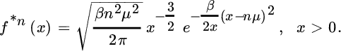
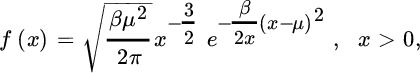 from which it is easy to see that the density of the n‐fold convolution is
- The one‐sided normal distribution is a candidate, suggested already in Benktander et al. [115]. It has the density function
Hence σF = −β/2 and the distribution is super‐exponential. For further properties see Embrechts [323]. The closedness under convolution makes this distribution an interesting candidate for claim size modelling, probably Seal [692] was the first to consider it for this purpose. Later applications can be found in Gendron et al. [380], ter Berg [736] and Mack [555].
3.3.2 Heavy‐tailed Models
3.3.2.1 With EVIγ = 0: the Gumbel Domain
- Our first examples can be derived from the exponential distribution.
- The Weibull distributionis sub‐exponential for 0 < τ < 1.

- The second Benktander distribution is defined by the expressionwhere a and c are positive constants and 0 < b < 1.

- The Weibull distribution
- Also the normal distribution can give rise to heavy tails after transformation.
- The most popular such distribution is the log‐normal distribution, defined as a two‐parameter distribution of the formHere

 while σ > 0. This important distribution belongs to S, as shown in Embrechts et al. [326], and asymptotically has a tail heavier than the Weibull distribution, namelyIn 1962, Benckert [108] suggested the use of the log‐normal distribution for the modelling of industrial and non‐industrial fire data. Ferrara [347] fitted a log‐normal distribution to fire claim data. Further specific examples have been treated in the papers by Bennett et al. [116] and Dickmann [289], and Taylor [729] also illustrated the use of the log‐normal. For an early application to windstorm and glass claims data see Ramlau‐Hansen [640].
- The quasi‐log‐normal distribution is defined by the following class containing three parameterswhere α, b and β are positive parameters. It captures the dominant component

 (for some β > 0) in the tail behavior of a log‐normal distribution.
- The most popular such distribution is the log‐normal distribution, defined as a two‐parameter distribution of the form
3.3.2.2 With EVIγ > 0
This class corresponds to the Pareto‐type distributions as defined in (3.2.7).
- By far the most popular distribution to generate heavy claims is the Pareto distribution with its transformed versions. It is the prime example of heavy‐tailed distributions. The simplest possible definition is the strict Pareto distribution given for α > 0 byThe strict Pareto is sub‐exponential for all values of α. It can also be seen as a log‐distribution generated by an exponential random variable. The fact that this distribution is only defined from a positive value x0 on, is often not considered a problem since it is mainly used to model large claims. More than that, this distribution is very popular in practice because of a certain type of lack‐of‐memory property: for any threshold M > x0 one has
 (3.3.9)that is, the conditional excess is again Pareto‐distributed, now with parameters (α, M), a property that is particularly attractive in XL reinsurance.
- The shifted Pareto distribution is a two‐parameter family defined byIt can be obtained from the strict Pareto by a simple shifting and rescaling or from the Pareto‐type by a specialization of the slowly varying function. Note that its support is now the entire positive axis. For a treatment in an actuarial context see Seal [694]. It is also known as the US–Pareto distribution in actuarial circles. The GPD is actually the special case β = 1/α.

- Adding an additional power to the shifted Pareto distribution yields the versatile Burr distribution defined byThis three‐parameter distribution has received a lot of attention in the actuarial literature. The tail quantile function of the Burr distribution is
 The distribution therefore belongs to
 , where
  . For a generalized Burr‐gamma distribution, see Beirlant et al. [103]. For α = 1 one finds the log‐logistic distribution.
 - The Fréchet distribution defined byis directly derived from the extreme value distributions (3.2.4), replacing X by 1 + γX when γ > 0, and is a popular model for heavy‐tailed data on its own.

- The gamma distribution also leads to heavy‐tailed distributions after a transformation. We mention in particular the log‐gamma distribution, obtained via a log‐transformation from the gamma. We haveThe log‐gamma distribution is a Pareto‐type distribution since it belongs to C1/λ(a) with

 . An illustration of the use of the log‐gamma distribution as a claim size distribution for fire claims of dwellings is given in Ramlau‐Hansen [640].
 - The t‐distribution offers some possibilities to model heavy claims. Folding the two‐sided t‐distribution onto the positive half line gives a family of candidates for claim size distributions called the one‐sided t‐distributions. The density is given byThis distribution is of Pareto‐type with α = n.

Hogg and Klugman [449] have suggested the log t‐distribution by applying first a logarithmic transformation to be followed by a normalization. There results a density with slightly more general parameters

As a special case one finds the one‐sided Cauchy distribution with density

- Even the beta distribution leads to heavy tails after proper transformation. The long‐tailed beta distribution is defined by the distributionwhere p, q > 0. The long‐tailed beta distribution is a member of C1/q(a), where

 .
. - A variation of the long‐tailed beta distribution is obtained by a power transformation. This leads to a four‐parameter family called GB2 by Cummins et al. [238]. The distribution can be introduced by the explicit formulaThe distribution was introduced in an actuarial context by ter Berg in [735] under the name power‐ratio‐gamma‐distribution, where statistical diagnostics are considered and references are given to theoretical properties. For an application of beta densities to loss data see, for example, Corro [228].

- The log‐Pearson III distribution is obtained from a gamma distributed random variable Y by the transformation
 , where a is a constant. Flood distributions in the USA have been statistically modelled using this distribution.
 - The Wakeby distribution is another distribution that is used in connection with extremes in water studies. It is defined through the quantile function Q:where the constants a, b and c are non‐negative while d is strictly positive. The best way to look at this definition is through the eyes of the tail quantile function. For
 so that
 .
. - The first Benktander distribution is a three‐parameter distribution with an exponential, a power and a logarithmic componentwhere a, b and c are positive constants.

The list of distributions discussed above is summarized in Table 3.1, where the models are ordered from light to heavy classes, mentioning the sign of γ. For γ = 0 we also indicate if the tail is HTE or LTE.
| Sign of γ | Distribution | 1 − F(x) | (x−, x+) |
| γ < 0 | Beta |

|
(0, 1) |
| Reversed Burr | βα(β + (x+ − x)−τ)−α | (0, x+) | |
| Upper‐truncated Pareto | (x0, T) | ||
| γ = 0, LTE | Second Benktander | ||
| Weibull | |||
| γ = 0 | Inverse Gaussian | 
|
|
| Gamma | 
|
||
| Exponential | e −λx | ||
| γ = 0, HTE | Second Benktander | ||
| Weibull | |||
| Log‐normal | 
|
||
| Quasi‐log‐normal | |||
| γ > 0 | Strict Pareto | (x/x0)−α | |
| GPD | 
|
||
| Burr | βα(β + xτ)−α | ||
| Fréchet | |||
| Log‐gamma | 
|
||
| One‐sided t | 
|
||
| GB2 | 
|
||
| First Benktander |
3.4 Mean Excess Analysis
Under an unlimited XL treaty with retention u, the expected amount to be paid by the reinsurer is given by ![]() , where e(u) is the mean excess amount
, where e(u) is the mean excess amount
Assuming ![]() , the mean excess function or mean residual life function e is well defined, and its calculation for a random variable with tail function
, the mean excess function or mean residual life function e is well defined, and its calculation for a random variable with tail function ![]() starts from the formula
starts from the formula

On the other hand, the distribution function F can also be calculated from e if it exists:

In fact the first Benktander distribution was derived by applying (3.4.11) to the mean excess function ![]() .
.
Thanks to its memoryloss property, the exponential distribution plays a central role when using e:
When the tail of the distribution of X is HTE, then we find that the mean excess function ultimately increases while for LTE tails e ultimately decreases. For example, for the Weibull distribution we obtain as ![]()

yielding an ultimately decreasing (respectively increasing) e in case τ > 1 (respectively τ < 1). In the case of a Pareto‐type distribution the function e ultimately has a linearly increasing behavior since when α > 1
Distributions with a finite endpoint x+ show a mean excess function that ultimately decreases and e(x+) = 0.
Hence the mean excess function can play an important role in deciding for a HTE tail. This will be exploited in Chapter 4.
3.5 Full Models: Splicing
A good fit of the severity model over the entire range of loss sizes, from the many smaller to the few large ones, is essential in many practical situations. The traditional models listed above are often not able to capture the entire severity range. If one is restricted to the very large losses, the Pareto‐like distributions frequently will be the best choice, but these heavy‐tailed distributions rarely have the right shape to fit well below the tail area. One way to deal with this problem is by splicing a tail fit to the right of some large threshold t, with a model which fits the bulk of the data. The basic idea here is to stick pieces of two (or more) different models together. This fits in with mixing models where, as in a classical actuarial collective model, different processes f1, …, fm act on different contracts with proportions p1, …, pm (![]() ) so that
) so that

Splicing concerns a specific kind of mixing reflecting that insurance data exhibit different statistical behavior over some subintervals of the outcome set of loss amounts due to different scrutinies. An m‐component spliced distribution then has a density expressed as

with πj > 0 and ![]() , where fj, respectively Fj, (j = 1, …, m) denote densities and distribution functions of random variables. Restrictions on the parameters can be imposed, requiring continuity, or even differentiability, of the density f at the junction points c1, …, cm−1.
, where fj, respectively Fj, (j = 1, …, m) denote densities and distribution functions of random variables. Restrictions on the parameters can be imposed, requiring continuity, or even differentiability, of the density f at the junction points c1, …, cm−1.
Several splicing models using m = 2 components have recently been proposed. Motivated by the methods from EVA, Beirlant et al. [100, Sec. 6.2.4] proposed a composite exponential Pareto model for a motor insurance data set of the type

where k is the number of extremes referring to the number of exceedances above an appropriate threshold t.
An alternative version based on EVA developed in the next chapter consists of splicing a generalized Pareto distribution with a bulk model:

where F1 is the distribution function of an appropriately chosen distribution for the modal part of a loss distribution. If F1 is chosen to have a continuous density f1, the density of (3.5.14) is given by

Lee et al. [531] considered a mixture of two exponentials
Cooray and Ananda [226] proposed a composite log‐normal Pareto model, which was suitably modified by Scollnik [687]. Scollnik and Sun [688] considered spliced Weibull–Pareto models, while Calderín‐Ojeda and Kwok [180] also introduce splicing log‐normal and Weibull models with a tail model. In Fackler [343] a classification of potential combinations for small and large losses is considered. Miljkovic and Grün [578] is another recent reference on this topic.
Following Scollnik [687], consider as an example splicing a log‐normal distribution with density function

and a Pareto distribution with density

The density of the composite model is then given by

with ![]() .
.
Some authors require smoothness at t. When splicing a log‐normal and a Pareto distribution, imposing continuity at t leads to

while differentiability at t leads to τ = ασ. Smoothness reduces parameters, which is appropriate in case data are scarce. On the other hand it links the geometries of the body and tail fits, reducing the flexibility the splicing is trying to offer.
Pigeon and Denuit [618] considered a mixed composite log‐normal Pareto model, where one assumes that every observation Xi may have its own threshold c1i (i = 1, …, n), which are realizations of some non‐negative random variable Θ. More specifically the case with Θ being gamma distributed was worked out in detail by these authors.
3.6 Multivariate Modelling of Large Claims
The max‐domain of attraction in the multivariate case has been worked out in detail for marginal ordering: for d‐dimensional vectors x = (x1, …, xd) and y = (y1, …, yd) the relation x ≤ y is defined as xj ≤ yj, j = 1, …, d. Moreover we use the notations xy = (x1y1, …, xdyd), ![]() and x + y = (x1 + y1, …, xd + yd). Considering a sample of d‐dimensional observations Xi = (Xi, 1, …, Xi, d) (i = 1, …, n), we denote the sample maximum by Mn with components
and x + y = (x1 + y1, …, xd + yd). Considering a sample of d‐dimensional observations Xi = (Xi, 1, …, Xi, d) (i = 1, …, n), we denote the sample maximum by Mn with components
The distribution function of Mn of an independent sample X1, …, Xn from a distribution function ![]() is given by
is given by
As in the univariate case, one needs to normalize Mn in order to obtain a non‐trivial limit distribution as ![]() . The domain of attraction problem is then concerned with finding sequences an > 0 = (0, …, 0) and bn such that there exists a d‐variate distribution function G for which
. The domain of attraction problem is then concerned with finding sequences an > 0 = (0, …, 0) and bn such that there exists a d‐variate distribution function G for which
Again, as in the univariate case, we say that F is in the max‐domain of attraction of G, and G is called a (multivariate) extreme value distribution.
Let Fj and Gj denote the jth marginal distribution functions of F and G, respectively. Then one easily derives from (3.6.15) that for j = 1, …, d
that is, Gj itself is a univariate extreme value distribution and Fj is in its domain of attraction. Below we will use the following general parametrization of Gj:

with γj the EVI for the jth margin.
Also, the notion of max‐stability of G carries over from the univariate case, that is,
for any positive integer k and ![]() , with vectors αk > 0 and βk with
, with vectors αk > 0 and βk with ![]() and
and ![]() as
as ![]() .
.
An extreme value distribution function G can be reconstructed from its margins and its stable tail dependence function (STDF) l. This function is defined as
with Qj the quantile function of the jth margin of G (j = 1, …, d). One then gets
The expression for an extreme value copula
then follows:
Note that the STDF describes the dependence between the components after transforming the margins to a standard exponential distribution, which is in contrast to the use of copulas where the margins are transformed to uniform (0, 1) distributions.
A STDF l has the following properties:
- (L1) homogeneity: l(s⋅) = s l(⋅) for s > 0 (which follows from the max‐stability)
- (L2) l(ej) = 1 for j = 1, …, d, where ej is the jth unit vector in ℝd
- (L3)
 for
for 
- (L4) convexity: l(λv + (1 − λ)w) ≤ λl(v) + (1 − λ)l(w) for λ ∈ [0, 1].
On the basis of (L1) it follows that an extreme value copula satisfies
The upper and lower bounds in (L3) are themselves STDFs: the lower bound corresponds to complete dependence ![]() , whereas the upper bound corresponds to independence G(x) = G1(x1)…Gd(xd).
, whereas the upper bound corresponds to independence G(x) = G1(x1)…Gd(xd).
Finally we note that properties (L1) to (L4) do not characterize the class of STDFs, that is, a function l that satisfies (L1)–(L4) is not necessarily an STDF.
Classical examples of bivarate STDFs are
- the symmetric logistic model, with
 , with 0 ≤ τ ≤ 1, where τ = 1 corresponds to the independence case and τ = 0 to the complete dependence case
 - the Student(ν) distribution for whichwhere Fν+1 is the distribution function of the univariate tν+1 distribution, and θ the Pearson correlation coefficient

- the Archimax model with mixed generator
 . The copula of the distribution function Fn of the sample maximum Mn is
If F is in the max‐domain of attraction of G, then
or, as ![]() ,
,
from which
Setting now ![]() (j = 1, …, d) and approximating
(j = 1, …, d) and approximating ![]() by 1 − vj/n, we find that a multivariate distribution function F is in the max‐domain of attraction of an extreme value distribution with STDF l if the tail dependence function 1 − F(Q1(1 − v1), …, Qd(1 − vd)) converges in the following way to the STDF l of G:
by 1 − vj/n, we find that a multivariate distribution function F is in the max‐domain of attraction of an extreme value distribution with STDF l if the tail dependence function 1 − F(Q1(1 − v1), …, Qd(1 − vd)) converges in the following way to the STDF l of G:
which can be rewritten as
or, when using the corresponding copula:
For more details concerning multivariate extreme value theory see Chapter 8 in Beirlant et al. [100].
Copulas and stable tail dependence functions which describe the dependence between the components are infinite‐dimensional objects and therefore not always easy to handle. One can restrict to a parametric model, such as a logistic model, but alternatively one can summarize the main properties of the dependence structure in a number of well‐chosen dependence coefficients. We restrict the list here to the bivariate case.
- The extremal coefficientwhich equals θ = 2τ in the logistic model.

- The coefficient of extremal dependence, defined aswhere Uj = Fj(Xj) (j = 1, 2). One calls (X1, X2) asymptotic independent if χ = 0 and asymptotic dependent if 0 < χ ≤ 1. Approximations can be obtained for u → 1 from
 From (3.6.23) with x1 = x2 = 1 we obtain that for a bivariate distribution in the domain of attraction of an extreme value copula χ(u) → u→12 − θ ∈ [0, 1]. In particular, χ(u) = 2 − θ is constant in u for a bivariate extreme value distribution. Hence in the logistic model one obtains χ = 2 − 2τ.
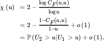
- Transforming Xj to Zj = 1/(1 − Fj(Xj)) (j = 1, 2), which are standard Pareto distributed, P(Zj > z) = z−1, Ledford and Tawn [530] introduced a third dependence coefficient by assuming that the joint survivor function of (Z1, Z2) is regularly varyingwith ℒ a slowly varying function. The extreme value index η of the random variable min(Z1, Z2) is termed the coefficient of tail dependence. Note that
 We find that
- if
 and
and 
- if
 , or
, or  with
with 
 . If 0 < η < 1/2 then we have negative tail dependence.
 - if
As in the univariate case, the domain of attraction condition (3.6.15) can be cast in terms of exceedances over a high threshold. The event ![]() is called an exceedance over the (multivariate) threshold t. This means that there is at least one coordinate variable Xj that exceeds the corresponding threshold tj, although the precise coordinate where this happens remains unspecified. We are then interested in the asymptotic distribution of the excess vector
is called an exceedance over the (multivariate) threshold t. This means that there is at least one coordinate variable Xj that exceeds the corresponding threshold tj, although the precise coordinate where this happens remains unspecified. We are then interested in the asymptotic distribution of the excess vector ![]() conditionally on
conditionally on ![]() , as
, as ![]() . It was shown, for example Beirlant et al. [100] or Rootzén and Tajvidi [654], that if
. It was shown, for example Beirlant et al. [100] or Rootzén and Tajvidi [654], that if ![]() as
as ![]() , and 0 < G(0) < 1,
, and 0 < G(0) < 1,

as ![]() , where
, where ![]() denotes the lower endpoint of Gj. H is then the distribution function of the multivariate generalized Pareto distribution.
denotes the lower endpoint of Gj. H is then the distribution function of the multivariate generalized Pareto distribution.
Based on (3.6.24), (3.6.17) and (3.6.19) we then obtain, when αj > γjμj, j = 1, …, d, that

Setting σj = αj − γjμj and  , we arrive at

for ![]() such that σ + γx > 0. Finally, when x ≥0 we obtain that
such that σ + γx > 0. Finally, when x ≥0 we obtain that

and ![]() (j = 1, …, d). Further note that with properties (L1) and (L2) for STDFs, we obtain in case x ≥0
(j = 1, …, d). Further note that with properties (L1) and (L2) for STDFs, we obtain in case x ≥0

with ![]() . Imposing the constraint l(ζ1, …, ζd) = 1 we then have
. Imposing the constraint l(ζ1, …, ζd) = 1 we then have
For further properties concerning multivariate generalized Pareto distributions see Rootzén and Tajvidi [654] and Kiriliouk et al. [488].