Keywords

Collector; chimney; turbine; helical heat-collecting

4.1 Introduction

Because of the pressure of reducing carbon dioxide emissions, it is becoming more and more urgent for China to carry out various applications and research on new energy generating technologies. The solar chimney power plant system (SC), which has the following advantages while compared with the traditional power generation systems: easier to design, more convenient to draw materials, higher operational reliability, fewer running components, more convenient maintenance and overhaul, lower maintenance expense, no environmental contamination, continuous stable running, longer operational lifespan, was first proposed in the late 1970s by Professor Jörg Schlaich and tested with a prototype model in Manzanares, Spain, in the early 1980s [1,2]. It has the potential to meet the power needs of developing countries and territories, especially in deserts where there is a shortage of electric power, and has extensive application prospects.

Since the SC systems could make significant contributions to the energy supply of those countries where there is plenty of unutilized desert land, in recent years, many researchers have made research reports on this technology and have carried out tracking studies on SC systems. Haaf et al. [1,2] provided fundamental studies for the Spanish prototype in which the energy balance, design criteria, and cost analysis were discussed, and a report on the preliminary test results of the SC system was made. Some small-scale solar chimney devices with power outputs of no more than 10 W were also reported but these could only validate the feasibility and principle of the solar chimney system [3,4].

Different mathematical models based on 1-D thermal equilibrium were advanced by several researchers, Pasumarthi and Sherif [5] developed a mathematical model to study the effects of various environment conditions and geometry on the flow and heat transfer characteristics and output power of the solar chimney. Bernardes et al. [6] established a rounded mathematic model including the collector, chimney, and turbine of an SC system on the basis of the energy-balance principle. Bilgen and Rheault [7] designed a SC system for power production at high latitudes and evaluated its performance. Pretorius and Kröger [8] evaluated the influence of a developed convective heat transfer equation, more accurate turbine inlet loss coefficient, quality collector roof glass, and various types of soil on the performance of a large scale SC system.

Gannon and Von Backström [9] presented an air standard cycle analysis of the SC for the calculation of limiting performance, efficiency, and relationship between main variables including chimney friction, system, turbine, and exit kinetic energy losses. Gannon and Von Backström [10] presented an experimental investigation of the performance of a solar chimney turbine. The measured results showed that the solar chimney turbine presented has a total-to-total efficiency of 85–90% and total-to-static efficiency of 77–80% over the design range. Later, the same authors [11] presented analytical equations in terms of turbine flow and load coefficient and degree of reaction, to express the influence of each coefficient on turbine efficiency. Bernardes et al. [12] developed a thermal and technical analysis to estimate the power output and examine the effect of various ambient conditions and structural dimensions on the power output.

Pastohr et al. [13] carried out a two-dimensional steady-state numerical simulation study on the whole SC system, which consists of the energy storage layer, the collector, the turbine, and the chimney, and obtained the distributions of velocity, pressure, and temperature inside the collector. Ming et al. [14] developed a comprehensive model to evaluate the performance of a SC system, in which the effects of various parameters on the relative static pressure, driving force, power output, and efficiency have been further investigated. Ming et al. [15,16] established different mathematical models for the collector, the chimney, and the energy storage layer and analyzed the effect of solar radiation on the heat storage characteristic of the energy storage layer. Ming et al. [17] carried out numerical simulations on the SC systems coupled with a 3-blade turbine using the Spanish prototype as a practical example and presented the design and simulation of a MW-graded SC system with a 5-blade turbine, the results of which show that the coupling of the turbine increases the maximum power output of the system and the turbine efficiency is also relatively rather high.

The previous research reports indicate that, provided the considerable scale of an SC system, carrying out numerical simulations for it before setting up the commercial system would be an effective method to make predictions of the characteristic parameters and operating characteristics of the system. Apparently, mathematical models based on 1-D thermal equilibrium cannot give detailed descriptions on the temperature, velocity, and pressure distributions of the whole system. During the two-dimension simulation for an SC system carried out by Pastohr et al. [13], the pressure drop across the turbine was preset according to the Beetz power limit theory, as the turbine of the SC system is pressure-based which is similar to the turbine of a hydraulic power station but different from that of a traditional wind power station, therefore, different pressure drops across the turbine can be preset to analyze the power output characteristic of the SC system. In addition, the existing numerical simulation results did not analyze the influences of solar radiation, turbine pressure drop and efficiency on the flow and heat transfer, output power and energy loss of the SC system. Based on this, two-dimension numerical simulations for the Spanish solar chimney power plant prototype, containing an energy storage layer, a collector, a turbine, and the chimney, will be carried out in this paper to analyze the influence of pressure drop across the turbine and solar radiation on items such as flow, heat transfer, energy loss, and power output characteristics of the SC system.

4.2 Theoretical Models

4.2.1 Physics Model

An SC system with the same fundamental dimensions as the Spanish SC prototype will be built in Wuhan, China. Taking the fundamental dimensions of the Spanish SC system shown in Fig. 4.1 as a practical example [2], geometric parameters of the prototype are shown as follows: height of chimney, 200 m; diameter of chimney, 10 m; radius of collector, 122 m; height from the inlet to its center, 2–6 m; thickness of the energy storage layer, 5 m. The collector and the chimney are smoothly connected in order to reduce the energy loss caused by resistance, and in addition a shrink flow passage is designed at the bottom of the collector. The material used for the collector canopy is transparent glass, while the energy storage layer uses the soil that can be regarded as porous media.

4.2.2 Mathematical Model

In natural convection, the strength of the buoyancy-induced flow is measured by the Rayleigh number, defined as follows:

$Ra=\frac{g\beta \mathrm{\Delta }T{L}^3}{a\nu }$ (4.1)

(4.1)

where, $\mathrm{\Delta }T$ is the maximum temperature difference of the system. L, $a$, and $\beta$ are the mean collector height, the thermal diffusivity, and the thermal expansion coefficient, respectively. The whole collector and chimney analysis shows that Ra>10¹⁰, therefore, fluid flow in the regions may be turbulent. Accordingly, the axisymmetric mathematical model including the continuity equation, Navier-Stocks equation, energy equation, and $\kappa -\epsilon$ equations used to describe the problem are as follows:

$\frac{\partial (\rho u)}{\partial x}+\frac{1}{r}\frac{\partial (r\rho v)}{\partial r}=0$ (4.2)

(4.2)

$\begin{array}{l}\frac{\partial }{\partial x}(\rho uu)+\frac{1}{r}\frac{\partial }{\partial r}(r\rho vu)=\frac{\partial }{\partial x}\left((\mu +{\mu }_t)\frac{\partial u}{\partial x}\right)+\frac{1}{r}\frac{\partial }{\partial r}\left((\mu +{\mu }_t)r\frac{\partial u}{\partial r}\right)\hfill \\ +\rho g\beta (T-T_0)+\frac{\partial }{\partial x}\left((\mu +{\mu }_t)\frac{\partial u}{\partial x}\right)+\frac{1}{r}\frac{\partial }{\partial r}\left((\mu +{\mu }_t)r\frac{\partial v}{\partial x}\right)\hfill \end{array}$ (4.3)

(4.3)

$\begin{array}{l}\frac{\partial }{\partial x}(\rho uv)+\frac{1}{r}\frac{\partial }{\partial r}(r\rho vv)=\frac{\partial }{\partial x}\left((\mu +{\mu }_t)\frac{\partial v}{\partial x}\right)+\frac{1}{r}\frac{\partial }{\partial r}\left((\mu +{\mu }_t)r\frac{\partial v}{\partial r}\right)\\ +-\frac{\partial p}{\partial r}+\frac{\partial }{\partial x}\left((\mu +{\mu }_t)\frac{\partial u}{\partial r}\right)+\frac{1}{r}\frac{\partial }{\partial r}\left((\mu +{\mu }_t)r\frac{\partial v}{\partial r}\right)-\frac{2(\mu +{\mu }_t)v}{r^2}\end{array}$ (4.4)

(4.4)

$\frac{\partial (uT)}{\partial x}+\frac{1}{r}\frac{\partial (rvT)}{\partial r}=\frac{1}{\rho }\frac{\partial }{\partial x}\left(\left(\frac{\mu }{\mathrm{Pr}}+\frac{{\mu }_t}{{\sigma }_T}\right)\frac{\partial T}{\partial x}\right)+\frac{1}{\rho r}\frac{\partial }{\partial r}\left(\left(\frac{\mu }{\mathrm{Pr}}+\frac{{\mu }_t}{{\sigma }_T}\right)r\frac{\partial T}{\partial r}\right)$ (4.5)

(4.5)

$\frac{\partial (u\kappa )}{\partial x}+\frac{1}{r}\frac{\partial (rv\kappa )}{\partial r}=\frac{1}{\rho }\frac{\partial }{\partial x}\left(\left(\mu +\frac{{\mu }_t}{{\sigma }_{\kappa }}\right)\frac{\partial \kappa }{\partial x}\right)+\frac{1}{\rho r}\frac{\partial }{\partial r}\left(\left(\mu +\frac{{\mu }_t}{{\sigma }_{\kappa }}\right)r\frac{\partial \kappa }{\partial r}\right)+G_{\kappa }-\epsilon$ (4.6)

(4.6)

$\frac{\partial (u\epsilon )}{\partial x}+\frac{1}{r}\frac{\partial (rv\epsilon )}{\partial r}=\frac{1}{\rho }\frac{\partial }{\partial x}\left(\left(\mu +\frac{{\mu }_t}{{\sigma }_{\epsilon }}\right)\frac{\partial \epsilon }{\partial x}\right)+\frac{1}{\rho r}\frac{\partial }{\partial r}\left(\left(\mu +\frac{{\mu }_t}{{\sigma }_{\epsilon }}\right)r\frac{\partial \epsilon }{\partial r}\right)+\frac{\epsilon }{\kappa }\left(C_1{G}_{\kappa }-C_2\epsilon \right)$ (4.7)

(4.7)

where, $G_{\kappa }$ represents the generation of turbulence kinetic energy due to the mean velocity gradients defined as: $G_{\kappa }=-{\mu }_t\left(2\left({\left(\frac{\partial u}{\partial x}\right)}^2+{\left(\frac{\partial v}{\partial r}\right)}^2+{\left(\frac{v}{r}\right)}^2\right)+{\left(\frac{\partial u}{\partial r}+\frac{\partial v}{\partial x}\right)}^2\right)$. ${\sigma }_T$,${\sigma }_{\kappa }$, and ${\sigma }_{\epsilon }$ are the turbulent Prandtl numbers for T, $\kappa$, and $\epsilon$, respectively, and $c_1$ and $c_2$ are two constants for the turbulent model: $c_1=1.44$,$c_2=1.92$,${\sigma }_T=0.9$, ${\sigma }_{\kappa }=1.0$,${\sigma }_{\epsilon }=1.3$.${\mu }_t=\frac{c_{\mu }\rho {\kappa }^2}{\epsilon }$, and $c_{\mu }=0.09$.

The heat transfer and flow in the energy storage layer may be very complicated, and it is necessary to take into account the collector, the chimney, and the storage medium as a whole system. As the material used for the energy storage layer can be regarded as a porous medium, the Brinkman–Forchheimer Extended Darcy model [18] is used to describe the flow in the convective porous-layer, which can be expressed as follows:

$\frac{\partial u}{\partial x}+\frac{1}{r}\frac{\partial (rv)}{\partial r}=0$ (4.8)

(4.8)

$\begin{array}{l}\frac{\rho }{\phi }\frac{\partial u}{\partial t}+\frac{\rho }{{\phi }^2}\left(\frac{\partial (uu)}{\partial x}+\frac{1}{r}\frac{\partial (rvu)}{\partial r}\right)=-\frac{\partial p}{\partial x}+\frac{\partial }{\partial x}\left({\mu }_m\frac{\partial u}{\partial x}\right)\\ +\frac{1}{r}\frac{\partial }{\partial r}\left(r{\mu }_m\frac{\partial u}{\partial r}\right)-\frac{\mu u}{K}-\frac{\rho F}{\sqrt{K}}\sqrt{u^2+v^2}u+\rho g\beta \left(T-T_e\right)\end{array}$ (4.9)

(4.9)

$\begin{array}{c}\frac{\rho }{\phi }\frac{\partial v}{\partial t}+\frac{\rho }{{\phi }^2}\left(\frac{\partial (uv)}{\partial z}+\frac{1}{r}\frac{\partial (rvv)}{\partial r}\right)=\frac{\partial }{\partial z}\left({\mu }_m\frac{\partial v}{\partial z}\right)+\\ \frac{1}{r}\frac{\partial }{\partial r}\left(r{\mu }_m\frac{\partial v}{\partial r}\right)-{\mu }_m\frac{v}{r^2}-\frac{\mu u}{K}-\frac{\rho F}{\sqrt{K}}\sqrt{u^2+v^2}v\end{array}$ (4.10)

(4.10)

${\rho }_m{c}_{p,m}\left(\frac{\partial T}{\partial t}+\frac{\partial (uT)}{\partial z}+\frac{1}{r}\frac{\partial (rvT)}{\partial r}\right)=\frac{\partial }{\partial z}\left({\lambda }_m\frac{\partial T}{\partial z}\right)+\frac{1}{r}\frac{\partial }{\partial r}\left(r{\lambda }_m\frac{\partial T}{\partial r}\right)$ (4.11)

(4.11)

where, $\phi$, ${\rho }_m$, $c_{p,m}$, ${\mu }_m$, and ${\lambda }_m$ are the porosity, apparent density, specific capacity, dynamic viscosity, and apparent thermal conductivity of the porous medium, respectively: ${\rho }_m=(1-\phi ){\rho }_s+\phi {\rho }_a$, $c_{p,m}=(1-\phi )c_{p,s}+\phi c_{p,a}$, ${\lambda }_m=(1-\phi ){\lambda }_s+\phi {\lambda }_a$, ${\mu }_m=\mu /\phi$; the parameters with subscripts s and a denote the corresponding parameters of the solid and air in the energy storage layer, respectively. $K$, F, and $d_b$ are the permeability, the inertia coefficient, and the particle diameter of the energy storage layer, respectively.

$K={d_b}^2{\phi }^3/(175{(1-\phi )}^2)$ (4.12)

(4.12)

$F=1.75{\phi }^{-1.5}/\sqrt{175}$ (4.13)

(4.13)

4.2.3 Boundary Conditions and Solution Method

Boundary conditions are set as follows: For the roof of the collector, we take the convection boundary into account, and the coefficient of convection is set as 10 W/(m² K) which can be accepted when the environment air velocity is not very large, that is, 1~2 m/s. The temperature of the environment is set as 293K; the inlet of the collector is set as the pressure-inlet boundary; the chimney wall can be set as an adiabatic boundary; the chimney outlet is set as the pressure-outlet boundary; the bottom of the energy storage layer is set as the temperature-constant boundary, whose temperature is 300K. Solar radiation which projects through the transparent ceiling into the ground can be considered as a heat source for the ground thin layer [13]. In recent years, the highest solar radiation in Wuhan area is about 650 W, therefore, we can simulate the running conditions of a SC system in Wuhan on the whole by setting solar radiation as 200, 400, 600, and 800 W/m², respectively.

In addition, it is necessary to explain the reason why we consider the collector inlet and chimney outlet both as pressure boundaries and have their pressures set as 0 Pa. This is because we simultaneously take the inner and outer pressure distributions of the system into account [13]; $p_{r,i}=0$ means that for both the inside and outside of the collector inlet, the static pressures at the same height are the same.

However, the setting of the pressure drop across the turbine in this paper differs from the processing method applied by Pastohr [13]. The turbine of an SC system, as explained earlier, belongs to a pressure-based wind turbine, the fore-and-aft air velocities are almost the same but the pressure changes significantly, and its power output does not follow the Beetz power limit theory. Thereby the output power through the turbine can be calculated according to Eq. (4.14) by presetting the pressure drop across the turbine:

$W_t={\eta }_t·\mathrm{\Delta }p·V$ (4.14)

(4.14)

where, $W_t$ represents the shaft power output through the turbine, ${\eta }_t$ represents the energy conversion efficiency of the turbine, which can be preset as 80%, less than the optimized data [10,11], $\mathrm{\Delta }p$ represents the pressure drop across the turbine, V represents the air volume flow rate of the system flowing through the chimney outlet. The boundary conditions for different locations are shown in Table 4.1.

Table 4.1

Boundary Conditions

Location	Type	Value
0.1 mm top layer of the ground	Heat source	2×106~8×106 W/m3
Bottom of the ground	Temperature	300K
Surface of the canopy	Wall	Te=293K, h=10 W/(m2·K)
Surface of the chimney	Wall	qchim=0 W/m2
Collector inlet	Pressure inlet	pr,i=0 Pa, T0=293K
Chimney outlet	Pressure outlet	pr,o=0 Pa
Pressure drop across the turbine	Reverse fan	0~480 Pa, 40 Pa in interval

The standard $k-\epsilon$ model is applied during the numerical simulation of air flow in the collector and chimney, The material for the energy storage layer is selected as soil, and the properties of the soil are as follows: ρ_soil=1700 kg/m³, c_p,_soil=2016 J/(kg·K), λ_soil=0.78 W/(m·K). The porosity of the energy storage layer is selected as 0.1, as in Wuhan, China, the soil is almost close-grained. The standard wall function method is applied, the SIMPLE algorithm is applied for pressure-velocity coupling, and the momentum equation, energy equation, and other equations all apply the second-order upwind discretization scheme. The mesh number of the SC system is nearly 500,000, where we can get a grid-independent simulation result. In addition, the feasibility of this numerical method can be found in Ref. [15].

4.3 Results and Discussion

Currently, solar power plant and wind power plant are the main power generation systems using renewable energy, namely solar power and wind power respectively. Turbines applied in an SC system and a wind power plant are pressure-based impulse turbines and velocity-based impulse turbines, respectively. For the former system, where the air flow is subjected to the area of the chimney, fore-and-aft velocity changes little, accompanied with a pressure drop. In the latter system, fore-and-aft pressure changes little while the velocity decreases significantly.

Figs. 4.2–4.4 show the simulation results on flow and heat transfer characteristics of the SC system when solar radiation and pressure drop across the turbine are 400 W/m² and 0 Pa (when turbine is not in service), respectively. As shown in Fig. 4.2, relative static pressure (defined as the difference between the inner-system static pressure and the environment static pressure at the same height) inside the system has negative values everywhere, this indicates that pressure inside the system is always lower than that of the environment. Among this, the pressure difference between the chimney bottom and the environment comes to the maximum. Meanwhile, the velocity also reaches its maximum which is over 12 m/s. On the other hand, temperature inside the system increases up to 307K, experiencing a 15K change compared with the environment temperature. Obviously, under no-load condition, this temperature variation is not very dramatic.

Figs. 4.5–4.8 show the simulation results on flow and heat transfer characteristics of the SC system when solar radiation and pressure drop across the turbine are 400 W/m² and 120 Pa, respectively. It is found that, compared with Figs. 4.5–4.6 and 4.2, the pressure distribution inside the system has experienced dramatic variations, among which the pressure drop within the turbine area is extremely dramatic. This is because the turbine is preset a 120 Pa pressure drop during this numerical simulation, and the results as shown in Figs. 4.5 and 4.6 exactly reflect this effect.

Through comparing the two simulation results corresponding to the turbine pressure drops being 0 and 120 Pa respectively, we found that when the turbine pressure drop increases, the inside-outside pressure difference of the system increases, velocity of the air flow decreases, while the temperature of the air flow increases, for which the main reason is that the turbine pressure drop has an inverse effect on the air velocity. Thus the heating-up period is prolonged, and the temperature at the chimney outlet increases with the pressure drop across the turbine.

Figs. 4.9 and 4.10 show the influences of solar radiation and turbine pressure drop on the temperature and velocity at the chimney outlet. As shown in the figures, when the turbine pressure drop increases, the chimney outlet temperature increases, while the chimney outlet velocity decreases gradually. This is because the increase of turbine pressure drop causes a block effect to the air flow within the system which makes the air flow rate of the system decrease. As a result, the heating-up time of the air inside the collector is prolonged and the chimney outlet temperature increases. Meanwhile, if the turbine pressure drop keeps constant, the air velocity increases notably with the solar radiation, which originates from the relatively high extent to which the fluid is heated during free convection process. Therefore, both the temperature and velocity of the chimney outlet increase.

In general, the air velocities before turbines are often in the scope of 8–9 m/s when wind turbines are in their operation conditions. Based on this scope, it is shown from Fig. 4.10, corresponding to solar radiation being 200, 400, 600, and 800 W/m², respectively, that the optimal values of the turbine pressure drop are 40, 120, 200, and 280 Pa, respectively. As shown in Fig. 4.9, the variation range for the chimney outlet temperature is 303~333K under four optimal turbine pressure drops, and the chimney outlet temperature is 320K when the solar radiation and turbine pressure drop are 600 W/m² and 200 Pa, respectively.

Fig. 4.11 shows the influences of the turbine pressure drop and solar radiation on the turbine output power of the SC system, in which the efficiency of turbine is preset as 80%. As shown in Fig. 4.11, if the turbine pressure drop keeps constant, output power of the system increases with the solar radiation. This is because the increase of solar radiation will result in a notable increase of the system air volume flow rate. However, the influence of turbine pressure drop on the system output power is rather complicated. Under a small turbine pressure drop, the system output power increases with the turbine pressure drop. According to Eq. (4.14), the main reason for this phenomenon is that the reduction of the air volume flow rate of the system caused by the turbine pressure drop is relatively small, making the product of the air volume flow rate and the pressure drop across the turbine present a rise trend. But when the turbine pressure drop is fairly large, the air volume flow rate decreases more significantly than the extent to which the turbine pressure drop increases, thus resulting in a reduction of the system output power.

Through comparing the simulation results in Fig. 4.11 and the experimental results of the Spanish SC prototype system [2], we found that the experimental output power of the Spanish SC prototype system is 35 kW under a solar radiation of about 750 W/m², while the maximum output power in Fig. 4.11 is higher than 40 kW under a solar radiation of only 200 W/m². The main reason for this difference is that the design of the turbine used in the Spanish SC prototype system is far from optimization. From Fig. 4.11 we can see that the output power of the system by using an optimized turbine will be much higher than that of the Spanish SC prototype system when the solar radiation is over 600 W/m². However, no system output power was reported in Ref. [13] which based its simulation for turbine operation on Beetz theory during the simulation process. On the other hand, as mentioned above, the power efficiency of a pressure-based turbine dramatically differs from that of a velocity-based free wind field turbine. The simulation results in this work take the turbine as pressure-based, and the turbine efficiency is preset as 80% which is fairly easy to achieve, as shown in Refs. [10,11], as a result, this brings about relatively a dramatic difference between the theoretical simulation results and the experimental results shown in Ref. [2], which serves as a theoretical law for further optimum design of the turbine coupled with the SC system.

Fig. 4.12 shows the influences of turbine efficiency and turbine pressure drop on the system output power under a solar radiation of 600 W/m². As shown in this figure, besides the notable influence of turbine pressure drop on the output power of the system, the turbine efficiency also has a notable influence on the output power of the system. With the turbine pressure drop remaining constant, the higher the efficiency of turbine, the larger the output power of the system. Again through comparing the simulation results in this work with the experimental results in Ref. [2], we found that even if the turbine efficiency is only 50%, provided that that solar radiation is 600 W/m² and pressure drop is in the scope of 80~400 Pa, the system output power is always larger than the experimental results shown in Ref. [2]. Therefore, it is concluded that if we increase the turbine efficiency by improving the turbine structure to an optimized design, the system output power will increase remarkably. Additionally, Fig. 4.12 also indicates that the pressure-based turbine of the SC system is able to run in a relatively wide range of turbine pressure drop with a fairly large system output power.

According to the simulation results as shown in Fig. 4.11, under a solar radiation of 600 W/m², the system output power is merely 120 kW, even when an ideal and optimum designed turbine with a turbine efficiency of 80% is applied. Taking the fact that the component which receives solar radiation within the system is a collector whose radius is 122 m, we can concluded that the total energy conversion efficiency from solar energy to turbine shaft output power is only 0.428%, for which the main reason is possibly excessive energy loss.

When the air flows through the chimney outlet, the total energy loss includes kinetic energy loss, gravitational potential energy, and enthalpy, among which the fractional of the kinetic energy and gravitational potential energy are far smaller than the air enthalpy flowing out of the system. These two items of macroscopic energy loss are negligible when calculating energy loss from chimney outlet. Therefore the total energy loss from the chimney outlet can be defined as the total enthalpy difference between the chimney outlet and the collector inlet. Fig. 4.13 shows the influence of turbine pressure drop and solar radiation on energy loss from the chimney outlet. As shown in this figure, energy loss from the chimney outlet is obviously rather large, it is 100–1000 times larger than the output power of the system. It indicates that the chimney outlet becomes the most important part of energy loss from the system. When the pressure drop across the turbine is small, the total energy loss from the chimney outlet accounts for 90% of the solar energy received by the system; even when the turbine pressure drop is high, the energy loss from the chimney outlet still accounts for about 75% of total solar energy received by the system, thus resulting in a rather low energy conversion efficiency of the system. Furthermore, from Fig. 4.13 we can also see that energy loss from the chimney outlet increases significantly with the solar radiation but decreases with the turbine pressure drop which is mainly because the air flow rate decreases dramatically with the turbine pressure drop.

Fig. 4.14 shows the energy loss from the canopy caused by the turbine pressure drop and the solar radiation. Obviously, energy loss from the canopy increases significantly with pressure drop across the turbine. Under a solar radiation of 200 W/m² and a pressure drop across the turbine of 200 Pa, the total energy loss from the canopy is nearly 2 MW, namely 50 W/m² from the system to the environment through the canopy, which is nearly 1/4 of the solar radiation intensity; under a solar radiation intensity of 600 W/m² and a pressure drop across the turbine of 360 Pa, the total energy loss from the canopy is as much as 5 MW, namely 125 W/m², which is also nearly 1/4 of total solar radiation received. These numbers illustrate that the energy loss from the canopy is also very large, and one way to reduce energy loss from the canopy is to apply a double-layer transparent material, which can effectively reduce energy loss from the canopy.

In addition, numerical simulation results show that the portion of energy loss toward the ground through the energy storage layer is rather small, and is far smaller than the portion of energy loss through the chimney outlet and canopy. When the solar radiation and turbine pressure drop are 600 W/m² and 360 Pa, respectively, the total energy loss from the bottom of the energy storage layer is only 600 kW. Therefore, the energy loss through the bottom of the energy storage layer is negligible when analyzing the total energy loss of SC system.

4.4 Helical Heat-Collecting Solar Chimney Power Plant System

As for SC systems that already have certain scale, elements that determine the initial investment include: chimney, collector, turbine, etc. In detail, the chimney decides the system’s efficiency, decreasing the chimney’s height will remarkably reduce the cost of SC system but also decrease the system’s efficiency. Therefore, choosing cheap materials or applying the Floating Solar chimney [19–22] is feasible in reducing the cost of the chimney. Increasing the turbine’s efficiency is also another important method in reducing the cost of SC system, which is the main focus for a lot of research being undertaken [10,11,23]. Concerning the fact that the area of the collector is rather large, when the system material is selected, the cost of the collector and SC system’s power increase as the area of the collector increases, considering the cost of land area and material, the area of the collector has a determinant influence on the economical efficiency of the whole system. If the area of the collector is shrunk in a proper manner while the maximum system output power remains the same under the same solar radiation, then the efficiency of the SC system can be increased, the system’s economical efficiency of the system is improved, while the initial investment is reduced. In this chapter, a new type of helical heat-collecting solar chimney power generating system is proposed, and numerical analysis on the system’s fluid flow and heat transfer characteristics is carried out and compared with the experimental and simulation results of the solar chimney prototype plant in Spain.

4.5 Mathematical and Physical Model

4.5.1 Physical Model

The basic dimensions of the SC prototype plant in Spain are as follows: chimney height, 200 m; chimney radius, 10 m; collector radius, 122 m; height between the inlet of the collector and the center, 2~6 m. In order to compare the helical heat-collecting SC system with the SC prototype plant in Spain [1], the basic dimensions of the helical heat-collecting SC system established in this paper are as follows: chimney height, 200 m; chimney diameter, 10 m; collector radius, 90 m; height between the inlet of the collector and the center, 2~6 m. The planform of the system is shown as Fig. 4.15, 4 helical transparent walls, which can be made of the same glass material as the canopy of the collector, are set in the center—the reason for applying transparent glass as the wall material is to avoid the shading of solar radiation. Through design, the fluid is driven to flow along the helical transparent wall to the collector center, hence the actual route length along which the fluid is heated within the collector is 145 m. In order to reduce the resistance loss, the collector and the chimney are smoothly connected; moreover, shrinkage flow path is applied at the collector bottom. The canopy of the collector is made of transparent glass.

4.5.2 Mathematical Model

Through analysis, the fluid flow within the collector and the chimney should be a vigorous turbulence region. The relevant continuity equations, N-S equations, energy equations, and turbulence equations are as follows:

$\frac{\partial \rho }{\partial t}+\frac{\partial (\rho u)}{\partial x}+\frac{\partial (\rho v)}{\partial y}+\frac{\partial (\rho w)}{\partial z}=0$ (4.15)

(4.15)

$\frac{\partial (\rho u)}{\partial t}+\frac{\partial (\rho uu)}{\partial x}+\frac{\partial (\rho vu)}{\partial y}+\frac{\partial (\rho wu)}{\partial z}=\rho g\beta (T-T_{\infty })+\mu \left(\frac{{\partial }^{2}u}{\partial x^2}+\frac{{\partial }^{2}u}{\partial y^2}+\frac{{\partial }^{2}u}{\partial z^2}\right)$ (4.16)

(4.16)

$\frac{\partial (\rho v)}{\partial t}+\frac{\partial (\rho uv)}{\partial x}+\frac{\partial (\rho vv)}{\partial y}+\frac{\partial (\rho wv)}{\partial z}=-\frac{\partial p}{\partial y}+\mu \left(\frac{{\partial }^{2}v}{\partial x^2}+\frac{{\partial }^{2}v}{\partial y^2}+\frac{{\partial }^{2}v}{\partial z^2}\right)$ (4.17)

(4.17)

$\frac{\partial (\rho w)}{\partial t}+\frac{\partial (\rho uw)}{\partial x}+\frac{\partial (\rho vw)}{\partial y}+\frac{\partial (\rho ww)}{\partial z}=-\frac{\partial p}{\partial z}+\mu \left(\frac{{\partial }^{2}w}{\partial x^2}+\frac{{\partial }^{2}w}{\partial y^2}+\frac{{\partial }^{2}w}{\partial z^2}\right)$ (4.18)

(4.18)

$\frac{\partial (\rho cT)}{\partial t}+\frac{\partial (\rho cuT)}{\partial x}+\frac{\partial (\rho cvT)}{\partial y}+\frac{\partial (\rho cwT)}{\partial z}=\lambda \left(\frac{{\partial }^{2}T}{\partial x^2}+\frac{{\partial }^{2}T}{\partial y^2}+\frac{{\partial }^{2}T}{\partial z^2}\right)$ (4.19)

(4.19)

$\frac{\partial }{\partial t}\left(\rho k\right)+\frac{\partial }{\partial x_i}\left(\rho k{u}_i\right)=\frac{\partial }{\partial x_j}\left(\left(\mu +\frac{{\mu }_t}{{\sigma }_k}\right)\frac{\partial k}{\partial x_j}\right)+G_k+G_b-\rho \epsilon +S_k$ (4.20)

(4.20)

$\frac{\partial }{\partial t}\left(\rho \epsilon \right)+\frac{\partial }{\partial x_i}\left(\rho \epsilon u_i\right)=\frac{\partial }{\partial x_j}\left(\left(\mu +\frac{{\mu }_t}{{\sigma }_{\epsilon }}\right)\frac{\partial \epsilon }{\partial x_j}\right)+C_{1\epsilon }(G_k+C_{3\epsilon }{G}_b)-C_{2\epsilon }\rho \frac{{\epsilon }^2}{k}+S_{\epsilon }$ (4.21)

(4.21)

In the equations above, $G_k$ represents the turbulence kinetic energy generation item caused by average velocity gradient: $G_k=-\rho \overline{{u\prime }_i{u\prime }_j}\frac{\partial u_j}{\partial x_i}$; $G_b$ refers to the turbulence kinetic energy generation item caused by buoyancy; ${\sigma }_k$ and ${\sigma }_{\epsilon }$ are constants of $k-\epsilon$ equations; $\beta$ refers to the coefficient of cubic expansion: $\beta \approx 1/T$.

4.5.3 Solving Determinant Condition and Solution

1. Heat balance condition of the glass surface of the collector canopy

$Q_{g,air}+Q_{g,e}+Q_{g,stor}+Q_{g,sky}+\alpha Q_{solar}=0$ (4.22)

(4.22)

In the equation above, $Q_{g,air}$ refers to the heat convection flux between the collector surface and air inside the collector. As the temperature difference between them is not big at all, hence the radiation heat transfer between them is negligible. $Q_{g,air}=A_g{h}_{g,air}\left(T_g-T_a\right)$, where $A_g$ refers to the surface of the collector; $h_{g,air}$ refers to the convection heat transfer coefficient between the collector surface and the air inside the collector; $T_g$ and $T_a$ represent the thermodynamic temperature of the collector surface and the air inside the collector, respectively; $Q_{g,e}$ refers to the convection heat transfer flux between the collector surface and the ambient air, $Q_{g,e}=A_g{h}_{g,e}\left(T_g-T_e\right)$; $h_{g,e}$ refers to the convection heat transfer coefficient between the collector surface and the ambient air; $T_e$ refers to the thermodynamic temperature of the ambient air; $Q_{g,stor}$ refers to the radiation heat transfer flux between the collector surface and the surface of the heat storage layer at the bottom of the collector, Considering the radiation heat transfer between the collector surface and the heat storage layer as radiation heat transfer between two parallel plates of the same area and ignoring the radiation loss at the collector inlet and outlet, we have: $Q_{g,stor}=A_g\sigma \left({T_g}^4-{T_{stor}}^4\right)$, where $\sigma$ refers to Stephen Boltzmann constant; $T_{stor}$ refers to the thermodynamic temperature of the heat storage layer; $Q_{g,sky}$ refers to the radiation heat transfer flux between the collector surface and the sky, $Q_{g,sky}=A_g\sigma \left({T_g}^4-{T_{sky}}^4\right)$; $Q_{solar}$ refers to the solar radiation received by the collector; $\alpha$ refers to the absorptivity of the transparent material of the collector.

2. Surface condition of heat storage layer

$Q_{stor,air}+Q_{stor,g}+Q_{stor,down}+\eta \tau Q_{solar}=0$ (4.23)

(4.23)

$Q_{stor,air}$ refers to the heat transfer flux between the heat storage layer and the air inside the collector, $Q_{stor,air}=A_{stor}{h}_{stor,air}\left(T_{stor}-T_{air}\right)$; $A_{stor}$ refers to the heat transfer area of the heat storage layer: $A_{stor}=A_g$; $h_{stor,air}$ refers to the convection heat transfer coefficient between the heat storage layer surface and the air inside the collector; $Q_{stor,g}$ refers to the radiation heat transfer flux between the heat storage layer surface and the collector surface, according to the analysis above, we have the equation as follows: $Q_{stor,g}=-Q_{g,stor}=A_g\sigma \left({T_{stor}}^4-{T_g}^4\right)$. $Q_{stor,down}$ refers to the heat transfer flux from the heat storage layer surface to the heat storage layer: $Q_{stor,down}=-A_{stor}{\lambda }_{stor}\frac{dT}{dx}$, in which ${\lambda }_{stor}$ refers to the heat conductivity of the heat storage layer. $\tau$ refers to the collector material’s solar radiation transmissivity; $\eta$ refers to the heat storage layer surface’s solar radiation absorptivity.

3. Balance conditions for chimney surface
As taking the heat dissipation from chimney to the ambience into account will make the simulation more practical, the third boundary condition is set as follows:

$-\lambda {\left(\frac{\partial t}{\partial y}\right)}_w=h\left(T_w-T_{enviro}\right)$ (4.24)

(4.24)

In the equation above, the convection heat transfer coefficient is as follows: $h=5.7+3.8V_{enviro}$, where $V_{enviro}$ refers to the ambient wind velocity, and $T_{enviro}$ refer to the ambient temperature. However, considering the facts that the heat convection area is far smaller than that of the collector canopy and the chimney wall is rather thick, it can be considered as adiabatic.

4. Conditions for collector inlet
In accordance with Refs. [13,14], it is assumed that the pressure at the collector inlet is the same as the ambience, hence the collector inlet pressure condition can be set as follows:

$p_{r,inlet}=0$ (4.25)

(4.25)

The $k-\epsilon$ model is applied for the fluid flow within the system, the standard wall function is applied for wall processing, the SIMPLE algorithm is applied for pressure-velocity coupling, and the QUICK format is applied for equations including momentum equation, energy equation, and other equations. When the mesh number exceeds 120 million, the computation results is grid-independent.

4.6 Validition

Comparison between the numerical simulation results and the experimental results collected on Sep. 2, 1982 of the Spanish SC system is now carried out in order to verify the validity of the numerical simulation results in this chapter. The computation parameters are set according to literature [2], and solar radiation and ambient parameters are set as key conditions for the numerical simulation. As indicated in Fig. 4.16, the simulation results are quite consistent with the experimental results. In detail, the simulation results fluctuate slightly but its curve is relatively quite smooth. Moreover, its difference from the experimental results is less than 5%. The simulation results are slightly higher than experimental results at noon, which is because the ambient wind velocity was not measured, whereas when we consider the collector canopy’s heat dissipation we assume that the ambient wind velocity is just 2 m/s, which may have underestimated the heat dissipation from the system to the ambience. Hence it can be concluded that the numerical simulation method applied in this paper is effective and feasible.

4.7 Computation Results and Analysis

4.7.1 Comparison on Flow and Heat Transfer Characteristics

Fig. 4.17 shows the comparison of relative static pressure distributions between the Spanish SC prototype plant and the helical heat-collecting SC system. As shown in this figure, the relative static pressure distribution within the chimney of the new type SC system experiences remarkable variations after applying the helical heat-collecting structure for the collector. The biggest relative static pressure difference at the chimney bottom between the two models is about 15 Pa, which illustrates that the Spanish SC prototype plant is a bit higher than helical heat-collecting SC system. But on the other hand, at a height of 20 m of the chimney, the relative static pressures of Spanish SC prototype plant and helical heat-collecting SC system are −109 and −86 Pa, respectively, which illustrates that the pressure variation within the helical heat-collecting SC system is more remarkable. As the turbine of the SC system is pressure based, the bigger the pressure variation within the SC system, the bigger the pressure head provided for the turbine. Therefore, as shown in Fig. 4.17b, the helical heat-collecting SC system is able to provide the wind turbine with a bigger pressure head, which is positive for the improvement of the generation power output and the energy conversion efficiency of the whole SC system.

Fig. 4.18 shows the comparison of velocity distributions between the Spanish SC prototype plant and the helical heat-collecting SC system. It can be seen from this figure that the velocity distributions inside the chimney of the two types of models are rather close to each other in despite of slight differences. At the same height of the chimney, the velocity of the Spanish SC prototype plant is a little higher than that of the helical heat-collecting SC system, for which the two main reasons are as follows: firstly, the collector radius of the helical heat-collecting SC system is only 90 m, which obviously is smaller than that of the Spanish SC prototype plant (122 m); secondly, although applying the helical heat-collecting type drives the fluid to flow in a helical route toward the chimney and the actual length of flow accordingly reaches 145 m, the helical flow direction keeps changing all the way resulting in an increase of the fluid flow resistance, which not only decreases the fluid flow velocity but also decreases the pressure head used for turbine generating within the system. Therefore, it is necessary to take flow resistance into account and avoid its excessive increase when designing the helical heat-collecting walls.

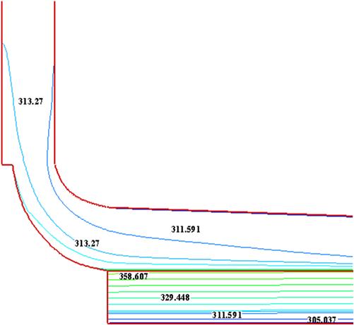
Fig. 4.19 shows the comparison of temperature distributions between the Spanish SC prototype plant and helical heat-collecting SC system. As shown, the temperature distributions of the two types of models at the same height of the chimney are also very close to each other, which illustrates that the heat absorbed by the fluid during the flow and the according temperature rise of the helical heat-collecting SC system are both close to the Spanish SC prototype plant. Nevertheless, it is found through further observance that the temperature distributions within the collector of the two systems are remarkably different from each other, for which the reason is that the fluid flow direction within the helical heat-collecting SC system is not radial but helical, hence the temperature step change shown within the collector is mainly a result of the difference of the channel of fluid flow.

4.7.2 Comparison of Output Power for the Two Type of Models

For further comparison on output power and generating characteristics between the two types of models, the output power under different solar radiations and turbine pressure drops based upon the above mentioned two models are examined. The turbine of SC system is pressure-based, the turbine efficiency is set as 72%, and the output power is the product of the system volume flow, turbine pressure drop, and the turbine efficiency. Fig. 4.20 shows the output power computation results comparison between the Spanish SC prototype plant and the helical heat-collecting SC system, herein G refers to the solar radiation. As shown in the figure, the output powers of the two models are very close to each other under the same solar radiation and turbine pressure drop, and the biggest deviation is less than 3%. Thus, it can be concluded that the helical heat-collecting SC system is of better economical efficiency and bigger commercial advantage when compared with the traditional SC system.

Attention must be paid to the fact that it is not necessary to compare the numerical simulation results with the experimental results of the Spanish SC prototype plant, as the turbine efficiency of the Spanish SC prototype plant was not well designed or optimized. The efficiencies of new turbines specially designed for SC systems have all surpassed 72% [10,11,23], therefore, it is reasonable to set 72% as the turbine efficiency while comparing the numerical results of the two types of SC plants.

4.7.3 Comparison of Different Helical-Wall SC Systems

Figs. 4.21 and 4.22 shows different models of helical-wall SC systems and the corresponding output powers when the solar radiation is 600 W/m². From Fig. 4.22 we can see that the number of helical walls have a significant influence on the output power of the SC system. With the same turbine pressure drop, the output powers of system with 4 helical walls are a little higher than that of systems without helical wall, whereas the output powers of systems with 2 helical walls are a little lower than that of systems without helical walls. This is because the helical fluid flow inside the collector does not form if the system has less than 4 helical walls. Furthermore, in the A and B regions shown in Fig. 4.21a, it is due to the existence of the 2 helical walls of the system that the fluid flow through the chimney is blocked and the output power decreases. As is shown in Fig. 4.22, when the SC system has 6 helical walls or more, the output power increases greatly, the helical fluid flow forms, and the system will operate in a good condition. Apparently, setting up 8 helical walls to this small SC system is the optimal selection.

4.8 Conclusion

Two-dimensional steady-state numerical simulations for the solar chimney power plant system, which includes collector, chimney, turbine, and energy storage layer, are carried out in this paper. The turbine is regarded as a pressure-based one which is different from that in Ref. [13] and the energy storage layer is treated as a porous media, as mentioned in Ref. [15], aiming to analyze the pressure, velocity, and temperature distributions of the system. Meanwhile, the influence of the turbine pressure drop on the flow and heat transfer characteristics and the output power of the SC system are considered. The influences of solar radiation and turbine efficiency on the output power and energy loss of the system are also analyzed. Through analysis, it is found that the influences of solar radiation and pressure drop across the turbine are rather considerable; large outflow of heated fluid from the chimney outlet becomes the main cause for the energy loss of the system, and the canopy also causes considerable energy loss.

A new type of helical heat-collecting SC system has been designed. Through numerical simulation on its flow and heat transfer characteristics, it is found that, considering the fact that the collector radius of the helical heat-collecting SC system is just 90 m, the new model’s radius is decreased by 25%, while its land area and materials are decreased by about 33~43% when compared with the Spanish SC prototype plant. The differences of fluid flow and heat transfer characteristic parameters between the Spanish SC prototype plant and the 8-helical-wall heat-collecting SC system are slight. Therefore, it can be concluded that helical heat-collecting SC system is of better economical efficiency and bigger commercial advantage than the traditional SC system, especially when we take the initial investment into account.

Nomenclature

$u$ Average velocity magnitude in the axial direction (m/s)

$r$ Coordinate in radial direction (m)

$T$ Temperature (K)

$T_0$ Temperature of the environment (K)

g Gravity, g=9.807 (m/s²)

$\mathrm{Pr}$ Prandtl number (dimensionless), $\mathrm{Pr}=\frac{c_p\mu }{k}$

x Coordinate in axial direction (m)

$S_{\varphi }$ Source item

Greek symbols

$v$ Kinematic viscosity (m²/s)

${\mu }_t$ Turbulent dynamic viscosity coefficient

$\mu$ Dynamic viscosity (kg/(m·s))

$\beta$ Coefficient of cubic expansion

$\rho$ Density (kg/m³)

$\kappa$ Turbulent kinetic energy (J/kg)

$\epsilon$ Dissipation (W/kg)

${\sigma }_{\epsilon }$ Prandtl number of dissipation

${\sigma }_T$ Prandtl number of turbulence

${\sigma }_{\kappa }$ Prandtl number of pulse kinetic energy 1.0

${\Gamma }_{\varphi }$ Generalized diffusion coefficient

Subscript

e Environment

t Viscous dissipation effect caused by turbulent characteristics

$\epsilon$ Dissipation

$\kappa$ Kinetic energy

$\varphi$ Porosity

T Turbulent flow