Keywords

Solar chimney power plant system; turbine; power output; efficiency

5.1 Introduction

The solar chimney power plant system (SCPPS), which consists of four major components: the collector, the chimney, the turbine, and the energy storage layer, was first proposed in the late 1970s by Professor Jörg Schlaich and tested with a prototype model in Manzanares, Spain in the early 1980s [1]. Air underneath the low circular transparent glass or film canopy open at the circumference is heated by radiation from the sun. The canopy and the surface of the energy storage layer below form an energy collection system, called a collector. The chimney, a vertical tower tube with large air inlets at its base, stands in the center of the collector (Fig. 5.1). The joint between the collector and the chimney is airtight. The wind turbine is installed at the bottom of the chimney where there is a large pressure difference from the outside. For the large-scale solar chimney systems, there may be several wind turbines inside as it is difficult, at the current time, to produce wind turbines with a rated load over 10 MW. As the density of hot air inside the system is less than that of the cold air in the environment at the same height, natural convection affected by buoyancy which acts as a driving force comes into existence. The energy of the air flow is converted into mechanical energy by pressure-staged wind turbines at the base of the tower, and ultimately into electrical energy by electric generators coupled to the turbines.

As the SCPPSs could make significant contributions to the energy supplies of those countries where there is plenty of desert land, which is not being utilized, and sunlight in Africa, Asia, and Oceania, researchers have made many reports on this technology in the recent few decades. Haaf et al. provided fundamental investigations for the Spanish prototype system in which the energy balance, design criteria, and cost analysis were discussed [1]. The next year, the same authors reported preliminary test results of the solar chimney power plant [2]. Krisst demonstrated a “back yard type” device with a power output of 10 W in West Hartford, Connecticut, USA [3]. Kulunk produced a microscale electric power plant of 0.14 W in Izmit, Turkey [4]. Pasumarthi and Sherif developed a mathematical model to study the effect of various environment conditions and geometry on the air temperature, air velocity, and power output of the solar chimney [5]. Pasumarthi and Sherif also developed three model solar chimneys in Florida and reported the experimental data to assess the viability of the solar chimney concept [6]. Padki and Sherif developed a simple model to analyze the performance of the solar chimney [7]. Lodhi presented a comprehensive analysis of the chimney effect, power production, efficiency, and estimated the cost of the solar chimney power plant set up in developing nations [8]. Bernardes et al. presented a theoretical analysis of a solar chimney, operating on natural laminar convection in steady state [9]. Gannon and Backström presented an air standard cycle analysis of the solar chimney power plant for the calculation of limiting performance, efficiency, and the relationship between the main variables, including chimney friction, system, turbine, and exit kinetic energy losses [10]. Gannon and Backström presented an experimental investigation of the performance of a turbine for the solar chimney systems, the measured results showed that the solar chimney turbine presented has a total-to-total efficiency of 85–90% and a total-to-static efficiency of 77–80% over the design range [11]. Later, Backström and Gannon presented analytical equations in terms of turbine flow and load coefficient and degree of reaction to express the influence of each coefficient on turbine efficiency [12]. Bernardes et al. developed a comprehensive thermal and technical analysis to estimate the power output and examine the effect of various ambient conditions and structural dimensions on the power output [13]. Pastohr et al. carried out a numerical simulation to improve the description of the operation mode and efficiency by coupling all parts of the solar chimney power plant including the ground, collector, chimney, and turbine [14]. Schlaich et al. presented theory, practical experience, and economy of solar chimney power plant to give a guide for the design of 200 MW commercial SCPPSs [15]. Ming et al. presented a thermodynamic analysis on the solar chimney power plant and advanced energy utilization degree to analyze the performance of the system which can produce electricity day and night [16]. Liu et al. carried out a numerical simulation for the MW-graded solar chimney power plant, presenting the influences of pressure drop across the turbine on the draft and the power output of the system [17]. Bilgen and Rheault designed a solar chimney system for power production at high latitudes and evaluated its performance [18]. Pretorius and Kröger evaluated the influence of a developed convective heat transfer equation, more accurate turbine inlet loss coefficient, quality of collector roof glass, and various types of soil on the performance of a large-scale solar chimney power plant [19]. Ming et al. developed a comprehensive model to evaluate the performance of a SCPPS, in which the effects of various parameters on the relative static pressure, driving force, power output, and efficiency have been further investigated [20]. Zhou et al. presented experimental and simulation results of a solar chimney thermal power generating equipment in China, and based on the simulation and the specific construction costs at a specific site, the optimum combination of chimney and collector dimensions was selected for a required electric power output [21].

For a SCPPS with certain geometrical dimensions, numerical simulations with no load condition were presented in previous reports [17]. Numerical simulation and analysis of a 2-D SCPPS including the turbine and the energy storage layer were explored based on the numerical CFD program FLUENT [14], but the turbine was regarded as a reverse fan and the pressure drop across the turbine was given by the Beetz power limit: $\mathrm{\Delta }{p}_t=-\frac{8}{27}\rho u^2$, so the simulations did not give results of the power output, turbine efficiency, and chimney outlet parameters on the turbine rotational speed. In the present work, the authors will show a preliminary investigation on the 3-D SCPPSs coupled with the turbine in order to explore the problems as described, and will also present a mathematical model for the turbine region and simulation results for the MW-graded SCPPS.

5.2 Numerical Models

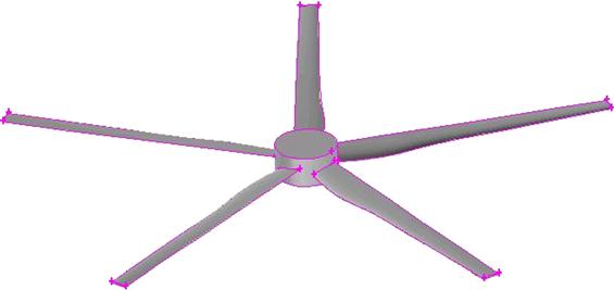
It might be a little difficult to carry out the numerical simulations on the SCPPSs coupled with the collector, chimney, and turbine. In this work, the main dimensions of the physical model shown in Table 5.1 were selected according to the Spanish prototype [1], with a 3-blade or 4-blade pressure-staged turbine with CLARK aerofoil installed at the bottom of the chimney. Tables 5.2 and 5.3 show in detail the parameters of the aerofoil type and blade section. Moreover, numerical simulation on the MW-graded SCPPS coupled with a 5-blade pressure-staged turbine with CLARK aerofoil has also been carried out, in which the physical model of the turbine is shown in Fig. 5.2. The energy storage layer is not included in the SCPPS because it is not necessary to take the energy storage layer into consideration when carrying out the steady state numerical simulation.

5.3 Mathematical Models

5.3.1 In the Collector and Chimney Regions

Some assumptions should be taken into account to simplify the problem to get the performance of the SCPPS under load condition. The whole system should be divided into three regions: the collector, the turbine, and the chimney. For the collector and chimney regions, conventional methods of numerical simulation could be used to give reasonable results, while air flow in the turbine region should be characterized by the control equations in a rotating reference frame.

For the natural convection system, it might be necessary to take into account the value of Ra Number, which can be used as a criteria for laminar and turbulent flow in the system.

$Ra=\frac{g\beta \left(T_h-T_c\right)L^3}{\alpha \nu }$ (5.1)

(5.1)

where $T_h$, $T_c$ are the highest and the lowest temperature of the system, respectively, and L is the height of the collector. It shows, by simple analysis, that the Ra Number of the SCPPS is higher than the critical Ra number, 10⁹, which means that turbulent flow happens in almost the whole system except for the entrance of the collector inlet. So the control equations including the continuity equation, momentum equation, energy equation, and the standard $k-\epsilon$ equation in the collector and chimney regions can be written as follows:

Continuity equation:

$\frac{\partial \rho }{\partial t}+\frac{\partial (\rho u)}{\partial x}+\frac{\partial (\rho v)}{\partial y}+\frac{\partial (\rho w)}{\partial z}=0$ (5.2)

(5.2)

Momentum equations:

$\frac{\partial (\rho u)}{\partial t}+\frac{\partial (\rho uu)}{\partial x}+\frac{\partial (\rho vu)}{\partial y}+\frac{\partial (\rho wu)}{\partial z}=-\frac{\partial p}{\partial x}+\mu \left(\frac{{\partial }^{2}u}{\partial x^2}+\frac{{\partial }^{2}u}{\partial y^2}+\frac{{\partial }^{2}u}{\partial z^2}\right)$ (5.3)

(5.3)

$\frac{\partial (\rho v)}{\partial t}+\frac{\partial (\rho uv)}{\partial x}+\frac{\partial (\rho vv)}{\partial y}+\frac{\partial (\rho wv)}{\partial z}=-\frac{\partial p}{\partial y}+\mu \left(\frac{{\partial }^{2}v}{\partial x^2}+\frac{{\partial }^{2}v}{\partial y^2}+\frac{{\partial }^{2}v}{\partial z^2}\right)$ (5.4)

(5.4)

$\frac{\partial (\rho w)}{\partial t}+\frac{\partial (\rho uw)}{\partial x}+\frac{\partial (\rho vw)}{\partial y}+\frac{\partial (\rho ww)}{\partial z}=\rho g\beta \left(T-T_{\infty }\right)+\mu \left(\frac{{\partial }^{2}w}{\partial x^2}+\frac{{\partial }^{2}w}{\partial y^2}+\frac{{\partial }^{2}w}{\partial z^2}\right)$ (5.5)

(5.5)

Energy equation:

$\frac{\partial \left(\rho cT\right)}{\partial t}+\frac{\partial \left(\rho cuT\right)}{\partial x}+\frac{\partial \left(\rho cvT\right)}{\partial y}+\frac{\partial \left(\rho cwT\right)}{\partial z}=\lambda \left(\frac{{\partial }^{2}T}{\partial x^2}+\frac{{\partial }^{2}T}{\partial y^2}+\frac{{\partial }^{2}T}{\partial z^2}\right)$ (5.6)

(5.6)

k and $\epsilon$ equations:

$\frac{\partial }{\partial t}\left(\rho k\right)+\frac{\partial }{\partial x_i}\left(\rho k{u}_i\right)=\frac{\partial }{\partial x_j}\left(\left(\mu +\frac{{\mu }_t}{{\sigma }_k}\right)\frac{\partial k}{\partial x_j}\right)+G_k+G_b-\rho \epsilon +S_k$ (5.7)

(5.7)

$\frac{\partial }{\partial t}\left(\rho \epsilon \right)+\frac{\partial }{\partial x_i}\left(\rho \epsilon u_i\right)=\frac{\partial }{\partial x_j}\left(\left(\mu +\frac{{\mu }_t}{{\sigma }_{\epsilon }}\right)\frac{\partial \epsilon }{\partial x_j}\right)+C_{1\epsilon }\left(G_k+C_{3\epsilon }{G}_b\right)-C_{2\epsilon }\rho \frac{{\epsilon }^2}{k}+S_{\epsilon }$ (5.8)

(5.8)

In the equations above, ${\mathit{G}}_{\mathit{k}}$ represents the generation of turbulence kinetic energy due to the mean velocity gradients, and ${\mathit{G}}_{\mathit{b}}$ is the generation of turbulence kinetic energy due to buoyancy. For the standard $k-\epsilon$ models, the constants have the following values [22]:

$C_{1\epsilon }=1.44,C_{2\epsilon }=1.92,C_{\mu }=0.09,{\sigma }_k=1.0,{\sigma }_{\epsilon }=1.3.$

5.3.2 In the Turbine Region

When successfully creating models of the collector and chimney regions using Gambit, we will typically analyze the fluid flow in an inertial reference frame, that is, in a nonaccelerating coordinate system using FLUENT. However, the air flow in the turbine region is different from that in the collector and the chimney regions, and it also rotates with the blades at a certain velocity in the radial direction besides passing through the whole region, which makes it very difficult for us to carry out the numerical simulation. Fortunately, however, FLUENT has the ability to model flows in a rotating reference frame, in which the acceleration of the coordinate system is included in the equations of motion describing the fluid flow. Such flow as in the turbine region of the SCPPSs can also be modeled in a coordinate system that is moving with the rotating equipment and thus experiences a constant acceleration in the radial direction. When the flow in the turbine region is defined in a rotating reference frame, the rotating boundaries become stationary relative to the rotating frame, because they are moving at the same speed as the reference frame. The turbine-chimney interaction could be treated by applying the multiple reference frame (MRF) model.

Thereby, when the equations of motion are solved in a rotating reference frame, the acceleration of the fluid is augmented by additional terms that appear in the momentum equations. The absolute velocity and the relative velocity are related by the following equation:

${{\displaystyle \stackrel{\rightharpoonup }{v}}}_r={\displaystyle \stackrel{\rightharpoonup }{v}}-\left({\displaystyle \stackrel{\rightharpoonup }{\mathrm{\Omega }}}\times {\displaystyle \stackrel{\rightharpoonup }{r}}\right)$ (5.9)

(5.9)

where, ${\displaystyle \stackrel{\rightharpoonup }{\mathrm{\Omega }}}$ and ${\displaystyle \stackrel{\rightharpoonup }{r}}$ are the angular velocity vector and position vector in the rotating frame, respectively. So the momentum equation for the rotation coordinate system can be obtained as follows:

$\frac{\partial }{\partial t}\left(\rho {\displaystyle \stackrel{\rightharpoonup }{v}}\right)+\nabla \cdot \left(\rho {{\displaystyle \stackrel{\rightharpoonup }{v}}}_r{\displaystyle \stackrel{\rightharpoonup }{v}}\right)+\rho \left({\displaystyle \stackrel{\rightharpoonup }{\mathrm{\Omega }}}\times {\displaystyle \stackrel{\rightharpoonup }{r}}\right)=\nabla \cdot \left(\mu \nabla {{\displaystyle \stackrel{\rightharpoonup }{v}}}_r\right)+S_{{{\displaystyle \stackrel{\rightharpoonup }{v}}}_r}$ (5.10)

(5.10)

Substituting Eq. (5.9) into Eq. (5.10) yields:

$\frac{\partial }{\partial t}\left(\rho {{\displaystyle \stackrel{\rightharpoonup }{v}}}_r\right)+\nabla \cdot \left(\rho {{\displaystyle \stackrel{\rightharpoonup }{v}}}_r{\stackrel{\rightharpoonup }{v}}_r\right)+\rho \left(2{\displaystyle \stackrel{\rightharpoonup }{\mathrm{\Omega }}}\times {\displaystyle \stackrel{\rightharpoonup }{r}}+{\displaystyle \stackrel{\rightharpoonup }{\mathrm{\Omega }}}\times {\displaystyle \stackrel{\rightharpoonup }{\mathrm{\Omega }}}\times {\displaystyle \stackrel{\rightharpoonup }{r}}\right)+\rho \frac{\partial {\displaystyle \stackrel{\rightharpoonup }{\mathrm{\Omega }}}}{\partial t}\times {\displaystyle \stackrel{\rightharpoonup }{r}}=\nabla \cdot \left(\mu \nabla {{\displaystyle \stackrel{\rightharpoonup }{v}}}_r\right)+S_{{{\displaystyle \stackrel{\rightharpoonup }{v}}}_r}$ (5.11)

(5.11)

where $\rho \left(2{\displaystyle \stackrel{\rightharpoonup }{\mathrm{\Omega }}}\times {\displaystyle \stackrel{\rightharpoonup }{r}}+{\displaystyle \stackrel{\rightharpoonup }{\mathrm{\Omega }}}\times {\displaystyle \stackrel{\rightharpoonup }{\mathrm{\Omega }}}\times {\displaystyle \stackrel{\rightharpoonup }{r}}\right)$ is the Coriolis force.

For flows in rotating zones, the continuity equation can be written as follows:

$\frac{\partial \rho }{\partial t}+\nabla \cdot \left(\rho \cdot {\overrightarrow{v}}_r\right)=0$ (5.12)

(5.12)

The maximal available energy of the updraft air in the system could be derived as follows:

$N=V\mathrm{\Delta }p$ (5.13)

(5.13)

where, V and $\mathrm{\Delta }p$ are the mass flow rate and the pressure drop across the turbine, respectively. The power output, or the technical work, from the turbine can be obtained:

$P_t=\frac{2\pi nI}{60}$ (5.14)

(5.14)

where, n and I are the rotation speed and the total blade moments of the turbine, respectively. From Eqs. (5.13) and (5.14), the turbine efficiency can be obtained:

$\eta =\frac{P_t}{N}=\frac{2\pi nI}{60V\mathrm{\Delta }p}$ (5.15)

(5.15)

5.4 Near-Wall Treatments for Turbulent Flows

Turbulent flows are significantly affected by the presence of walls. The near-wall modeling significantly impacts the fidelity of numerical solutions, inasmuch as walls are the main source of mean vorticity and turbulence. In the near-wall zone the solution variables have large gradients, and the momentum and other scalar transports occur most vigorously. Therefore, accurate representation of the flow in the near-wall zone determines successful predictions of wall-bounded turbulent flows.

The wall function approach, which uses semiempirical formulas to bridge the viscosity-affected zone between the wall and the fully-turbulent zone, will be adopted in this model because it can substantially save computational resources, obviate the need to modify the turbulence models to account for the presence of the wall, and because the viscosity-affected near-wall zone, in which the solution variables change most rapidly, does not need to be resolved. In addition, this approach is economical, robust, and reasonably accurate. It is a practical option for the near-wall treatments for industrial flow simulations.

Based on the proposal of Launder and Spalding [23], the law-of-the-wall for mean velocity yields:

$U^{*}=\frac{1}{\kappa }\ln \left(E{Y}^{*}\right)$ (5.16)

(5.16)

where

$U^{*}\equiv \frac{U_P{C}_{\mu }^{1/4}{k}_P^{1/2}}{{\tau }_w/\rho }$ (5.17)

(5.17)

$Y^{*}\equiv \frac{\rho C_{\mu }^{1/4}{k}_p^{1/2}{Y}_p}{\mu }$ (5.18)

(5.18)

and U_P, K_P, Y_P are the mean velocity, turbulence kinetic energy of the fluid at point P and distance from point P to the wall, respectively. U*is the nondimensional velocity and Y* is the nondimensional distance from the computational point to the wall.

The logarithmic law for mean velocity is employed when Y*>11.225. When the mesh is such that Y*<11.225 at the wall-adjacent cells, the laminar stress-strain relationship can be written as U*=Y*. Reynolds’ analogy between momentum and energy transport gives a similar logarithmic law for mean temperature. As in the law-of-the-wall for mean velocity, the law-of-the-wall for temperature employed comprises two different laws: linear law for the thermal conduction sublayer where conduction is important and logarithmic law for the turbulent zone where effects of turbulence dominate conduction shown as follows:

$T*=\mathrm{Pr}Y*+\frac{1}{2}\rho \mathrm{Pr}\frac{C_{\mu }^{1/4}{k}_P^{1/2}}{\dot{q}}{U}_P^2\left(Y*<Y_T^{*}\right)$ (5.19)

(5.19)

$\begin{array}{l}T*={\mathrm{Pr}}_t\left(U*+B\right)+\frac{1}{2}\rho \frac{C_{\mu }^{1/4}{k}_P^{1/2}}{\dot{q}}\left({\mathrm{Pr}}_t{U}_p^2+\left(\mathrm{Pr}-{\mathrm{Pr}}_t{U}_c^2\right)\right)\left(Y*<Y_T^{*}\right)\hfill \end{array}$ (5.20)

(5.20)

Where B is computed by using the formula given by Jayatilleke [24]:

$\mathit{B}=9.24\left({\left(\frac{\mathit{\sigma }}{{\mathit{\sigma }}_{\mathit{t}}}\right)}^{3/4}-1\right)\left(1+0.28e^{-0.007\mathit{\sigma }/{\mathit{\sigma }}_{\mathit{t}}}\right)$ (5.21)

(5.21)

and T_P, T_W are temperature at the cell adjacent to wall and temperature at the wall, respectively, U_C is mean velocity magnitude at Y*=Y*_T.

The nondimensional thermal sublayer thickness, ${\mathit{Y}}_{\mathit{T}}^{*}$, in Eqs. (5.19) and (5.20) is computed as the Y* value at which the linear law and the logarithmic law intersect, given the Pr value of the water being modeled.

5.5 Numerical Simulation Method

The collector inlet condition is variable under different solar radiation as the free convection happens in the whole system. Thereby, some important parameters such as the collector inlet velocity, mass flow rate of the system, pressure drop across the turbine, and the correlation between the solar radiation and the rotational speed of the turbine are unknown for the numerical simulation of the system including the collector, turbine, and chimney regions. Fortunately, however, different rotational speed of the turbine could be given in advance without taking into account the variation of the solar radiation intensity, which implies that not much more attention need be paid to the correlation between the solar radiation and the rotational speed of the turbine.

It is necessary to point out that the rotational direction of the turbine in the solar chimney might have significant effect on the validity of the results of numerical simulation. If the fluid impels the turbine to rotate, which transforms the energy of the air with relative higher temperature and velocity into technical work, the mass flow rate of the system and chimney outlet velocity will decrease compared with those on no load condition. While the turbine blades will impel the air flows out of the chimney, if the rotational speed of the turbine is set in an opposite direction, therefore, the mass flow rate of the system and the chimney outlet velocity will increase inversely.

Numerical simulations of the SCPPSs should be based on some assumptions shown as follows: (1) Constant environment conditions, including uniform solar radiation (800 W/m²), ambient temperature, and inlet air temperature, should be taken into account. (2) Axisymmetric air flow in the collector inlet, that is, nonuniform heating of the collector surface in terms of the sun’s altitude angle is neglected. (3) Heat loss through the wall of the chimney is neglected. (4) The Boussinesq approximation is assumed to be valid for the variation of air density in the whole system.

The main boundary conditions, derived by energy equilibrium equations, are shown in Table 5.4 for mass, momentum, and energy conservation equations, and the temperature profiles of the ground and the canopy in the collector could be different parabolic functions of the collector radius by taking into account the axisymmetric air flow in the collector shown in the second assumption above, and the functions will vary with different solar radiations.

Table 5.4

Boundary Conditions and Model Parameters

Place	Type	Value
Surface of the ground	Wall	$T=f_1(r)\mathrm{K}$
Surface of the canopy	Wall	$T=f_2(r)\mathrm{K}$
Surface of the chimney	Wall	qchim=0 W/m2
Inlet of the collector	Pressure inlet	pr,i=0 Pa, T0=293K
Outlet of the chimney	Pressure outlet	pr,o=0 Pa
Turbine rotational speed		$\omega =n$ rpm

As mentioned above, both stationary and moving regions are selected for the numerical simulation on the SCPPS coupled with the turbine. Three different models, that is, the MRF model, the mixing plane model, and the sliding mesh model, could be used to solve the problem involved in FLUENT, of which the MRF model is the simplest. It is a steady-state approximation in which individual cell zones move at different rotational speeds. Interior faces could be selected for the boundaries (ie, the collector and the turbine regions, the turbine and the chimney regions) between reference frames. In addition, simulation results independent of the meshes should be taken into consideration.

5.6 Results and Discussions

5.6.1 Validity of the Method for the Spanish Prototype

To validate the simulation method used by the author in this chapter, numerical simulation results are compared with the experimental result [2] for the Spanish prototype with a 4-blade turbine which is set up at the bottom of the chimney.

When the solar radiation is 800 W/m², 35 kW technical work could be extracted from the Spanish prototype with a 4-blade turbine [2]. Fig. 5.3 shows the simulation results of the SCPPS with a 4-blade designed in this chapter and Fig. 5.4 shows the velocity vectors in detail in the turbine region. It can be easily seen from Fig. 5.3 that the experimental result is in the scope of the simulation results, and the maximum power output from the simulation results is a little higher than the experimental result, and that the rotational speed of the turbine is 80 rpm, 25% less than that of the experimental result [2]. In addition, as velocity changes greatly around the turbine blades, especially at the tip of the blade, air velocity might be a few times larger than the main flow in the chimney.

5.6.2 Characteristic of 3-Blade Turbine for the Spanish Prototype

Fig. 5.5 shows the effect of different turbine rotational speeds on the average temperature and velocity of the chimney outlet. From the figure, we can see that the average velocity of the chimney outlet decreases significantly and the average temperature inversely with the increase of the turbine rotational speed. The reason is that, when all the other parameters such as the environment parameters and the solar radiation are constant, large resistant force caused by the blades of the turbine occurs with the increase of the turbine rotational speed. And with the increase of the resistant force, the mass flow rate of the system might decrease and then the air velocity of the chimney outlet would decrease accordingly. In addition, the decrease of the air velocity might result in a longer time for the air inside the collector to absorb energy from the surface of the energy storage layer while passing through the collector. Thereby, the average temperature of the chimney outlet increases prominently.

Fig. 5.6 shows the effect of the turbine rotational speed on the pressure drop across the turbine and the mass flow rate of the Spanish prototype. When the turbine rotational speed is lower than 50 rpm, the mass flow rate is higher than 1000 kg/s. The mass flow rate decreases almost linearly with the increase of the turbine rotation speed, which indicates that the resistant force changes significantly with the increase of the turbine rotational speed. It can be predicted that the mass flow rate might decrease more notably when the blades number of the turbine increases.

Besides, we can see from Fig. 5.6 that the pressure drop across the turbine increases remarkably with the increase of the turbine rotation speed. The increase of pressure drop across the turbine means that an increasing part of the driving force of the SCPPSs is used to drive the turbine. The variation trend of pressure drop with the turbine rotation speed decreases when the turbine rotation speed surpasses 200 rpm, which means that the utilization of pressure drop of the system reaches its limitation and it is not necessary to increase the turbine rotation speed any more.

Fig. 5.7 shows the relationship between the turbine rotational speed and the maximum available energy, power output, and turbine efficiency. For the kW-graded turbine model designed in this work, the maximum available energy is a little above 100 kW when the turbine rotational speed reaches 180 rpm, while the power output and turbine efficiency reach their peak values when the rotational speed reaches 210 rpm. The maximum power output is about 50 kW, which is identical to the designed data of the Spanish prototype, and the turbine efficiency is near 50%, which could reach a much higher value with some optimization for the turbine.

Compared with the Spanish prototype turbine designed with 4 blades, the turbine rotational speed of the 3-blade turbine in this work is much larger, the reasons are as follows: firstly, the number of turbine blades is a significant factor to the rotational speed which will notably increase once the blade number decreases with the same power output, and simulation results show that power output of 50 kW could not be extracted from the solar chimney power plant prototype if a 2-blade turbine is selected to be installed at the bottom of the chimney. Secondly, the turbine blades are a little longer and slimmer to some extent, and we will get higher turbine efficiency and larger power output with the optimization of the turbine blade. Although the 3-blade turbine model is different from the Spanish prototype with 4 blades, there is no doubt that the turbine rotational speed will decrease remarkably when the number of blades of the turbine increases compared with the results shown in Fig. 5.3.

The numerical simulation results shown in Figs. 5.5–5.7, although a little different from the experimental data [2], keep to the principles of heat transfer and flow of free convection system and the operation theory of pressure-staged turbine. Therefore, the numerical simulation method advanced in this chapter is feasible, and the results might be more easily accepted than the 2-D simulation results [14]. In addition, it is a good way to predict the power output of large-scale solar chimney power plant with one or several turbines. The following section shows the results of the MW-graded SCPPSs including a turbine with 5 blades.

5.6.3 Results for MW-Graded Solar Chimney

In order to provide a reference for the commercial SCPPSs, numerical simulations have also been carried out for the MW-graded solar chimneys in this section. A physical model of the 5-blade turbine is shown in Fig. 5.2 and the detailed parameters of the CLARK aerofoil are the same as for the kW-graded prototype turbine shown in Tables 5.2 and 5.3. Other dimensions of the MW-graded solar chimney are shown in Table 5.1.

Fig. 5.8 shows the effect of the turbine rotational speed on the average velocity and temperature of the chimney outlet. Similarly, the average velocity of the chimney outlet decreases but the temperature increases with the increase of the rotational speed of the turbine. The main difference between the MW-graded model and the kW-graded model lies in that, with the increase of the rotational speed of the turbine, velocity decreases significantly, while temperature increases slightly. The reasons are as follows: pressure drop across the turbine results in a significant effect on the mass flow rate of the system, and the increase of pressure drop across the turbine can cause a remarkable decrease of the fluid velocity, while the temperature of the chimney outlet changes slightly only because the collector radius is large enough for the air to have enough time to absorb heat energy inside.

Fig. 5.9 shows the effect of the turbine rotational speed on the pressure drop and the mass flow rate across the turbine. As can been seen from this figure, when the turbine rotational speed is lower than 50 rpm, pressure drop across the turbine increases rapidly, while the mass flow rate decreases notably. Inversely, when the rotational speed exceeds 50 rpm, changes of the pressure drop and mass flow rate could be neglected. So it can be estimated, according to the results, that the operation rotational speed of the turbine might be selected as 50 rpm because the power output and turbine efficiency may significantly change with the turbine pressure drop and system mass flow rate across the turbine.

Fig. 5.10 shows the effect of the turbine rotational speed on the maximum available energy, power output, and turbine efficiency of the MW graded system. It can be easily seen that when the turbine rotational speed is 50 rpm, the maximum available energy reaches the peak value exactly; but the power output and efficiency could not reach their maximum values. When the turbine rotational speed is 40 rpm, the maximum power output surpasses 10 MW, and the maximum turbine efficiency also reaches its peak value, and then the power output and turbine efficiency decrease significantly with the increase of the turbine rotational speed, which means that the best operation rotational speed is 40 rpm for the 5-blade turbine.

Apparently, the 5-blade turbine model designed by the author for MW-grade SCPPS might be unsuitable to be put into practice, as it is difficult to design a single turbine with the output of 10 MW in the present technical conditions. In addition, the aerofoil and detail parameters of the turbine blades need to be further optimized to get much higher power output and turbine efficiency. But there might be a right way in the near future to make a design of several turbines with the rated power output about 6 MW for a large-scale SCPPS.

5.7 Conclusions

A numerical simulation method for the SCPPS including the turbine is presented in this chapter. The results for the Spanish prototype with a 3-blade turbine show that, with the increase of the turbine rotational speed, the average velocity of the chimney outlet and the system mass flow rate decrease, the average temperature of the chimney outlet and the turbine pressure drop inversely, so the maximum available energy, power output, and efficiency of the turbine each have a peak value.

The numerical simulation for the MW-grade SCPPS has been carried out to give a reference for the design of large-scale SCPPSs. For a solar chimney with a chimney 400 m in height and 30 m in radius, a collector 1500 m in radius, and a 5-blade turbine designed in this chapter, the maximum power output and turbine efficiency is about 10 MW and 50%, respectively.