
7
Remote Sensing of the Earthquake Deformation Cycle
Mathilde MARCHANDON1, Tim J.WRIGHT2 and James HOLLINGSWORTH1
1ISTerre, Grenoble, France
2COMET, University of Leeds, UK
7.1. Introduction
Our most basic understanding of the earthquake deformation cycle comes from the theory of the elastic rebound elaborated by Reid (1910) after the 1906 San Francisco earthquake. As tectonic plates slowly move, elastic strain is accumulated on faults. When the accumulated strain is large enough to overcome the fault strength, all the strain is suddenly released by a sudden slip on the fault, producing an earthquake. Fault slip induces displacements at the ground surface that can be measured and used to better understand earthquake processes. Displacements can also be measured during the long “inter-seismic” buildup to earthquakes and the rapid “post-seismic” transients that follow many earthquakes.
Before the advent of space-based geodesy, surface displacement measurements could only be made at sparse locations and only in regions where a surveyed network was in place before the earthquake. Thirty years ago, the development of the interferometric synthetic aperture radar (InSAR) technique revolutionized our ability to measure the surface displacement fields of earthquakes. By comparing the phase of RADAR satellite images, InSAR can precisely measure the surface displacements of earthquakes with nearly complete spatial continuity. Since its first application for measuring the coseismic displacements of the 1992 Landers earthquake (Massonnet et al. 1993), and thanks to the dramatic increase in data availability, InSAR has been applied to document the surface deformation of more than 100 earthquakes (Funning and Garcia 2019). InSAR also allows us to track the deformation produced by inter-seismic loading and aseismic transient processes, such as post-seismic deformation or inter-seismic creep events (e.g. Peltzer et al. 1998; Wright et al. 2001b; Rousset et al. 2016). InSAR data have been critical in enabling scientists to constrain the distribution of slip and fault geometry at depth, determine the rheology of the lithosphere and assess the frictional properties of fault zones. Furthermore, InSAR data can now be used to map inter-seismic loading over thousands of square kilometers, maps that might be used in the near future to improve models of seismic hazard assessment (Weiss et al. 2020).
More recently, another space-based geodetic technique, optical correlation, has been developed. This technique makes it possible to measure the horizontal displacements of an earthquake by measuring the pixel shifts between two pictures of the ground. The vertical component of the displacement can also be assessed if stereoscopic images are available. Although less precise than InSAR, this technique has the considerable advantage of being able to measure the near-field deformation of surface-rupturing earthquakes, where InSAR often cannot provide measurements due to the decorrelation of the interferometric phase. The geometry of the surface rupture and the surface slip can be readily observed at spatial resolutions not achievable by field investigations (or other geodetic techniques). This new type of data has allowed researchers to better characterize the surface rupture of large continental earthquakes (e.g. Michel and Avouac 2002), estimate the amount of deformation occurring in the volume around the fault (e.g. Zinke et al. 2014) and better constrain fault slip models (e.g. Xu et al. 2016).
In this chapter, we review the main advances brought by InSAR and optical correlation for our understanding of earthquake and fault mechanics. The chapter is divided into two parts. The first part provides an overview of what we have learned from 30 years of tectonic InSAR (section 7.2). Section 7.2.1 focuses on the coseismic phase of the seismic cycle, section 7.2.2 on the inter-seismic phase and section 7.2.3 on the post-seismic phase. Each section reviews the history of InSAR studies and what we have learned about faults and earthquakes from them. For a detailed review of the technical aspects of InSAR, we refer the reader to Chapters 4, 5 and 6 of this book. In the second part of the chapter, we focus on the study of surface-rupturing earthquakes using optical correlation (section 7.3). First, the advantages of the technique compared to more traditional methods are reviewed and a brief history of the technique is presented (section 7.3.1). Then, we briefly describe the general workflow used to obtain the 2D and 3D displacement field of an earthquake from optical images, as well as the main sources of error and limitations (section 7.3.2). For the theoretical aspect of optical correlation, we refer the reader to Chapter 2 of this book. In section 7.3.3, we show examples of surface displacement fields from recent and pre-modern geodesy (<1990s) for earthquakes measured by optical correlation. Finally, we review the insights on earthquake and fault mechanics brought by high-resolution optical correlation displacement fields (section 7.3.4).
7.2. What have we learned about faults from nearly three decades of tectonic InSAR?
Zebker and Goldstein (1986) were the first to demonstrate that an interferogram could be formed from two radar images. In this case, they were acquired simultaneously from an airborne platform, and the interference patterns were due to topography. Two years later, Goldstein et al. (1988) published an interferogram from two images acquired three days apart by the short-lived SeaSat mission (Barrick and Swift 1980). Shortly afterwards, Gabriel et al. (1989) proposed that differential synthetic aperture radar interferometry could be used to map small ground movements over large areas. However, it was not until the launch of the first European Remote Sensing Satellite (ERS-1) by the European Space Agency (ESA) in 1991 that there was a platform stable enough to perform differential InSAR reliably. The first coseismic interferogram by Massonnet et al. (1993), famously gracing the cover of Nature, showed the line-of-sight displacement field for the 1992 Mw 7.3 Landers earthquake in spectacular detail.
The Landers earthquake paper marked the beginning of nearly three decades of tectonic applications of InSAR, which we review below. We organize the review according to the phase of the earthquake cycle. For each phase, we describe the history of InSAR studies, how those studies have evolved and progressed over the last 30 years and what we have learned about faults from the research. The review is not intended to be an comprehensive overview of every tectonic study, and the selection of research highlighted below is certainly biased by the authors’ own experiences and prejudices. We were motivated by being challenged with the question, “what have we learned from InSAR about tectonics and faulting?”, and we apologize if what follows reads like an answer to Monty Python’s famous question, “What have the Romans ever done for us?”1 (Jones 1979).
7.2.1. Coseismic deformation
7.2.1.1. History and recent progress in coseismic InSAR studies
Before InSAR, it was extremely challenging to measure surface displacements caused by earthquakes. Earthquakes in a specific location are rare, so taking displacement measurements relied on serendipity – earthquakes could only be measured if precise survey data had been acquired prior to the event (e.g. Stein and Barrientos 1985) or if natural data, such as uplifted shorelines, could be interpreted (e.g. Plafker 1965). As such, displacements from around 20 earthquakes or fewer had been measured (Wright 2000). Data from these studies appeared to confirm the elastic rebound theory popularized by Reid (1910) but were in general too sparse to be used to determine details of earthquake mechanisms and slip distributions.
The widespread availability of SAR data acquired before and after earthquakes, along with the proliferation of measurements from global navigation satellite systems (such as the US Global Positioning System), means that spatially dense, precise observations of surface displacements are now available for almost all recent earthquakes where there is significant (1 cm or more) movement of the land surface. Earthquake deformation has been mapped for events ranging in size from small (Mw ∼ 5), shallow (< 10 km) events on continental faults (e.g. Lohman and Simons 2005) to on-land deformation from great earthquakes on subduction megathrusts (e.g. Kobayashi et al. 2011).
The ability of InSAR to capture coseismic deformation relies on pre- and post-event data existing. Mission managers at the ESA recognized this opportunity and implemented systematic background acquisition plans for the ERS and Envisat missions (Attema et al. 2000; Miranda et al. 2013) that ensured data were acquired regularly over tectonically active areas, although the 35-day revisit time and relatively wide orbital tube for ERS and Envisat meant that the method did not work for many earthquakes. Nevertheless, by the end of the Envisat mission in 2010, studies on 60 earthquakes using InSAR data had been published (Weston et al. 2012).
The launches of the EU Copernicus Sentinel-1 C-band SAR satellites, Sentinel-1A (launched in 2014) and Sentinel-1B (launched in 2016), have radically increased the volume and quality of SAR data available for InSAR analysis. Together, the satellite constellation can acquire SAR data with a six-day revisit, and a small orbital tube means that interferograms can be formed between all acquisitions (Torres et al. 2012). Funning and Garcia (2019) examined Sentinel-1A data for 35 “potentially detectable” earthquakes that occurred between April 2015 and December 2016, finding that around 70% of these had coherent signals. However, they found that 31% of the events, mostly in vegetated low latitude regions, could not be detected with the available C-band data from Sentinel-1A. Since that study, Sentinel-1 has increased its duty cycle and acquires data globally every 6 or 12 days, depending on the location, including on both ascending and descending tracks in the tectonic belts. Several automatic systems have been built that provide rapid response interferometric data to the community for analysis (e.g. Barnhart et al. 2019; Lazeck`y et al. 2020).
C-band data (∼6 cm wavelength) can suffer from poor coherence in vegetated areas. Further improvements can be made in these cases using data from longer-wavelength L-band SAR missions (∼20 cm wavelength), such as from PALSAR on the Japanese ALOS-2 satellite (Rosenqvist et al. 2014). The launch of the joint US–India L-band SAR mission NISAR, currently scheduled for 2022 (Rosen et al. 2017), will ensure L-band SAR data are acquired globally for all ascending and descending passes with a 12-day revisit time. The EU Copernicus program is also planning an operational L-band SAR mission to complement the C-band data from Sentinel-1 (Elliott 2020).
7.2.1.2. What have we learned about faults from InSAR studies of coseismic deformation
For individual earthquakes on land, the detailed maps of surface deformation provided by InSAR typically provide more accurate locations and depths than are available from global teleseismic seismology, often revealing significant mislocations in the seismic catalogues (Weston et al. 2011). For shallow events larger than Mw ∼ 6, it is usually possible to derive detailed slip distributions from InSAR, again with the geodetic solutions resolving finer spatial details than is possible from global seismology. The large number of dense geodetic earthquake deformation observations has led to a significant increase in our knowledge of earthquake behavior in several key areas. Here, we summarize some of the major advances in our understanding about faults and earthquakes that have been made possible through InSAR observations.
Fault complexity: a key area where our understanding of earthquakes has changed because of the availability of precise, dense geodetic data from InSAR is earthquake complexity. Earthquakes with Mw less than around 6 can typically be modeled with uniform slip on a single rectangular fault plane in an elastic half-space (Okada 1985), particularly if they do not rupture the surface. However, larger, shallow earthquakes usually require more complex models of variable slip on segmented faults or multiple fault strands (e.g. Elliott et al. 2016). Several recent earthquakes, including the 2010 Mw7.1 Darfield (New Zealand) earthquake (Elliott et al. 2012), the 2010 Mw7.2 El Mayor Cucapeh (Mexico) earthquake (Huang et al. 2017) and the 2019 Mw6.4/7.1 Ridgecrest (USA) sequence (Xu et al. 2020), have required significant complexity to match the geodetic observations, with slip occurring on multiple fault strands.
The type example of a complex, multi-fault rupture is the 2016 Mw7.8 Kaikoura (New Zealand) earthquake, which ruptured more than 170 km of faults in the northeast part of the South Island of New Zealand (Figure 7.1; Hamling et al. 2017). In total, more than 20 crustal faults had surface ruptures, and these include faults that were previously mapped as well as previously unknown structures (Litchfield et al. 2018). Both crustal faults and the deeper subduction interface may have failed simultaneously (Furlong and Herman 2017). The earthquake defied conventional wisdom about the ability of fault segmentation to arrest/control rupture; the rupture appeared to jump across fault stepovers as high as 15–20 km (Hamling et al. 2017). Without the detailed geodetic imaging work from InSAR and optical correlation, it would have been extremely challenging for field teams to map the complexity of this earthquake – scarps from surface ruptures erode very rapidly in New Zealand. The new understanding of the potential for complex, multi-fault ruptures is now being incorporated in the latest generation of seismic hazard models.
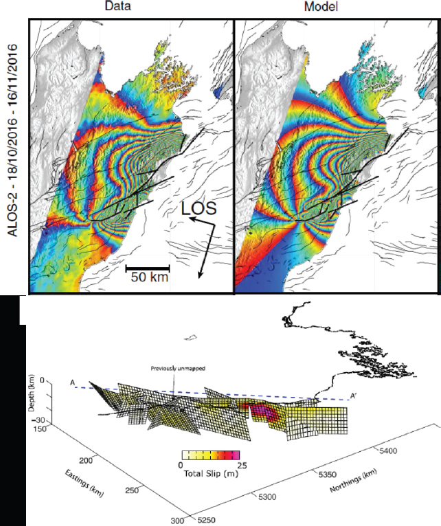
Figure 7.1. Deformation and model for the 2016 Kaikoura earthquake, adapted from (Hamling et al . 2017). Top left: coseismic interferogram from ALOS-2. Top right: predicted interferogram using dislocation models. Bottom: 3D view of the complex slip model for the earthquake, showing only the crustal faults that were modeled as slipping in the event. For a color version of this figure, see www.iste.co.uk/cavalie/images.zip
Surface versus deep fault slip during earthquakes: another area where dense geodetic imaging data have changed our understanding of earthquakes is the relationship between fault slip seen at the surface in an earthquake and the slip that occurs at depth. Earthquakes on “blind” thrust faults, where minimal slip reaches the surface, were known before InSAR (e.g. Yielding et al. 1981; Ekström et al. 1992), but we now know that for all types of earthquake, the surface slip is in fact only a partial guide to the slip that occurs at depth. For example, modeling of the 1995 Mw6.4 Dinar earthquake, a normal-faulting earthquake in southwest Turkey, requires 1.2–1.4 m of slip as shallow as 2 km beneath the surface, but the maximum observed surface rupture magnitude was only 0.25 m (Fukahata and Wright 2008). Similarly, in the 2003 Mw6.5 Bam earthquake (strike-slip, Iran), models require 2–3 m of slip at ∼ 4 km depth, but the maximum surface slip was again 0.25 cm. This observation is not limited to moderate earthquakes – Kaneko and Fialko (2011) compared the slip profiles of the Bam earthquake and four other strike-slip faults with Mw > 7.1, showing that they all had a shallow slip deficit as high as 60%. Although more detailed analysis of near-field date by Xu et al. (2016) reduced the magnitude of the discrepancy for some of these earthquakes, it is clear that the surface slip often only provides a minimum estimate for the fault slip that occurred in the subsurface.
The observation of a discrepancy between surface observations and slip at depth has important implications for studies of paleoseismology – magnitudes estimated from paleo-offset data and empirical relationships between slip and magnitude (Wells and Coppersmith 1994) are likely to be lower bounds of the true magnitude of earthquakes. The causes and implications of the shallow slip deficit (SSD) have also been investigated. There are several plausible explanations. The first is that fault slip branches near the surface onto multiple strands, and without precise and detailed near-field data, this can map into an apparent deficit (e.g. Xu et al. 2016). A second possibility is that friction in the shallowest portion of the fault is velocity-strengthening – some shallow slip then occurs as afterslip or inter-seismic creep. Hussain et al. (2016) investigated this possibility for part of the North Anatolian Fault that ruptured in the 1999 Izmit/Kocaeli earthquake, finding that without additional periods of rapid shallow slip, this mechanism could only partially explain the observed shallow slip deficit. Finally, it is possible that inelastic distributed deformation, for example due to folding, accommodates some of the strain in the shallowest portion of the fault. It seems likely that these mechanisms may operate concurrently in some cases. High-resolution near-field displacement data from optical image correlation is invaluable for investigating these mechanisms (see discussion later in this chapter).
Dynamic triggering: although geodetic imaging techniques like InSAR provide a snapshot of the total deformation that occurs between two image acquisitions, the dense spatial coverage of the observations has revealed unexpected deformation patterns in a few instances that were initially missed by seismology. One of the best observations of dynamic triggering is from Pagli et al. (2003), who observed deformation on the Reykjanes Peninsula in Iceland that was consistent with an undetected Mw5.8 strike-slip earthquake. They showed that the earthquake was dynamically triggered by a Mw6.6 earthquake around 100 km away. The triggered earthquake was not initially detected by seismic networks because the seismic waveform was partially hidden by the waveforms from the larger event.

Figure 7.2. Surface displacements in the 1995Mw 6.4 Dinar (Turkey) earthquake. Left: Coseismic interferogram formed between an ERS-1 acquisition on August 13, 1995 and an ERS-2 acquisition on January 1, 1996, unwrapped and rewrapped with 10 cm fringes, draped on Shuttle Radar Topography Mission (SRTM) topography. The red line shows the surface rupture location. Right: Profiles along the white line in the map showing topography and range change (negative values are movement away from the satellite in this figure), and a cross-section showing fault geometry and seismicity within two weeks of the mainshock (from the Kandilli Observatory catalogue; foreshocks: open circles, aftershocks: filled, mainshock: star). The red line is the observed ground movement from InSAR and the black dashed line is a model with uniform slip. Elastic dislocation models require 1.2–1.4 m of slip at depth; however, the largest observed surface rupture in the field was 0.25 m (Wright et al. 1999; Fukahata and Wright 2008). For a color version of this figure, see www.iste.co.uk/cavalie/images.zip
Another beautiful example of dynamic triggering was presented by Nissen et al. (2016), who investigated an Mw7.1 reverse-faulting earthquake that occurred in Pakistan in 1997. They found that the earthquake was in fact not a single event but a doublet, with two clear areas of uplift associated with separate faults. Joint analysis of the InSAR with seismology showed that the initial rupture was followed just 19 s later by rupture of a second reverse fault, located ∼ 50 km away. Again they invoke dynamic triggering to explain the occurrence of this doublet. Dynamic triggering is also likely to have played a part in the Kaikoura (New Zealand) earthquake (Figure 7.1) discussed earlier. The potential for dynamic triggering is an additional factor that needs to be accounted for in future seismic hazard models and scenarios.
Structural control of earthquake rupture: although some earthquakes, such as Kaikoura, appear to propagate through structural barriers (Hamling et al. 2017), InSAR has documented other examples where pre-existing structure does appear to play an important role in controlling earthquake rupture. Several good examples of this have been observed in the India–Asia collision zone. The 2001 Mw7.8 Kokoxili earthquake ruptured more than 400 km of the Kunlun Fault in northern Tibet, with slip reaching as high as 8 m in places. Lasserre et al. 2005 showed that areas of significant moment release corresponded to the first-order along-strike structural segmentation of the fault, with very low slip observed and modeled on some segment boundaries. Elliott et al. (2011) showed that depth segmentation can also act as a barrier to rupture – they investigated two Mw6.3 reverse-faulting earthquakes that occurred in the North Qaidam Thrust system (Tibet) at almost the same location but separated in time by nearly 300 days. They showed that the first of the two earthquakes ruptured the lower part of the seismogenic crust, with the later event rupturing a near continuation of the same fault plane in the upper seismogenic crust. They speculated that the gap between the two earthquakes was due to a structural barrier caused by the intersection of a reverse fault dipping in the opposite direction.
Structural control also appears to have played an important role in the 2015 Mw7.8 Gorkha (Nepal) earthquake, which partially ruptured the locked shallow Himalayan megathrust (Grandin et al. 2015; Elliott et al. 2016a). Qiu et al. (2016) used a structural geology model to show that the coseismic slip was confined to a flat region of the megathrust surrounded by two steeper ramps. They also ran dynamic simulations that showed that their fault geometry was sufficient to confine some (but not all) ruptures to the lower or upper part of the seismogenic fault; some earthquakes in their simulations were larger and ruptured the entire locked megathrust. Importantly for Nepal, the shallow, locked portion of the megathrust remains locked and has not moved following the earthquake (Ingleby et al. 2020) – the hazard remains very high there.
7.2.2. Inter-seismic deformation
7.2.2.1. History and recent progress in inter-seismic InSAR studies
Mapping inter-seismic strain accumulation with geodetic methods has been a long-standing goal of the geodetic community as it has the potential to strongly inform seismic hazard models. If Reid’s 1910 elastic rebound hypothesis is correct then measuring where strain is accumulating, and at what rate, should allow us to quantify the long-term rates of fault movement, and hence, the rate of seismicity. Elliott et al. (2016) showed that in the western US and in eastern Turkey, areas with dense GNSS coverage and high tectonic strain rates, there is a good correlation between seismicity rate and geodetic strain rate, and data from the GNSS-derived Global Strain Rate Model (Kreemer et al. 2014) have been used to make global seismicity forecasts that compare well with forecasts based on instrumental seismicity (Bird and Kreemer 2015). However, dense GNSS data are not available globally. Here, we review progress in using InSAR to measure inter-seismic strain and show that it has the potential to significantly improve strain rate models built from GNSS data alone.
Using InSAR to measure inter-seismic strain is challenging compared to using InSAR for earthquakes – the inter-seismic signal in any one short-interval interferogram is much smaller than the noise, particularly the noise arising from spatial and temporal variations in tropospheric delays. The first studies to clearly show the signature of inter-seismic strain in InSAR results were able to reduce the noise in individual interferograms by stacking a relatively small number of datasets from ERS-1 and ERS-2 with multi-year time spans (Peltzer et al. 2001; Wright et al. 2001b). With the ESA operating Envisat with a more systematic background acquisition strategy in tectonic areas, alongside increasing volumes of data from systems such as ALOS, increasing computer power, and improved algorithms (e.g. Doin et al. 2011; Agram et al. 2013; Morishita et al. 2020), an increasing number of studies have been able to map inter-seismic tectonic deformation over ever larger and/or more challenging areas (e.g. Grandin et al. 2012; Wang and Wright 2012; Tong et al. 2013; Cakir et al. 2014; Pagli et al. 2014; Hussain et al. 2018; Wang et al. 2019).
The launch of the Sentinel-1 constellation has again provided a radical increase in the volume of SAR data acquired over tectonic areas (Elliott et al. 2015). The shorter revisit time increases coherence and means that average crustal velocities can be obtained with improved accuracy. Several groups have developed tools capable of mass processing Sentinel-1 data (e.g. Bekaert et al. 2019; Foumelis et al. 2019; Lazeck`y et al. 2020), with the ESA’s Geophysical Exploitation Platform (Foumelis et al. 2019) and COMET’s LiCSAR system (Lazeck`y et al. 2020) focused on mass producing interferometric products for the continental seismic belts. Weiss et al. (2020) presented the largest regional analysis of Sentinel-1 to date, processing Sentinel-1 data using LiCSAR and LiCSBAS (Morishita et al. 2020) over 800,000 km2 of Anatolia. They produced average velocities for both ascending and descending tracks and used these in combination with GNSS data to provide east–west and vertical velocities and to estimate strain (Figure 7.3). The results reveal both large-scale features, such as the North Anatolian Fault, as well as localized deformation, for example due to fault creep or water extraction. Even in Anatolia, where GNSS coverage is good, the inclusion of InSAR data in the inversion of strain rate sharpens the strain rate model considerably (compare the North Anatolian Fault in panels (c) and (d) of Figure 7.3). The work in Anatolia is being expanded at present to produce complete velocity fields with this approach for the entire Alpine–Himalayan Belt and East African Rift.
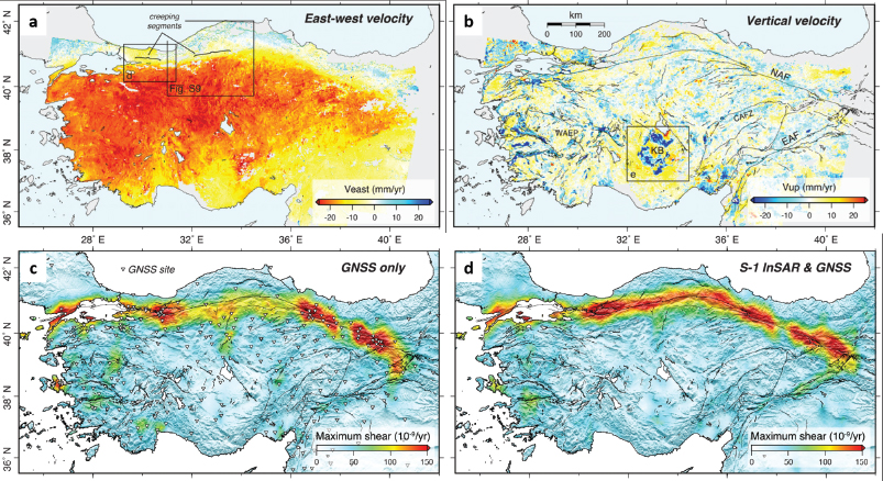
Figure 7.3. Inter-seismic deformation across Anatolia derived from Sentinel-1 InSAR and GNSS data, adapted from Weiss et al. (2020). (a) East–west velocity field derived from ascending and descending Sentinel-1 InSAR data. Boxes highlight areas of the North Anatolian Fault that are creeping. (b) Vertical velocity field. Box shows a region of significant vertical deformation due to water extraction. (c) Maximum shear strain rate estimated from GNSS only using the VELMAP approach (Wang and Wright 2012). (d) Maximum shear strain rate estimated from a combination of InSAR and GNSS data. Faults are from Emre et al. (2018). For a color version of this figure, see www.iste.co.uk/cavalie/images.zip
7.2.2.2. What have we learned about faults from InSAR studies of inter-seismic deformation
Geodetic determination of fault slip rates: for individual faults, InSAR has regularly been used to obtain estimates of their present-day slip rate (e.g. Peltzer et al. 2001; Wright et al. 2001b; Cavalié et al. 2008; Wang et al. 2009; Karimzadeh et al. 2013; Fattahi and Amelung 2016). To do so requires a few assumptions – the rheology of the seismogenic layer is typically assumed to be elastic such that strain observed in the crust away from the fault is eventually be released by slip on the fault, and the rate of strain accumulation observed geodetically is typically assumed to be representative of the long-term strain rate. If we make those assumptions, geodetic slip rates can be estimated, alongside parameters such as “locking depth” that are indicative of the seismogenic layer thickness (Wright et al. 2013). Many of the geodetic slip rates, for example on the North Anatolian and San Andreas Faults, agree with estimates from geology/paleoseismology, but in a few cases, the geodetic slip rates have disagreed with the prevailing wisdom. For example, Wright et al. (2004) used InSAR to show that the faults in western Tibet were generally accumulating strain at a slower rate than had been estimated in some geological models (e.g. Tapponnier et al. 2001). More recent geological studies have yielded Quaternary rates that are in good agreement with the geodetic rates (e.g. Cowgill et al. 2009).
Beyond the rates and styles of deformation at individual fault systems, geodetic measurements of inter-seismic strain at faults have led to new insights into fault behavior in a number of key areas. We discuss these below.
Focused strain throughout the earthquake cycle for most faults: inter-seismic deformation, particularly at strike-slip faults, is often modeled using a simple elastic rheology, in which the deep part of a fault slips at a steady rate whereas the shallow part is locked. For strike-slip faults, a screw dislocation formulation can be used (Savage and Burford 1973); other fault geometries can be modeled with a backslip formulation (Savage 1983). These elastic dislocation models give rise to relatively focused areas of inter-seismic strain around active faults; in the standard screw dislocation model, 70% of the motion for a strike-slip fault, for example, occurs within a distance of two locking depths from the fault.
Wright et al. (2013) noted that these simple elastic dislocation models were ubiquitous in studies of inter-seismic deformation; their review found 187 examples in the literature. The fact that focused strain is seen at most faults suggests that it occurs at all phases of the earthquake cycle. This argument is supported by observations of late-stage inter-seismic deformation at several major strike-slip faults that later failed in earthquakes, including the North Anatolian Fault at Izmit (Turkey), the San Andreas Fault at Parkfield (California), the Denali Fault in Alaska and the Manyi Fault in Tibet (Elliott et al. 2016). This is a somewhat surprising result – if the viscosity of the lower crust is as low as some studies of post-seismic deformation have suggested (see below), then we would not expect focused inter-seismic strain late in the earthquake cycle (e.g. Hetland and Hager 2006).
There are a few exceptions, however, where faults do not appear to have clear focused strain associated with them during the inter-seismic period. A clear recent example is from Wang et al. (2019), who used ERS and Envisat data to map inter-seismic tectonic strain across south-central Tibet. Of the five extensional grabens in their study region, only two had clear focused extensional strain in the inter-seismic geodetic velocity field.
Temporal invariance of inter-seismic strain rate: typical inter-event times for major earthquakes on large faults are hundreds to thousands of years, so modern geodetic measurements are inevitably only available for a small portion of this period. To assess whether strain rates vary throughout this time period, indirect methods are required. Meade et al. (2013) compared short-term geodetic estimates of slip rate for 15 continental strike slip faults with long-term geological estimates of slip rate, estimated over multiple earthquake cycles, finding very good agreement overall between these rates. They argued, persuasively, that because the geodetic rates sample random short intervals within the earthquake cycle, the geodetic rates must be fairly constant throughout the earthquake cycle, apart from during a relatively short post-seismic period.
Hussain et al. (2018) took a different approach to the same problem, examining present-day strain rates along the entire North Anatolian Fault from InSAR alongside estimates of strain from GPS measurements before and after the 1999 Izmit earthquakes. As major earthquakes have occurred at different times in the past, these spatial samples of strain rate can be thought of as sampling different time periods of the earthquake cycle, assuming the entire fault behaves in a similar way. They found that strain rates were approximately constant apart from an approximately 10-year period following the 1999 earthquakes (Figure 7.4). This observation requires that the relaxation time for the majority of the mid to lower crust be as long as the inter-event time (Figure 7.4; Yamasaki et al. 2014; Hussain et al. 2018).
The fact that, for large strike-slip faults at least, the inter-seismic strain rate outside the post-seismic period appears to be fairly time invariant is good news for hopes to use geodetic observations to help constrain seismic hazard models. The primary input for most modern probabilistic seismic hazard models are instrumental and historical records of previous earthquakes. These can be biased, particularly in areas of moderate to low strain, because of the relatively short observation period compared to the inter-event time (see e.g. Stein et al. 2012). If short-term geodetic strain rates really are largely representative of long-term rates of fault activity, then they have the potential to be an important dataset for constraining earthquake hazard (e.g. Bird and Kreemer 2015).
7.2.3. Post-seismic deformation and aseismic deformation transients
7.2.3.1. History and recent progress in the study of aseismic deformation transients
As geodetic data from InSAR and GNSS have shown improvements in accuracy and sampling period, it has become increasingly evident that aseismic deformation transients are an important phenomenon in fault zones. They can occur as periods of accelerated post-seismic deformation following earthquakes, when the rate of deformation is higher than the inter-seismic period (e.g. Nur and Mavko 1974), or as “slow earthquakes”, where the aseismic deformation transients are not obviously associated with the earthquake cycle (e.g. Sacks et al. 1978).
The first post-seismic studies using InSAR came just a few years after the first coseismic studies by Massonnet et al. (1996) and Peltzer et al. (1996). Although these authors studied the same earthquake, their observations were limited to just a few post-seismic interferograms and they invoked different mechanisms to explain the data. A number of studies in the 2000s presented coarsely sampled time series showing how post-seismic deformation evolved through time (e.g. Fialko 2004; Ryder et al. 2007; Biggs et al. 2009). Prior to the launch of Sentinel-1 in 2014, there were around 23 earthquakes with geodetic observations of post-seismic deformation, of which more than half had been detected by InSAR. The latest generation of InSAR missions, including Sentinel-1, allow the spatial and temporal history of post-seismic deformation to be mapped with unprecedented detail (e.g. Figure 7.5; Floyd et al. 2016; Ingleby et al. 2020; Wang and Bürgmann 2020).
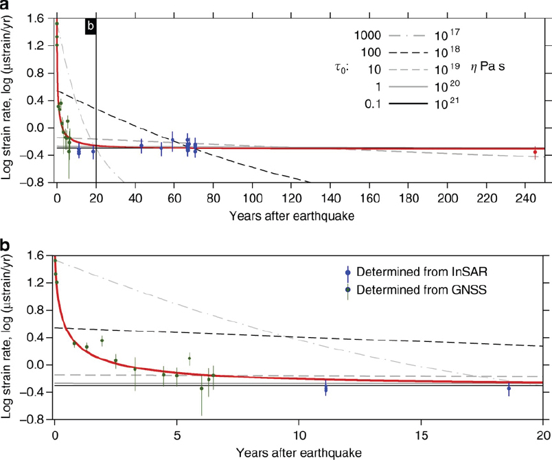
Figure 7.4. Strain rate throughout the earthquake cycle for the North Anatolian Fault, reproduced under creative commons license from Hussain et al. (2018). (a) Strain rates derived from InSAR and GNSS plotted as time since the most recent earthquake in the location of the measurement, providing a pseudo-history of the strain rate throughout a single earthquake cycle. Black lines show predictions from a simple two-layer viscoelastic coupling model (Savage and Prescott 1978), with the viscosity of the substrate shown in the legend. The red line is a best-fit model that includes post-seismic afterslip and viscoelastic relaxation embedded within a stronger substrate. (b) Magnification of the post-seismic period. For a color version of this figure, see www.iste.co.uk/cavalie/images.zip
Aseismic deformation has also been observed with InSAR. Some of the earliest InSAR observations of aseismic deformation were for creeping sections of major faults, including the Hayward and San Andreas faults in California (Bürgmann et al. 2000; Johanson and Bürgmann 2005) and the North Anatolian Fault in Turkey (Cakir et al. 2005). With more recent data it has been possible to map the spatial and temporal distribution of creep, showing that it often accrues in aseismic transient slip events (“slow earthquakes”). Furuya and Satyabala (2008) were the first to present InSAR observations of a slow earthquake, for the Chaman fault system in Afghanistan – lasting around a year and with an equivalent moment magnitude of 5.0. By using time-series analysis, several authors have now been able to map the spatial and temporal distribution of creep events at continental strike-slip faults (Rousset et al. 2016; Pousse Beltran et al. 2016; Khoshmanesh and Shirzaei 2018). Cavalié et al. (2013) presented the first observations from InSAR of a slow slip event on a subduction zone, at Guerrero, Mexico, but in general, the deformation caused by slow slip events at subduction zones has been too small to be reliably detected using InSAR.
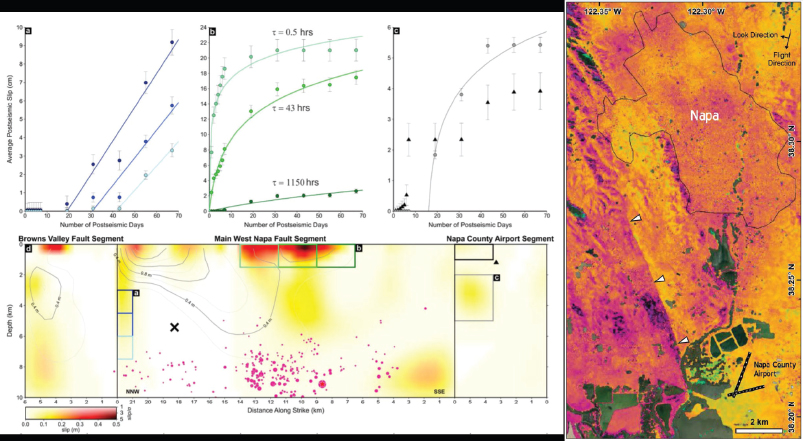
Figure 7.5. Post-seismic deformation for the 2014 South Napa earthquake, adapted from Floyd et al. (2016) and Elliott et al. (2015) Right-hand side: phase for 12-day post-seismic interferogram spanning surface rupture of the South Napa earthquake (Elliott et al. 2015). Left-hand side: (d) modeled distribution of post-seismic slip, in colors, determined from joint inversion of INSAR and GNSS time series, compared to coseismic slip contours (black contours) and aftershocks (pink circles). (a–c) Slip histories for the patches of the fault model – locations are shown in (d). For a color version of this figure, see www.iste.co.uk/cavalie/images.zip
7.2.3.2. What have we learned about faults from InSAR studies of aseismic deformation transients
Post-seismic deformation is now commonly observed: for most moderate to large earthquakes, post-seismic deformation is now routinely observed – it is now recognized as an important part of the earthquake deformation cycle. However, multiple mechanisms have been invoked to explain the observations (Wright et al. 2013), notably frictional afterslip (e.g. Floyd et al. 2016), viscoelastic relaxation (e.g. Ryder et al. 2007) and poroelastic rebound (e.g. Jónsson et al. 2003). Often, different mechanisms are invoked for the same earthquake from geodetic datasets with different time or spatial scales (Wright et al. 2013). For the 1992 Landers earthquake, post-seismic deformation has been attributed to afterslip and fault zone contraction (Massonnet et al. 1996), poroelastic deformation (Peltzer et al. 1996), deep afterslip (Savage and Svarc 1997), a combination of poroelastic deformation and deep afterslip (Fialko 2004), linear Maxwell viscoelastic relaxation of the lower crust (Deng et al. 1998) and power-law viscoelastic relaxation of the mantle (Freed and Bürgmann 2004).
Multiple processes contribute to post-seismic deformation: when looking at individual earthquakes with detailed time series of geodetic data, such as was possible for the 2014 Mw 6.1 South Napa earthquake by combining GNSS with Sentinel-1 InSAR, the spatial and temporal distribution of deformation appears as somewhat complex (Figure 7.5; Floyd et al. 2016); afterslip appears to start at different times in different locations and have different temporal decay patterns (compare the slip histories in panels (a) to (c) of Figure 7.5). To try to make sense of the complexity, Ingleby and Wright (2017) compiled time histories of post-seismic velocity for all observations of post-seismic deformation from continental earthquakes (151 velocity observations from 34 events). They showed that the maximum post-seismic velocities are inversely proportional to the time since the earthquake, like Omori’s law for aftershocks (Utsu et al. 1995). This requires frictional afterslip or a highly nonlinear viscoelastic deformation of a shear zone (Ingleby and Wright 2017). However, the maximum post-seismic velocities studied by Ingleby and Wright (2017) are likely to be dominated by shallow fault zone processes, such as afterslip. Studies of large earthquakes show that a combination of frictional afterslip and deeper viscoelastic deformation is required (e.g. Weiss et al. 2019). To separate the contributions of these mechanisms requires long time periods of precise observations over large spatial scales.
A wide range of complex aseismic phenomena occur: in addition to post-seismic deformation, InSAR has helped identify a range of complex and varied aseismic creep behavior, including triggered slip, fault creep and slow earthquakes. Triggered aseismic slip of nearby faults has been observed following a number of major earthquakes (e.g. Wright et al. 2001a; Fielding et al. 2004; Fujiwara et al. 2016). Xu et al. (2020) presented a compelling analysis of 169 fractures away from the main faults that deformed during the 2019 Ridgecrest earthquake sequence (Mw 6.4, 7.1, California). They showed that fractures that experienced coseismic stress changes that were in the same sense as the regional stress field had narrow deformation zones and were likely to have failed due to permanent inelastic deformation, such as fault slip. Faults that were stressed coseismically in the opposite sense to the regional stress had wider deformation zones, with deformation likely to be the result of enhanced strain in a compliant fault zone.
Detailed studies of time series of aseismic creep are starting to reveal complexities in the temporal behavior of creep. For example, Rousset et al. (2016) used a dense time series of high-resolution InSAR data to document a pulse of fault creep that took place over around a month in 2013. The pulse had a magnitude of 15 mm and was the only significant fault motion to occur in their observation window (July 2013 to April 2014). Similarly, Khoshmanesh et al. (2015) showed that creep at the Parkfield section of the San Andreas Fault was not steady in time, instead occurring in pulses separated by one to three years. Khoshmanesh and Shirzaei (2018) suggest that the pulsing is caused by variations in normal stress that result from pore fluids trapped in hydraulically-isolated parts of the fault.
Aseismic behavior is related to lithology: spatial maps of aseismic fault creep have been powerful in illuminating the close relationship between aseismic creep and fault zone lithology. In Taiwan, Thomas et al. (2014) showed that creep occurred on the Longitudinal Valley Fault in Taiwan in areas where fault zone gouge was dominated by a particular lithological unit, derived from unlithified subduction zone mélange, that favored pressure solution creep. In Turkey, Cetin et al. (2014) showed that creep on the North Anatolian Fault is fastest in areas where the lithology has low frictional strength, including andesitic-basaltic, limestone and serpentine units caught up in the fault zone. The relationship between aseismic deformation and lithology has also been observed in post-seismic data – regions of shallow afterslip that occurred following the 2014 South Napa earthquake correlated with younger sediments and alluvium; Floyd et al. (2016) argued that the complex variations in spatial and temporal behavior (Figure 7.5) may be a function of different clay contents, mineralogy or pore pressures within these units.
As the quality of InSAR time series improve globally, we expect to see further advances in our understanding of the aseismic behavior of faults.
7.3. Investigating earthquake surface ruptures with optical image correlation
7.3.1. A history of the optical correlation technique in the study of earthquakes
Developed for the study of earthquakes in the early 2000s, the optical correlation technique allows the retrieval of 2D or 3D ground displacements produced by an earthquake from the measurement of pixel shifts between optical images acquired before and after the event (Van Puymbroeck et al. 2000). The main advantage of this technique is the efficiency in capturing the near-fault deformation of surface-rupturing earthquakes (Mw 6.5+). Optical correlation therefore addresses one of the main limitations of the various traditional methods typically used to characterize the coseismic displacements in continental earthquakes. On the one hand, field investigations undertaken following an earthquake allow the on-fault slip at the surface to be measured from the offset of linear features displaced across the fault (e.g. roads, fences, canals and geomorphic features). However, these measurements are made only at a limited number of locations where easily recognizable features can be reliably measured across the fault, and therefore do not give a continuous representation of the surface fault slip. Moreover, the deformation is not always localized on a structurally simple fault plane, but can be expressed as a broad zone of distributed deformation that can be hundreds of meters wide. In that case, quantifying the total displacement that occurs across the entire fault zone is challenging. Finally, field investigations can provide the along-strike and vertical component of the slip but the measurement of the fault-perpendicular component is usually not possible. On the other hand, the InSAR technique allows surface displacements to be measured with very high precision (mm-scale) and at high spatial resolution. However, when the displacement gradients are too large, the interferometric phase decorrelates, leading to an incomplete description of surface displacements near the fault rupture. Moreover, this technique only measures the displacement in one direction, along the satellite line-of-sight, which is approximately oriented obliquely east–west due to the near-polar orbit of the satellites. The sensitivity to any along-track (i.e. north–south) displacement is thus limited, while combination of ascending and descending data are needed to distinguish vertical from east–west horizontal ground displacement. Finally, the GPS technique gives very precise measurements of 3D ground displacements, albeit at a very limited number of locations.
The optical correlation technique was first applied to the measurement of earthquake-related displacements by Van Puymbroeck et al. (2000), who measured the horizontal surface displacement field produced by the 1992 Mw 7.3 Landers earthquake using Satellite Pour l’Observation de la Terre (SPOT) satellite images of 10 m resolution. The east–west (EW) and north–south (NS) displacement fields they obtained clearly show the 80 km long discontinuity corresponding to the surface rupture of the Landers earthquake, demonstrating the high potential of optical correlation for the study of earthquake ruptures in large continental earthquakes. In the following years, motivated by the successful demonstration for the Landers earthquake, the method used by Van Puymbroeck et al. (2000) was applied to other surface-rupturing earthquakes, such as the Izmit (Michel and Avouac 2002), Chi-Chi (Dominguez et al. 2003) and Kashmir earthquakes (Avouac et al. 2006), using satellite images. Michel and Avouac (2006) extended the application to aerial photos, from which they resolved the displacement field for the Kickapoo step-over (part of the Landers rupture), demonstrating the potential of using historical aerial photo archives to study past surface-rupturing earthquakes. The development of easy-to-use software for optical correlation, such as COSI-Corr (Leprince et al. 2007b) and MicMac (Rosu et al. 2015), has greatly helped to establish this geodetic technique for earthquake studies. Nowadays, more and more optical data of increasing resolution are available and near-field displacements are commonly measured using optical images each time a major continental earthquake occurs. At the time of writing, the surface displacement field of about 30 earthquakes has been measured using optical correlation (e.g Zinke et al. 2014; Milliner et al. 2015; Vallage et al. 2015; Hollingsworth et al. 2017; Marchandon et al. 2018a; Barnhart et al. 2020; Delorme et al. 2020).
7.3.2. Measuring earthquake surface displacements from optical images: methodology
Optical correlation allows the measurement of the surface displacement by comparing two or more optical images spanning an earthquake. Contrary to InSAR, optical correlation is very flexible as one can correlate images acquired by different sensors (Hollingsworth et al. 2012; Marchandon et al. 2018a), with different look angles, different resolutions (although images must be resampled to a common resolution prior to correlation), and with very long temporal baselines (increasing time difference can nevertheless impact the correlation quality as surface changes accumulate). The detection threshold of the optical correlation technique is ∼1/10 of the image pixel size (Leprince et al. 2007b), which is limited by noise in the images (e.g. illumination bias; see Lacroix et al. (2019)). The choice of the images to use depends on the amplitude of the displacement signal, as well as the spatial resolution needed for the final displacement field. For large continental earthquakes (Mw > 7), medium resolution images (10–15 m; for example, Landsat 8, SPOT-1–4 and Sentinel-2) are sufficient to describe the first-order features of the rupture. However, any displacement below the detection threshold (<1–1.5 m) will not be detected and fine details of the rupture, such as small geometrical complexities or small-scale slip variations, will not be resolvable. For smaller earthquakes, or when a detailed description of the rupture is required, high-resolution images must be used (0.3–5 m, for example, SPOT-5–7, Pléiades, WorldView, Planet and aerial photos). However, medium resolution images typically have very large footprints (e.g. Sentinel-2 across-track width is 290 km), thereby allowing an entire surface rupture (potentially extending up to several 100s of kilometers in length) with only a few pairs of images (e.g. Klinger et al. 2006). In contrast, high-resolution images cover much smaller areas (e.g. Pléiades across-track width is 20 km); consequently, a large number of images are necessary to characterize the entire rupture, especially for a rupture oriented east–west (i.e. ∼perpendicular to the satellite track). Processing high-resolution images is therefore time-consuming and supplementary processing steps, such as the bundle adjustment2 of the images, are needed in order to precisely mosaic the images together with subpixel precision.
7.3.2.1. Optical image correlation: general workflow
Measuring the horizontal surface displacement field from raw optical images requires three main steps: (1) a pre-processing step during which the pre- and post- earthquake images are co-registered and orthorectified, (2) the correlation of the pre- and post-orthoimages and (3) the post-processing of the output surface displacement maps. Some optical datasets are provided in a processed format (with radiometric and geometric corrections applied), e.g. Landsat 8, and Sentinel-2. In such cases, we may proceed directly to the correlation without any pre-processing; however, any artifacts arising from the pre-processing stages cannot be easily corrected from the processed imagery (for example, DEMs used by space agencies to orthorectify images are often lower resolution than the images, which can lead to related topographic noise in the final displacement map). If datasets are provided without geometric correction, the user must pre-process the data prior to correlation. For more details about the pre-processing and the correlation steps, we refer the reader to Chapter 2 of this book as well as to the review papers by Avouac and Leprince (2015) and Hollingsworth et al. (2020).
Basic post-processing to minimize the influence of noise on the output surface displacement fields typically includes outlier removal, based either on displacements with unrealistic values, low signal-to-noise ratio, or values which differ significantly from their neighbors (e.g. Zinke et al. 2019), and various spatial smoothing operations (e.g. low-pass, median or non-local mean filtering). Non-local mean filtering, which is a spatial averaging filter with weights applied based on the similarity with each target pixel, is particularly appropriate for denoising displacements containing sharp discontinuities, such as those produced by surface-rupturing earthquakes, because it preserves sharp edges, and thus preserves fine details of the surface rupture (Buades et al. 2005). More specific corrections can be applied depending on the case, such as the removal of ramps, stripes, or undulations due to misregistration errors, charged-couple device misalignment or unknown variations of the satellite attitude. More details about these errors and their corrections can be found in section 7.3.2.3.
Several software packages are available to process optical images. The most widely used by the earthquake science community include: COSI-Corr (Co-registration of Optically Sensed Images and Correlation (Leprince et al. 2007b)), MicMac (Multi Images Correspondances par Méthodes Automatiques de Corrélation (Rosu et al. 2015)) and ASP (Ames Stereo Pipeline (Beyer et al. 2018)).
7.3.2.2. Measuring the 3D displacement field of earthquakes from stereo optical images
With the increasing number of stereo optical images available, it is now possible to measure the vertical component of the displacement in addition to the horizontal component. Three different methods can be used; all of them require pre- and post-stereo pairs of optical images3 (with enough stereoscopic information to isolate the pre- and post-earthquake topographic signal from the tectonic signal).
DEM differencing: the most straightforward technique is to (1) compute pre- and post-earthquake DEMs from pre- and post-stereo optical images, (2) orthorectify the pre- and post-images using the relevant DEMs, (3) correlate the orthorectified images to obtain the horizontal displacement field, (4) resample the pre-DEM to incorporate the horizontal displacement and (5) compute the vertical difference between the two DEMs. If the horizontal displacement is not accounted for when differencing DEMs, the resulting vertical displacement field will be overprinted by noise correlated with misregistered topography (e.g. Oskin et al. 2012). If the amount of horizontal displacement is small enough, or in areas of smooth topography, then the pre- and post-DEMs can be simply subtracted without accounting for the horizontal displacements (Kuo et al. 2019). This technique has been successfully applied to measure the 3D displacement field of several earthquakes, such as the Norcia, Hualien and Balochistan earthquakes (Barnhart et al. 2019a; Kuo et al. 2019; Delorme et al. 2020).
3D triangulation: in the second approach, the 3D location of each point before and after the earthquake is triangulated from displacement maps computed for the stereo pre- and post-event images (Avouac and Leprince 2015; Zinke et al. 2019). Let us consider two stereo pairs of optical images covering the same area: one taken before the earthquake and the second one after (Figure 7.6). One of the pre-earthquake images is defined as the primary (i.e. reference) image, and three disparity maps are computed for the primary image and the three secondary images (Figure 7.6). As stereo images are taken with off-nadir incidence angles, the pre-earthquake disparity map contains only topographic information, while the two pre-/post-earthquake disparity maps contain a combination of stereoscopic effects and ground displacements from the earthquake (Figure 7.6). Using a ray-tracing approach, the x,y and z positions at each grid location in the pre-event correlation map can be retrieved using the pre-event correlation map and the camera positions of the pre-stereo images. Similarly, the x,y and z positions of these same points after the event can be retrieved using the post-event camera positions, and the pre-/post-correlation maps. The 3D displacements are then obtained by simply differentiating the pre- and post-3D positions. An example of computing a 3D displacement field is given in section 7.3.3.2.
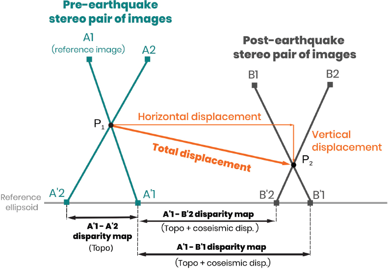
Figure 7.6. Computing the 3D displacement field from correlation of pre- and post-stereo pairs of optical images. Figure modified from Avouac and Leprince (2015). For a color version of this figure, see www.iste.co.uk/cavalie/images.zip
Point-cloud registration: finally, the third approach is to use point-cloud registration algorithms (e.g. the iterative closest point and fast global matching algorithms) on pre- and post-earthquake DEMs computed from stereo optical images. This method allows more expressive transforms to be retrieved, albeit with limited subpixel precision, thereby revealing, in the case of an affine transform, local changes in rotation, scale and shear, in addition to rigid 3D translations (e.g. Nissen et al. 2014). The advantage of using this technique instead of image correlation-based approaches is that the similarity metric is based on surface shape/morphology rather than surface reflectance. Therefore, optical images with vastly different reflectance properties (e.g. agricultural settings, regions with strong seasonal changes in vegetation and snow) are likely to fail with traditional correlation. However, if the pre- and post-event DEMs can be well-resolved for each epoch and precisely co-registered, point-cloud registration techniques can be used to retrieve the 3D ground deformation. Point-cloud registration is commonly used to measure the 3D surface deformation with LiDAR datasets (e.g. Nissen et al. 2014; Scott et al. 2018), which are generally high resolution (negating the need for subpixel performance), very high quality and well-resolved at high frequencies. This is not always the case with DEMs derived from stereo imagery, although with increasing resolution, image quality and availability of satellite and aerial datasets, and tools for processing them, this technique is finding increasing applications with optical datasets (e.g. Barnhart et al. 2019a).
7.3.2.3. Limitations and sources of error
Error and bias in surface displacement fields obtained with optical image correlation have a variety of sources. First, errors can arise from imperfect modeling of the imaging system. For example, systematic misregistration can produce a ramp over the entire displacement field. Moreover, unrecorded variations of the satellite attitude, such as pitch oscillations, can lead to across-track undulations in the displacement field (e.g. Dominguez et al. 2003; Leprince et al. 2007a), while misalignment of the charge-coupled devices (CCDs) of pushbroom sensors can cause along-track stripes (e.g. Leprince et al. 2007b). These artifacts are very common (Avouac and Leprince 2015) and can be mitigated using detrending and destriping tools (e.g. Ayoub et al. 2017). When using film-based images, unaccounted for distortions of the film (e.g. thermomechanical warping) and scanning artifacts can also bias the correlation maps (e.g. Michel and Avouac 2006; Ayoub et al. 2009). Bias affecting the entire displacement field (e.g. orbital error and film distortion) make the measurement of the absolute displacement difficult. Indeed when such errors affect the correlation, only the measured offsets across the fault are reliable whereas the absolute values of displacements are not. These errors can be mitigated by setting the far-field displacements to zero (e.g. Vallage 2015). However, when working with high-resolution images, the image coverage is too tight, so there are no zones of zero displacement. In that case, a possible solution is to work with images at different scales, anchoring high-resolution correlation with lower-resolution correlation but larger coverage. If GPS data are available, they can also be used to estimate a correction to apply to the whole optical displacement field (e.g. Dominguez et al. 2003). Topographic artifacts can appear when images are orthorectified with a lower resolution DEM, if the same DEM is used to orthorectify both pre- and post-images despite a change in topography during the earthquake, and if images are not well registered to the topography (e.g. Ayoub et al. 2009). Finally, any changes of the ground surface between the pre- and post-event images will impact the resulting displacement field. The correlation will fail in areas of drastic change, such as those due to urbanization, farming, snow, clouds or slope failure, while less drastic changes will likely be expressed as coherent noise in the correlation map. For example, if the pre- and post-images are not taken at the same time of the year, shifts in the positions of shadows between the pre- and post-acquisitions will be resolved by the correlator, leading to coherent noise in the surface displacements. This bias can be avoided by using pre- and post-images taken at the same epoch of the year (i.e. with the same illumination conditions). Alternatively, shadowing bias can also be characterized and corrected using time-series analysis (Lacroix et al. 2019; Hollingsworth et al. 2020). Indeed, because the position of the sun (i.e. azimuth and elevation) at the time of image acquisition changes throughout the year, the orientation and length of the shadows will change locally, depending on the topography. Therefore, the displacement bias induced by the shadows will be different depending on the time of the year at which the pre- and post-images were taken. By correlating all possible combinations of images taken throughout the year, the redundancy of the measurements can be used to invert a robust displacement time series for each pixel. As the time series obtained is the sum of various signals (e.g. tectonic signal + illumination bias + other noise), the isolation and removal of the illumination component can be achieved using, for example, blind source separation approaches (e.g. independent component analysis) or decomposition into known basis functions (if their functional form is known).
7.3.2.4. Perspectives and future developments
One of the main limitations of the optical correlation technique is the difficulty of measuring small displacements (cm to mm) produced by small earthquakes or by transient processes such as post-seismic deformation or inter-seismic creep (especially if the displacement signal at the surface has a long spatial wavelength). In the near future, optical images with increasing spatial and temporal resolutions will be increasingly available, along with improved correlation schemes. This large archive of optical data will thus allow measurement of displacements of increasingly smaller amplitude and with higher temporal resolution. In particular, we will be able to make use of the large archive of optical images to construct dense time series of optical displacements. Indeed, the correlation of every possible combination of optical image available between two dates will provide a set of displacement measurements with high redundancy that can be inverted for a robust time series. Time-series analysis is already used to measure small displacements using InSAR data and has started to be used with optical data to monitor slow-moving landslides and glaciers (which typically experience larger displacements compared to those produced throughout the earthquake cycle). With the increase in temporal and spatial resolution of optical imagery, we might hope that such processing methods will enable the measurements of transient deformation relating to the seismic cycle, such as post-seismic deformation or inter-seismic creep. Furthermore, machine-learning approaches applied to optical geodesy will help to improve correlator performance (faster, increased robustness and better accuracy) and may be used to detect and correct sources of noise coming from the imaging system (CCD and jitter), thereby increasing our ability to robustly measure small displacements.
7.3.3. Some examples of near-fault displacement fields from recent and historical earthquakes
In this section, we present several examples of displacement fields derived from optical data. Each example is different and is chosen for its particular methodological aspects. The first example shows how a large number of aerial images (>400) can be processed in a semi-automatic manner in order to derive a high-resolution and seamless displacement field. The second example illustrates the performance of the 3D triangulation method in retrieving the 3D displacement field of an earthquake. Finally, the third example shows how archives of historical aerial or satellite imagery can be used to study the surface rupture of past earthquakes.
7.3.3.1. Horizontal surface displacement of the 1992 Mw 7.3 Landers earthquake from high-resolution aerial images
As a first application example, we describe the horizontal displacement field of the 1992 Mw 7.2 Landers, California, earthquake measured from the correlation of aerial images. The pre-earthquake dataset was composed of ∼40 National Aerial Photography Program (NAPP) overlapping photographs of 1 m resolution acquired in July 1989 (i.e. two years before the earthquake). The post-earthquake dataset was composed of nearly 400 photographs of 20 cm resolution taken two days after the earthquake. The post-earthquake dataset was acquired specifically to map the rupture trace of the Landers earthquake and was composed of several segments of overlapping photos that follow the surface rupture (Figure 7.7). Due to the very high resolution of the images, the spatial coverage is very narrow (image width of ∼2 km, Figure 7.7). The aerial photos of each dataset were acquired with a frame camera, meaning that the incidence angle increases radially outwards from the optical center. Partially overlapping images therefore have different incidence angles and can be used to extract a DEM for the overlapping region. Therefore, for each dataset, DEMs were extracted and used to orthorectify the images. Each segment of the post-earthquake dataset was processed independently. The only metadata available for the post-images were the approximate latitude/longitude coordinates of the image center and the focal length of the camera. Therefore, using the scale of the images (estimated from several GCPs), the camera elevation was estimated and the camera information (position and orientation) refined using the bundle adjustment tool in ASP to ensure that the overlapping images were consistent with each other (i.e. to make sure that the x,y and z coordinates of features seen in several overlapping images were identical). The DEM was then extracted and registered to a reference DEM (used as ground truth) using the iterative closest point (ICP) alignment tool in ASP (“pc_align”). We used a 5 m DEM covering the entire study zone (extracted from stereo Worldview satellite images). The alignment step with the reference DEM ensured that each segment was well-registered to the same external reference and therefore consistent with neighboring segments. Once a satisfactory alignment was achieved (the alignment could be evaluated by simply differencing the aerial and reference DEMs), the aerial DEM was used to orthorectify the aerial photos. Finally, the orthoimages belonging to a given segment were mosaiced together.
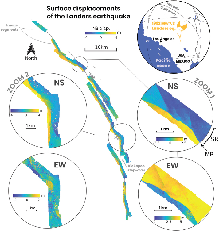
Figure 7.7. Horizontal surface displacement field of the 1992 Mw 7.3 Landers, California, earthquake. Main rupture (MR) and secondary rupture (SR) are shown, respectively. For a color version of this figure, see www.iste.co.uk/cavalie/images.zip
The same processing chain was used for the pre-earthquake images except that all images were processed simultaneously (they were all overlapping). Both the pre- and post-images were orthorectified at 1 m resolution to match the lower resolution of the pre-earthquake images. Then, the pre- and post-orthorectified images were correlated using the phase correlator of COSI-Corr with an initial window size of 64×64 pixels, a final window size of 32×32 pixels and a step size of 8 pixels. This resulted in a displacement field with ground sampling every 8 m and truly independent displacements every 32 m (although the windowing function used in the correlator resulted in nearly independent measurements every ∼16 m). Finally, measurements with a low signal-to-noise ratio (< 0.97) and outliers with displacement values higher than ± 10 m were discarded and the EW and NS displacement fields were smoothed using the non-local-mean filter implemented in COSI-Corr (Buades et al. 2005).
The surface displacement field is shown in Figure 7.7. The processing chain applied (bundle adjustment and alignment with a reference DEM) allowed a seamless horizontal displacement map to be obtained (Figure 7.7). The high-resolution displacement field allowed detection of secondary ruptures, which are clearly visible as sharp discontinuities yet were only partially mapped in the field (Figure 7.7, zoom 1). From these measurements, we can also characterize a wide zone of complex deformation that occurred north of the Kickapoo step-over (Figure 7.7, zoom 2).
7.3.3.2. Three-dimensional surface displacement of the 2016 Mw 7.8 Kaikoura earthquake from Worldview satellite images
On November 13, 2016, an Mw 7.8 earthquake struck the southeast coast of the South Island of New Zealand, 60 km southwest of the city of Kaikoura. This earthquake produced the most complex surface rupture ever observed, while the source mechanism indicated about equal thrust slip and right lateral strike-slip motion. Field investigations measured surface strike-slip up to 12 m and vertical slip up to 6.5 m. Considering the significant role that thrust faulting played in this earthquake, computation of both horizontal and vertical surface displacements was essential to sufficiently characterize the kinematics of this earthquake. Using stereoscopic Worldview 1–3 images of approximately 0.5 m resolution, Zinke et al. (2019) measured the 3D displacement field of the Kaikoura earthquake using the method describe in section 7.3.2.2 (3D triangulation approach). Before proceeding to the correlation, they first corrected sub-pixel artifacts in the raw images (from CDD array mis-alignments) using ASP. Then, for each overlapping pair of preand post-stereo images, the pre-earthquake image with an incidence angle closest to nadir was selected as the primary (to maximize the correlation with the three other images). Then, the three secondary images were coregistered to the master pre-images, and the four images were orthorectified using a coarse DEM (8 m) to remove the long-wavelength topographic distortions (thus allowing the remaining high-frequency stereoscopic distortions to be retrieved with a relatively small 32×32 correlation window). Then, the primary image was correlated with the three secondary images to compute disparity maps that contained information on both the short-wavelength (<8 m) topographic distortions and the tectonic displacement. Finally, they used a ray tracing approach between the disparity maps and satellite position to obtain the pre- and post-event 3D positions of each point of the ground. The 3D displacement was then obtained by simply differentiating the pre- and post-3D positions of each point of the ground (Zinke et al. 2019). ICP alignment was then used to align each correlation map with its neighbor, and the full displacement map was then aligned to either an independent correlation map (e.g. derived from correlation of Landsat 8 images) or GPS data.
The 3D displacement field of the Kaikoura earthquake is shown in Figure 7.8 and highlights a very geometrically and kinematically complex rupture composed of 19 faults, including one fault previously unmapped structure, the Snowflake Spur fault (Zinke et al. 2019). The surface slip amplitude is highly variable, with significantly larger slip in the northern region, where the slip is subparallel to the plate motion direction, than in the southern part, where the slip is subperpendicular to the plate motion direction (Figure 7.8).
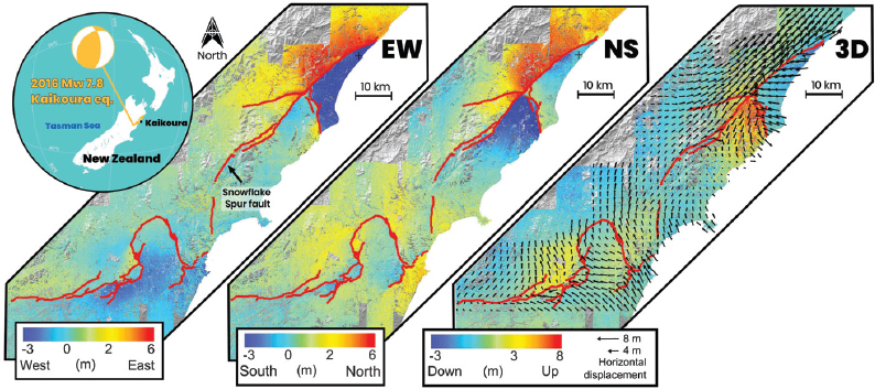
Figure 7.8. Three-dimensional surface displacement field of the 2016 Mw 7.8 Kaikoura, New Zealand, earthquake processed by Zinke et al. (2019). Red lines highlight the complex surface rupture trace. For a color version of this figure, see www.iste.co.uk/cavalie/images.zip
7.3.3.3. Horizontal surface displacement field of the 1979 Mw 7.1 Khuli-Boniabad, Iran, earthquake from KH-9 spy satellite images
The optical image correlation technique allows us to take advantage of the substantial archive of historical aerial and satellite images to document the surface displacement fields of past earthquakes. The oldest events that have currently been studied with optical data occurred in 1975–1984 (Krafla seismo-volcanic rifting crisis crisis (Hollingsworth et al. 2012, 2013)), 1978 (Tabas earthquake (Zhou et al. 2016)) and 1979 (Khuli-Boniabad earthquake (Marchandon et al. 2018a)); nevertheless, any earthquake can be studied for which pre-imagery exists, potentially extending as far back as the beginning of aerial photography in the early 20th century. Correlation of aerial photos therefore provides a powerful method to considerably increase the database of documented surface ruptures, which are important for fault mechanics and seismic hazard research (as in the SURE database). For this purpose, the declassified KH-9 US spy satellite images are particularly useful. The KH-9 spy satellite was active between 1973 and 1980 and acquired ∼29,000 images globally with a footprint of 250×125 km and a resolution of 6–9 m. The KH-9 negatives are scanned by the USGS at 7 µm (3,600 dpi) using a high-performance photogrammetric film scanner, and the digital copies can be purchased from the USGS Earth Explorer website for USD 30. Although KH-9 image metadata have not been declassified, KH-9 images were acquired with a camera similar to the Large Format Camera (LFC) used by NASA in 1984, which featured a 23×46 cm frame camera with a focal length of 30.5 cm. For the purposes of orthorectification, they can be treated as very high altitude aerial photos (Surazakov and Aizen 2010; Hollingsworth et al. 2012). In the example presented in this section, the surface displacement field of the 1979 Mw 7.1 Khuli-Boniabad, Iran, earthquake was measured using a KH-9 pre-earthquake image and a 10 m Sentinel-2 post-earthquake image (Marchandon et al. 2018a; Figure 7.9). A Sentinel-2 image taken in the same season (i.e. January) as the KH-9 image was used to limit the illumination bias in the correlation (Hollingsworth et al. 2017; see also section 7.3.2.3). Using the COSI-Corr software package, the KH-9 image was coregistered and orthorectified using the post-earthquake Sentinel-2 image as reference and a 0.5 m resolution Pléiades-derived DEM of the studied area. A very long-wavelength trend was removed from both components of the EW and NS displacement fields by subtracting a second-order polynomial using the detrending tool of COSI-Corr. Such distortions are commonly seen when correlating film-based images and are usually due to thermo-mechanical warping of the photographic film (Michel and Avouac 2006). Nevertheless, the sharp discontinuity associated with the rupture was unaffected by long-wavelength denoising.
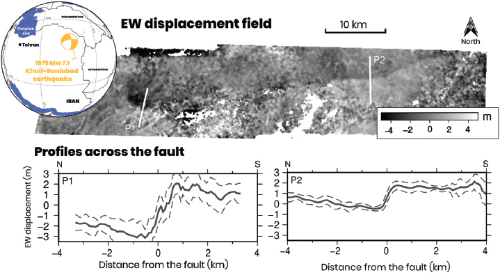
Figure 7.9. EW surface displacement field and profiles across the fault of the 1979 Mw 7.1 Khuli-Boniabad, Iran, earthquake processed by Marchandon et al. (2018a). For a color version of this figure, see www.iste.co.uk/cavalie/images.zip
The left-lateral surface rupture trace is clearly visible on the EW displacement field (Figure 7.9). The 50-km long rupture trace trends ∼N70°, before bending abruptly N160° (west of point F) at its western termination. Surface displacements in the western part of the rupture (west of point F) are typically higher than in the eastern part of the rupture (between points B and C). This is shown by the two example profiles P1 and P2, which reveal fault offsets of ∼ 4.92 ± 0.73 m and ∼ 2.24 ± 0.26 m.
7.3.4. New insights from high-resolution near-fault displacement maps
Optical correlation has revolutionized the characterization of surface ruptures of large continental earthquakes. Using surface displacement maps derived from optical correlation, the geometry of the surface rupture and along-strike slip variability can be easily quantified, typically much more quickly than field-based approaches, particularly in remote regions. In addition to enabling an efficient characterization of the surface rupture, these data can be used in a variety of ways to increase our understanding of earthquakes. The principal ones are described in the following sections.
7.3.4.1. Characterization of off-fault deformation
During an earthquake, a fraction of the coseismic strain is released off the main fault, either as localized slip on minor secondary faults or as inelastic deformation expressed as warping, granular flow or rigid-block rotation (Figure 7.10; Nelson and Jones 1987; Shelef and Oskin 2010). Given its nature, coseismic distributed deformation is difficult to observe and quantify during field surveys. Indeed, field offset measurements are typically made within 10 m of the primary fault strand and thus capture only the on-fault component of the deformation. Some field studies have also attempted to capture the coseismic distributed deformation. For example, Rockwell et al. (2002) used linear features crossing the fault (e.g. tree alignment, fences, walls or canals) to measure deformation accommodated off the main fault by inelastic processes during the 1999 ˙Izmit and Düzce earthquakes. They found that up to 40% of the total slip was accommodated off the primary fault plane over lateral distances up to 100 m. The same approach can be taken with visual inspection of high-resolution optical images (e.g. Zinke et al. 2014; Gold et al. 2015). However, estimation of off-fault deformation in this way can be time-consuming and interpretive and may only be achieved in areas where long linear features cross the fault.
By capturing the pattern of near-field deformation, optical correlation allows measurement of the total shear accommodated across the fault at high spatial resolution. Optical displacement fields can thus be used to characterize the off-fault deformation (e.g. magnitude, spatial distribution and width) in recent surface-rupturing earthquakes, and to evaluate which parameters control its characteristics (e.g. Zinke et al. 2014, 2019; Milliner et al. 2015; Vallage et al. 2015). The total surface slip accommodated across the fault zone, along with the width over which it is accommodated, are usually measured from fault-perpendicular stacked profiles spaced regularly along the fault strike (e.g. Zinke et al. 2014; Milliner et al. 2015). On each side of the displacement profile, a linear regression is fitted from the far-field to the point where the displacement profile shows an inflection near the fault (care must be taken to account for any near-fault artifacts introduced by smoothing operations, as well as correlated noise). Then, the linear regressions are extrapolated to the fault trace and the relative difference between the extrapolated regressions defines the offset across the entire fault zone, while the distance between the inflection points located each side of the fault defines the fault zone width (Figure 7.10). The amount of off-fault deformation is then quantified by subtracting the on-fault slip (e.g. offsets measured in the field) from the total slip measured from optical displacement maps (i.e. total slip across the entire fault zone), and expressed as a percentage of the total slip. The method relies on the assumption that the differences between optical and on-fault offsets reflect only the degree of optical frequency division (OFD) and not a reduction of localized slip on the primary fault plane in the uppermost tens of meters of the crust. A comparison between the along-strike offsets measured from optical displacement maps and those measured within a few meters of the main fault strand (by inspection of satellite imagery) of the 2013 Mw 7.7 Balochistan earthquake (Zinke et al. 2014) is shown in Figure 7.11.
The average amount of off-fault deformation inferred from high-resolution near-fault displacement fields for various earthquakes ranges from 20% to 60%, while the mean fault-zone width ranges from ∼100 to ∼400 m (Zinke et al. 2014; Gold et al. 2015; Milliner et al. 2015; Kuo et al. 2019; Scott et al. 2018; Zinke et al. 2019). It should be noted, however, that the data and method used to estimate OFD can provide significantly different results for a given earthquake (e.g. 45% vs. 28% for the Balochistan earthquake in Zinke et al. (2014) and Gold et al. (2015), respectively). The parameters controlling the amount of OFD from one rupture to another are not completely understood, although fault zone maturity is thought to play a significant role: with increasing fault maturity (e.g. increasing cumulative offset, see Manighetti et al. (2007)), the fault becomes geometrically smoother (Brodsky et al. 2011), while developing wider and more enhanced damage zones (Faulkner et al. 2011) and more established (and mechanically weak) gouge zones, ultimately leading to increased localization of slip during an earthquake (Dolan and Haravitch 2014; Socquet et al. 2019). Cumulative long-term OFD has also been estimated using long-term markers of deformation; for example, Salyards et al. (1992) measured the paleomagnetic rotation of sediments at a site on the San Andreas fault and found that as much as 78% of the deformation was distributed over a fault zone width of ∼45 m. Shelef and Oskin (2010) used geologic features (i.e. dikes and inactive faults) offset by active strike-slip faults in the Eastern California Shear Zone to conclude that distributed displacement accommodates up to 25% of the total displacement within 100–200 m of the studied faults; such values are also consistent with coseismic estimates from a structurally mature section of the 2016 Kaikoura earthquake (Zinke et al. 2019), with occurring within ∼100 m of the fault zone.
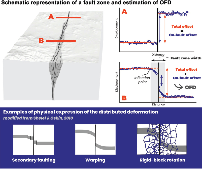
Figure 7.10. Schematic representation of the distribution of deformation within a fault zone. For a color version of this figure, see www.iste.co.uk/cavalie/images.zip
Along the length of a surface rupture, the amount of OFD can vary significantly, with OFD ranging from 0% (deformation entirely localized at the primary fault core) to 100% (completely distributed deformation). However, on average, the deformation is more localized at structurally simple sections of the fault and more distributed at structurally complex ones. For example, for the 2013 Mw 7.7 Balochistan earthquake, the percentage of OFD was 26% for structurally simple segments of the rupture, and 56% for structurally complex segments (Zinke et al. 2014). Similarly, the mean amount of OFD for the 1992 Mw 7.2 Landers earthquake was 15% in structurally simple parts of the fault and 50% in structurally complex parts of the fault (Milliner et al. 2015).
The type of near-fault materials also seems to control the amount of OFD. For the Balochistan earthquake, Zinke et al. (2014) found a general tendency for the deformation to be more distributed in younger and thicker sediments, although the trend was weak. Similarly, for the Hector-Mine earthquake, Milliner et al. (2016a) found larger OFD where the rupture propagated through sediments compared with bedrock ( ∼40% vs. 20%). This observation is not systematic however. For the Landers earthquake, Milliner et al. (2015) found similar and large ranges of OFD in areas of sediment–sediment and basement–basement interfaces (mean of ![]() and
and ![]() respectively) and lower OFD (mean of 20%) in areas with a strong bimaterial interface (i.e. where the fault juxtaposes bedrock against sediment). Lower amounts of OFD on bimaterial interfaces has also been observed for the 2018 Mw 7.5 Palu earthquake (Socquet et al. 2019) and likely results from enhanced localization along the strong contrast in material rigidity (Andrews and Ben-Zion 1997).
respectively) and lower OFD (mean of 20%) in areas with a strong bimaterial interface (i.e. where the fault juxtaposes bedrock against sediment). Lower amounts of OFD on bimaterial interfaces has also been observed for the 2018 Mw 7.5 Palu earthquake (Socquet et al. 2019) and likely results from enhanced localization along the strong contrast in material rigidity (Andrews and Ben-Zion 1997).
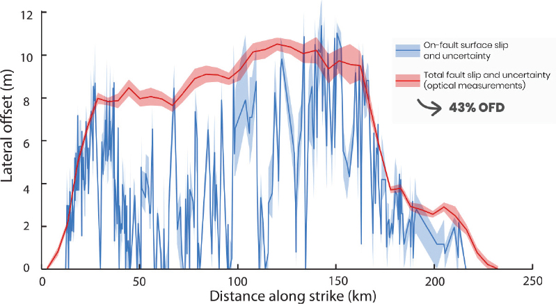
Figure 7.11. Comparison of the along-strike offsets measured on the main fault strand (blue) and across the entire fault zone (red, optical offsets) for the 2013 Mw 7.7 Balochistan earthquake (modified from Zinke et al. (2014)). For a color version of this figure, see www.iste.co.uk/cavalie/images.zip
Finally, the amount of OFD can be impacted by the local topography. Weaker sediments tend to dominate the surface geology in flat and low-lying areas (e.g. flood plains), while steep mountainous regions often feature strong bedrock materials; therefore, we may expect to see more OFD where fault ruptures cross flat, sediment-filled areas, and less OFD in mountainous settings. Nevertheless, Zinke et al. (2019) found the opposite (albeit relatively weak) relationship along the Kekerengu segment of the 2016 Mw 7.8 Kaikorua earthquake, with more OFD in the steep mountains compared to the low-slope coastal regions. One explanation proposed by Zinke et al. (2019) is topographic amplification of SH seismic waves, which could in turn enhance the damage within the fault zone, especially where it intersects the surface (e.g. Boore 1972; Ma 2008). Delorme et al. (2020) also noted the influence of topography on surface slip following the 2016 Norcia earthquake (normal), which featured locally enhanced (i.e. very shallow) slip on the primary fault plane along steep sections of the fault. Hollingsworth et al. (2019) also noted that low slope regions generally featured more OFD compared with steep slope regions for the Norcia event, with the steepest slopes featuring locally enhanced slip (shallow slip surplus). Gravitational effects have been postulated as a contributing factor for locally enhancing the slip where the fault breaks the surface (Delorme et al. 2020).
High-resolution optical displacement fields can also be used to infer surface strain tensors (e.g. Scott et al. 2018; Barnhart et al. 2020). The zone of inelastic failure can be readily observed by delineating the areas where the threshold between elastic and inelastic strain is exceeded (a ratio of 0.5% is commonly assumed for surface materials; for example, Scott et al. (2018). In a recent study, Barnhart et al. (2020) inferred the surface-strain tensors of the 2019 Mw 7.1 Ridgecrest, California, earthquake and showed that the zone of inelastic deformation inferred from the shear strain tensor (where the 0.5% threshold was exceeded) was narrow (width of ∼25 m) and did not correlate with the width of off-fault deformation inferred from fault-perpendicular profiles ( ∼63 m). Furthermore, they showed that the width inferred from the strain tensors was consistent along the rupture compared to the OFD width, which was much more variable. They also showed that no correlation exists between the inelastic failure width and the near-fault materials. According to the authors, the inelastic failure width is influenced by the fault maturity (increasing width with maturity) and by the rupture speed (narrower width with increasing rupture speed).
Understanding the degree to which the deformation is localized within the fault zones has several important implications. First, if the deformation is distributed within hundreds of meters from the main fault trace, fault slip rates deduced from measurements of offset geological markers made within tens of meters of the main fault trace could be significantly underestimated (Dolan and Haravitch 2014). If real, this underestimation has several consequences. First, the estimation of seismic hazard using probabilistic approaches incorporating geological fault slip rates could lead to a systematic underestimation of the real hazard. Second, any interpretation of the differences observed between geological slip rate and geodetic loading rate would be biased. The degree to which the deformation is localized can also influence the frequency content and magnitude of strong ground motions during an earthquake (Dolan and Haravitch 2014). Better understanding the link between off-fault deformation and strong ground motion could therefore help to make more accurate predictions of strong ground motions in future earthquakes and thus better assess seismic hazard. Finally, partitioning of slip into damage zones has major implications for how we interpret information recorded in paleoseismic trenches, as offset markers only capture a component of the slip at depth, and may thus lead to an incorrect estimate of past earthquake magnitudes, which also form an integral part of seismic hazard assessment.
High-resolution optical maps of coseismic surface displacements can also be combined with dynamic rupture modeling incorporating off-fault damage to determine the most likely rupture scenario for an earthquake. Indeed, by comparing the pattern of off-fault damage observed in the optical displacement maps with the one simulated by the dynamic rupture modeling, Klinger et al. (2018) succeeded in determining the most likely rupture scenario at the Jordan–Kekerengu–Papatea triple junction during the 2016 Mw 7.8 Kaikoura earthquake.
7.3.4.2. Improvement of fault slip model
Over the last 40 years, fault slip distribution models are routinely inferred each time a significant earthquake occurs. As the estimation of fault slip from surface data is a fundamentally ill-posed problem, slip models for a given earthquake can be very different depending on the type and quantity of data, the inversion method and the assumed fault geometry and Earth model. In the last three decades, the development of space-based geodetic techniques, in particular InSAR, has given access to increasingly complete descriptions of earthquake surface displacements, thereby increasing the robustness of slip models. However, InSAR does not routinely provide near-fault measurements for large surface-rupturing earthquakes. By improving the near-fault coverage, optical correlation data can increase the reliability of fault slip models (e.g. Dominguez et al. 2003; Xu et al. 2016; Gombert et al. 2017; Marchandon et al. 2018b; Delorme et al. 2020; Lauer et al. 2020). For example, by re-estimating the slip model of the 1997 Mw 7.2 Zirkuh earthquake, Marchandon et al. (2018b) have shown that the addition of near-field optical data in the modeling changes the obtained fault geometry, the slip amplitude and the slip distribution significantly compared to the slip model based on InSAR data only.
Furthermore, near-fault optical data have been used to better understand the origin of the shallow slip deficit (SSD) commonly seen in fault slip models for large continental strike-slip earthquakes (Fialko et al. 2005). By reassessing the fault slip model of three large strike-slip earthquakes and incorporating near-field displacements from optical correlation data, Xu et al. (2016) have shown that a significant part of the previously inferred SSD for each event was an artifact due to a lack of near-fault coverage. The impact of the lack of near-fault coverage for SSD has also been shown by Lauer et al. (2020) for the Balochistan earthquake and by Marchandon et al. (2021) using synthetic tests. However, because optical data are typically much noisier compared to InSAR, noise-related model uncertainties should be systematically estimated when using optical data in fault slip inversions in order to avoid any misinterpretations of the inferred slip models, in particular concerning the distribution of slip with depth (Marchandon et al. 2021).
7.3.4.3. Impact of the fault structural properties on the coseismic slip distribution
It has long been noticed that fault complexities can impact rupture propagation during an earthquake (King and Nabelek 1985). This impact is reflected in the coseismic slip distribution of earthquakes and shows that fault complexities such as step-overs or bends correlate with (1) zones of low slip amplitude (e.g. Lasserre et al. 2005) and (2) the start and endpoint of ruptures (e.g. King and Nabelek 1985). By providing the geometry of the surface rupture and the distribution of surface fault slip, optical correlation results have helped to increase the number of examples that illustrate the impact of fault geometry on coseismic slip (e.g. Klinger et al. 2006; Milliner et al. 2015; Vallage et al. 2015). For example, analysis of the surface coseismic slip distributions of the Khuli-Boniabad and Zirkuh earthquakes obtained from optical correlation have shown that the ruptures of these earthquakes are characterized by several segments, with the inter-segments located in zones of large-scale structural complexity of the Dasht-e-Bayaz and Abiz faults (Marchandon et al. 2018a, 2018b).
Furthermore, high-resolution optical measurements allow a more in-depth analysis of the surface slip variability. In particular, the frequency content of surface coseismic slip distributions can be analyzed by computing the power spectral density of surface slip (e.g. Milliner et al. 2016; Bruhat et al. 2020). Power spectral density (PSD) is the measure of the power content of a signal versus frequency and can be used to characterize fractal properties of a signal. By computing the PSD of the surface slip distribution of various earthquakes, it has been shown that the surface slip distribution is fractal (Milliner et al. 2016; Bruhat et al. 2020) (i.e. a power law describes the relationship between the slip amplitude and the spatial wavelength). The fractal nature of surface slip echoes the fractal nature of fault surfaces. Indeed, although faults are typically treated as planes, faults are in reality irregular surfaces at all scales (e.g. Candela et al. 2012). Dynamic rupture simulations have shown that these geometric irregularities, i.e. roughness, induce local stress perturbations that affect the rupture prorogation (e.g. rapid accelerations and decelerations of the rupture front, variability in moment release and super-shear transitions) and induce slip heterogeneities (e.g. Dieterich and Smith 2009). By analyzing the coseismic slip variability of real earthquakes, it could thus be, in principle, possible to investigate the roughness properties of the faults with which they occurred. Bruhat et al. (2020) made a first attempt towards this goal. Using a catalog containing thousands of dynamic rupture simulations on a self-similar fractal fault (H=1) with varying roughness, they investigated the relationship between the fault roughness and the spectral characteristics of the resulting slip distribution. They found that the slip distribution deviates from self-similarity (Hurst coefficient decreases) with increasing fault roughness. They also analyzed the spectral characteristics of various real earthquakes and found that the real slip distributions were significantly more self-affine (lower Hurst coefficient) compared to the simulated slip distributions, thus making it hard to draw any conclusions about the fault roughness with which these real earthquakes occurred.
7.4. Conclusion
In recent decades, the development of InSAR and optical correlation, as well as the tremendous increase of SAR and optical satellite data available, has revolutionized the measurement of surface displacements induced by the earthquake deformation cycle. Far from being interchangeable, these two methods are highly complementary, as each technique addresses the limitations of the other (see Table 11.1 for a summary of the pros and cons of each method). For nearly 30 years, InSAR measurements of coseismic deformation have contributed to showing that fault ruptures are complex (e.g. multi-segmented) and that the structural complexities of faults can sometimes impact the propagation and arrest of ruptures. Furthermore, by constraining fault slip models, InSAR data have shown that the surface slip seems to be a poor indicator of the amount of slip at depth, implying that seismic hazard estimated from geological surface offsets could be systematically underestimated. More recently, InSAR coseismic observations have been complemented by near-fault optical correlation data, which have allowed a more direct observation of the surface rupture and surface fault slip. The inclusion of near-field data from optical correlation indicate that the discrepancy between the surface slip and slip at depth previously inferred using InSAR data alone could partly be a modeling artifact, further complicated by slip being accommodated by distributed deformation in the upper crustal volume surrounding the fault (among other processes), which is not taken into account in the slip inversion. Moreover optical data have also been used to investigate the fractal properties of faults, offering a new insights into fault mechanics and generation of strong ground motions.
In contrast to optical correlation, InSAR is very efficient in measuring small displacements. The capacity of InSAR to detect small displacements has been exploited to measure inter-seismic strain rates and deduce geodetic slip rates. The comparison of short-term geodetic and long-term geological slip rates for a number of major faults suggests that the inter-seismic strain rate varies little with time, implying that it could be used to constrain seismic hazard models. Finally, InSAR data have been widely used to measure transient aseismic deformation such as post-seismic deformation and inter-seismic fault creep. Thanks to InSAR studies, we now know that post-seismic deformation is commonly observed after moderate to large earthquakes. Modeling of the post-seismic response shows that multiple post-seismic mechanisms are often required to explain the observations (e.g. afterslip, viscoelastic relaxation and poro-elastic rebound), as well as placing of constraints on the frictional properties of faults and the rheology of the lithosphere. Finally, detailed studies of transient aseismic creep have highlighted the link between fault creep and fault zone lithology and the control of pore fluid pressures on the temporal variations of creep.
Table 7.1. Summary of pros and cons of InSAR and optical correlation
InSAR Pros:
Cons:
|
Optical correlation Pros:
Cons:
|
In the future, the quality and quantity of SAR and optical images will continue to improve. Regarding the optical data, this increase associated with more effective processing methods will enable the measurement of small transient deformations. The analysis of future surface-rupturing earthquakes with optical data will also allow a more comprehensive understanding of the parameters controlling the distribution of deformation in the upper crust. Optical data can also provide constraints on models of dynamic rupture propagation incorporating off-fault deformation, which will further our understanding of how the upper crust behaves during an earthquake. Concerning InSAR, the processing of the huge Sentinel-1 data will shortly provide continent-scale maps of inter-seismic velocity. Future satellite missions, such as the L-band NISAR mission, will improve coverage and coherence, and there is the prospect of measuring 3D deformation using companion satellites of Sentinel-1. Automatic processing systems will mean that non-expert users can work with the data, and in the near future, we will begin to see inter-seismic deformation data from InSAR incorporated routinely into seismic hazard models. Collectively, the knowledge on earthquake and fault systems brought by InSAR and optical data (e.g. control of structural complexities in the rupture propagation, degree of localization of the deformation around faults in the upper crust and strain accumulation) is of great significance to both science and society and will ultimately lead to a seismically more resilient world through improved seismic hazard assessment.
7.5. Acknowledgments
The authors thank Yann Klinger for his careful reviews and comments that helped to improve this chapter.
7.6. References
Agram, P., Jolivet, R., Riel, B., Lin, Y., Simons, M., Hetland, E., Doin, M.-P., Lasserre, C. (2013). New radar interferometric time series analysis toolbox released. Eos, Transactions of the American Geophysical Union, 94(7), 69–70.
Andrews, D.J. and Ben-Zion, Y. (1997). Wrinkle-like slip pulse on a fault between different materials. Journal of Geophysical Research: Solid Earth, 102(B1), 553–571.
Attema, E., Desnos, Y.-L., Duchossois, G. (2000). Synthetic aperture radar in Europe: ERS, Envisat, and beyond. Johns Hopkins APL Technical Digest, 21(1), 155–161.
Avouac, J.-P. and Leprince, S. (2015). Geodetic imaging using optical systems. Geodesy, 3, 387–424
Avouac, J.-P., Ayoub, F., Leprince, S., Konca, O., Helmberger, D.V. (2006). The 2005, Mw 7.6 Kashmir earthquake: Sub-pixel correlation of ASTER images and seismic waveforms analysis. Earth and Planetary Science Letters, 249(3–4), 514–528.
Ayoub, F., Leprince, S., Avouac, J.-P. (2009). Co-registration and correlation of aerial photographs for ground deformation measurements. ISPRS Journal of Photogrammetry and Remote Sensing, 64(6), 551–560.
Ayoub, F., Leprince, S., Avouac, J.-P. (2017). User’s Guide to COSI-CORR Co-registration of Optically Sensed Images and Correlation. Technical report, California Institute of Technology, CA.
Barnhart, W.D., Gold, R.D., Shea, H.N., Peterson, K.E., Briggs, R.W., Harbor, D.J. (2019a). Vertical coseismic offsets derived from high-resolution stereogrammetric DSM differencing: The 2013 Baluchistan, Pakistan earthquake. Journal of Geophysical Research: Solid Earth, 124(6), 6039–6055.
Barnhart, W.D., Hayes, G.P., Wald, D.J. (2019b). Global earthquake response with imaging geodesy: Recent examples from the USGS NEIC. Remote Sensing, 11(11), 1357.
Barnhart, W.D., Gold, R.D., Hollingsworth, J. (2020). Localized fault-zone dilatancy and surface inelasticity of the 2019 Ridgecrest earthquakes. Nature Geoscience, 13(10), 699–704.
Barrick, D.E. and Swift, C.T. (1980). The Seasat microwave instruments in historical perspective. IEEE Journal of Oceanic Engineering, 5(2), 74–79.
Bekaert, D.P., Karim, M., Linick, J.P., Hua, H., Sangha, S., Lucas, M., Malarout, N., Agram, P.S., Pan, L., Owen, S.E., Lai-Norling, J. (2019). Development of open-access standardized InSAR Displacement Products by the Advanced Rapid Imaging and Analysis (ARIA) project for natural hazards. AGU Fall Meeting, G23A–04.
Beyer, R.A., Alexandrov, O., McMichael, S. (2018). The Ames stereo pipeline: NASA’s open source software for deriving and processing terrain data. Earth and Space Science, 5(9), 537–548.
Biggs, J., Burgmann, R., Freymueller, J.T., Lu, Z., Parsons, B., Ryder, I., Schmalzle, G., Wright, T. (2009). The postseismic response to the 2002 M 7.9 Denali Fault earthquake: Constraints from InSAR 2003–2005. Geophysical Journal International, 176(2), 353–367.
Bird, P. and Kreemer, C. (2015). Revised tectonic forecast of global shallow seismicity based on version 2.1 of the Global Strain Rate Map. Bulletin of the Seismological Society of America, 105(1), 152–166.
Boore, D.M. (1972). A note on the effect of simple topography on seismic SH waves. Bulletin of the Seismological Society of America, 62(1), 275–284.
Brodsky, E.E., Gilchrist, J.J., Sagy, A., Collettini, C. (2011). Faults smooth gradually as a function of slip. Earth and Planetary Science Letters, 302(1–2), 185–193.
Bruhat, L., Klinger, Y., Vallage, A., Dunham, E.M. (2020). Influence of fault roughness on surface displacement: From numerical simulations to coseismic slip distributions. Geophysical Journal International, 220(3), 1857–1877.
Buades, A., Coll, B., Morel, J.-M. (2005). A non-local algorithm for image denoising. IEEE Computer Society Conference on Computer Vision and Pattern Recognition (CVPR’05), 60–65.
Bürgmann, R., Schmidt, D., Nadeau, R., d’Alessio, M., Fielding, E., Manaker, D., McEvilly, T., Murray, M. (2000). Earthquake potential along the northern Hayward fault, California. Science, 289(5482), 1178–1182.
Cakir, Z., Akoğlu, A.M., Belabbes, S., Ergintav, S., Meghraoui, M. (2005). Creeping along the Ismetpasa section of the North Anatolian fault (Western Turkey): Rate and extent from InSAR. Earth and Planetary Science Letters, 238(1–2), 225–234.
Cakir, Z., Ergintav, S., Akoğlu, A.M., Çakmak, R., Tatar, O., Meghraoui, M. (2014). InSAR velocity field across the North Anatolian Fault (eastern Turkey): Implications for the loading and release of interseismic strain accumulation. Journal of Geophysical Research: Solid Earth, 119(10), 7934–7943.
Candela, T., Renard, F., Klinger, Y., Mair, K., Schmittbuhl, J., Brodsky, E.E. (2012). Roughness of fault surfaces over nine decades of length scales. Journal of Geophysical Research: Solid Earth, 117(B8), 1–30.
Cavalié, O., Lasserre, C., Doin, M.-P., Peltzer, G., Sun, J., Xu, X., Shen, Z.-K. (2008). Measurement of interseismic strain across the Haiyuan fault (Gansu, China), by InSAR. Earth and Planetary Science Letters, 275(3–4), 246–257.
Cavalié, O., Pathier, E., Radiguet, M., Vergnolle, M., Cotte, N., Walpersdorf, A., Kostoglodov, V., Cotton, F. (2013). Slow slip event in the Mexican subduction zone: Evidence of shallower slip in the Guerrero seismic gap for the 2006 event revealed by the joint inversion of InSAR and GPS data. Earth and Planetary Science Letters, 367, 52–60.
Cetin, E., Cakir, Z., Meghraoui, M., Ergintav, S., Akoglu, A.M. (2014). Extent and distribution of aseismic slip on the Ismetpa¸sa segment of the North Anatolian Fault (Turkey) from persistent scatterer InSAR. Geochemistry, Geophysics, Geosystems, 15(7), 2883–2894.
Cowgill, E., Gold, R.D., Xuanhua, C., Xiao-Feng, W., Arrowsmith, J.R., Southon, J. (2009). Low Quaternary slip rate reconciles geodetic and geologic rates along the Altyn Tagh fault, northwestern Tibet. Geology, 37(7), 647–650.
Delorme, A., Grandin, R., Klinger, Y., Pierrot-Deseilligny, M., Feuillet, N., Jacques, E., Rupnik, E., Morishita, Y. (2020). Complex deformation at shallow depth during the 30 October 2016 Mw6. 5 Norcia earthquake: Interference between tectonic and gravity processes? Tectonics, 39(2), e2019TC005596.
Deng, J., Gurnis, M., Kanamori, H., Hauksson, E. (1998). Viscoelastic flow in the lower crust after the 1992 Landers, California, earthquake. Science, 282(5394), 1689–1692.
Dieterich, J.H. and Smith, D.E. (2009). Nonplanar faults: Mechanics of slip and off-fault damage. Pure Applied Geophysics, 166, 1799–1815.
Doin, M.-P., Guillaso, S., Jolivet, R., Lasserre, C., Lodge, F., Ducret, G., Grandin, R. (2011). Presentation of the small baseline NSBAS processing chain on a case example: The Etna deformation monitoring from 2003 to 2010 using Envisat data. ESA SP-697 Fringe Symposium, Frascati.
Dolan, J.F. and Haravitch, B.D. (2014). How well do surface slip measurements track slip at depth in large strike-slip earthquakes? The importance of fault structural maturity in controlling on-fault slip versus off-fault surface deformation. Earth and Planetary Science Letters, 388, 38–47.
Dominguez, S., Avouac, J.-P., Michel, R. (2003). Horizontal coseismic deformation of the 1999 Chi-Chi earthquake measured from SPOT satellite images: Implications for the seismic cycle along the western foothills of central Taiwan. Journal of Geophysical Research, 108(B2), 1–19.
Ekström, G., Stein, R.S., Eaton, J., Eberhart-Phillips, D. (1992). Seismicity and geometry of a 110-km-long blind thrust fault 1. The 1985 Kettleman Hills, California, earthquake. Journal of Geophysical Research: Solid Earth, 97(B4), 4843–4864.
Elliott, J. (2020). Earth observation for the assessment of earthquake hazard, risk and disaster management. Surveys in Geophysics, 41, 1323–1354.
Elliott, J., Parsons, B., Jackson, J., Shan, X., Sloan, R., Walker, R. (2011). Depth segmentation of the seismogenic continental crust: The 2008 and 2009 Qaidam earthquakes. Geophysical Research Letters, 38(6), 1–6.
Elliott, J., Nissen, E., England, P., Jackson, J.A., Lamb, S., Li, Z., Oehlers, M., Parsons, B. (2012). Slip in the 2010–2011 Canterbury earthquakes, New Zealand. Journal of Geophysical Research: Solid Earth, 117(B3), 1–36.
Elliott, J., Elliott, A., Hooper, A., Larsen, Y., Marinkovic, P., Wright, T. (2015). Earthquake monitoring gets boost from a new satellite. Eos, 96(3), 14–18.
Elliott, J., Jolivet, R., Gonzalez, P., Avouac, J., Hollingsworth, J., Searle, M., Stevens, V. (2016a). Himalayan megathrust geometry and relation to topography revealed by the Gorkha earthquake. Nature Geoscience, 9(2), 174–180.
Elliott, J., Walters, R., Wright, T. (2016b). The role of space-based observation in understanding and responding to active tectonics and earthquakes. Nature Communications, 7(1), 1–16.
Emre, Ö., Duman, T.Y., Özalp, S., ¸Saroğlu, F., Olgun, ¸S., Elmaci, H., Can, T. (2018). Active fault database of Turkey. Bulletin of Earthquake Engineering, 16(8), 3229–3275.
Fattahi, H. and Amelung, F. (2016). InSAR observations of strain accumulation and fault creep along the Chaman Fault system, Pakistan and Afghanistan. Geophysical Research Letters, 43(16), 8399–8406.
Faulkner, D., Mitchell, T., Jensen, E., Cembrano, J. (2011). Scaling of fault damage zones with displacement and the implications for fault growth processes. Journal of Geophysical Research: Solid Earth, 116(B5), 1–11.
Fialko, Y. (2004). Evidence of fluid-filled upper crust from observations of postseismic deformation due to the 1992 Mw 7.3 Landers earthquake. Journal of Geophysical Research: Solid Earth, 109(B8), 1–21.
Fialko, Y., Sandwell, D., Simons, M., Rosen, P. (2005). Three-dimensional deformation caused by the Bam, Iran, earthquake and the origin of shallow slip deficit. Nature, 435, 295–299.
Fielding, E.J., Wright, T.J., Muller, J., Parsons, B.E., Walker, R. (2004). Aseismic deformation of a fold-and-thrust belt imaged by synthetic aperture radar interferometry near Shahdad, southeast Iran. Geology, 32(7), 577–580.
Floyd, M.A., Walters, R.J., Elliott, J.R., Funning, G.J., Svarc, J.L., Murray, J.R., Hooper, A.J., Larsen, Y., Marinkovic, P., Bürgmann, R., Johanson, I.A., Wright, T.J. (2016). Spatial variations in fault friction related to lithology from rupture and afterslip of the 2014 South Napa, California, earthquake. Geophysical Research Letters, 43(13), 6808–6816.
Foumelis, M., Papadopoulou, T., Bally, P., Pacini, F., Provost, F., Patruno, J. (2019). Monitoring geohazards using on-demand and systematic services on ESA’s geohazards exploitation platform. IEEE International Geoscience and Remote Sensing Symposium, 5457–5460.
Freed, A.M. and Bürgmann, R. (2004). Evidence of power-law flow in the Mojave desert mantle. Nature, 430(6999), 548–551.
Fujiwara, S., Yarai, H., Kobayashi, T., Morishita, Y., Nakano, T., Miyahara, B., Nakai, H., Miura, Y., Ueshiba, H., Kakiage, Y., Une, H. (2016). Small-displacement linear surface ruptures of the 2016 Kumamoto earthquake sequence detected by ALOS-2 SAR interferometry. Earth, Planets and Space, 68(1), 160.
Fukahata, Y. and Wright, T.J. (2008). A non-linear geodetic data inversion using ABIC for slip distribution on a fault with an unknown dip angle. Geophysical Journal International, 173(2), 353–364.
Funning, G.J. and Garcia, A. (2019). A systematic study of earthquake detectability using Sentinel-1 interferometric wide-swath data. Geophysical Journal International, 216(1), 332–349.
Furlong, K.P. and Herman, M. (2017). Reconciling the deformational dichotomy of the 2016 Mw 7.8 Kaikoura New Zealand earthquake. Geophysical Research Letters, 44(13), 6788–6791.
Furuya, M. and Satyabala, S. (2008). Slow earthquake in Afghanistan detected by InSAR. Geophysical Research Letters, 35(6), 1–4.
Gabriel, A.K., Goldstein, R.M., Zebker, H.A. (1989). Mapping small elevation changes over large areas: Differential radar interferometry. Journal of Geophysical Research: Solid Earth, 94(B7), 9183–9191.
Gold, R.D., Reitman, N.G., Briggs, R.W., Barnhart, W.D., Hayes, G.P., Wilson, E. (2015). On- and off-fault deformation associated with the September 2013 Mw 7.7 Balochistan earthquake: Implications for geologic slip rate measurements. Tectonophysics, 660, 65–78.
Goldstein, R.M., Zebker, H.A., Werner, C.L. (1988). Satellite radar interferometry: Two-dimensional phase unwrapping. Radio Science, 23(4), 713–720.
Gombert, B., Duputel, Z., Jolivet, R., Doubre, C., Rivera, L., Simons, M. (2017). Revisiting the 1992 Landers earthquake: A Bayesian exploration of co-seismic slip and off-fault damage. Geophysical Journal International, 212(2), 839–852.
Grandin, R., Doin, M.-P., Bollinger, L., Pinel-Puysségur, B., Ducret, G., Jolivet, R., Sapkota, S.N. (2012). Long-term growth of the Himalaya inferred from interseismic InSAR measurement. Geology, 40(12), 1059–1062.
Grandin, R., Vallée, M., Satriano, C., Lacassin, R., Klinger, Y., Simoes, M., Bollinger, L. (2015). Rupture process of the Mw=7.9 2015 Gorkha earthquake (Nepal): Insights into Himalayan megathrust segmentation. Geophysical Research Letters, 42(20), 8373–8382.
Hamling, I.J., Hreinsdóttir, S., Clark, K., Elliott, J., Liang, C., Fielding, E., Litchfield, N., Villamor, P., Wallace, L., Wright, T.J., D’Anastasio, E., Bannister, S., Burbidge, D., Denys, P., Gentle, P., Howarth, J., Muller, C., Palmer, N., Pearson, C., Power, W., Barnes, P., Barrel, D.J.A., Van Dissen, R., Langridge, R., Little, T., Andrew, N., Pettinga, J., Rowland, J., Stirling, M. (2017). Complex multifault rupture during the 2016 Mw 7.8 Kaikōura earthquake, New Zealand. Science, 356(6334), 1–16.
Hetland, E. and Hager, B.H. (2006). The effects of rheological layering on post-seismic deformation. Geophysical Journal International, 166(1), 277–292.
Hollingsworth, J., Leprince, S., Ayoub, F., Avouac, J.P. (2012). Deformation during the 1975–1984 Krafla rifting crisis, NE Iceland, measured from historical optical imagery. Journal of Geophysical Research: Solid Earth, 117, 1–24.
Hollingsworth, J., Leprince, S., Ayoub, F., Avouac, J.-P. (2013). New constraints on dike injection and fault slip during the 1975–1984 Krafla rift crisis, NE Iceland. Journal of Geophysical Research: Solid Earth, 118, 1–21.
Hollingsworth, J., Lingling, Y., Avouac, J.-P. (2017). Dynamically triggered slip on a splay fault in the Mw 7.8, 2016 Kaikoura (New Zealand) earthquake. Geophysical Research Letters, 44, 3517–3525.
Hollingsworth, J., Maubant, L., Pathier, E., Socquet, A. (2019). Shallow slip deficit and off-fault deformation in the 2016 Norcia earthquake derived from 3D optical image correlation. American Geophysical Union Fall Meeting, December.
Hollingsworth, J., Daout, S., Doin, M.-P., Cantraine, M. (2020). Optical geodesy and the measurement of ground deformation by image correlation. In Remote Sensing Applications to Characterization of Geohazards and Natural Resources, Chaussard, E. (ed.). Springer, New York.
Huang, M.-H., Fielding, E.J., Dickinson, H., Sun, J., Gonzalez-Ortega, J.A., Freed, A.M., Bürgmann, R. (2017). Fault geometry inversion and slip distribution of the 2010 Mw 7.2 El Mayor-Cucapah earthquake from geodetic data. Journal of Geophysical Research: Solid Earth, 122(1), 607–621.
Hussain, E., Wright, T.J., Walters, R.J., Bekaert, D., Hooper, A., Houseman, G.A. (2016). Geodetic observations of postseismic creep in the decade after the 1999 Izmit earthquake, Turkey: Implications for a shallow slip deficit. Journal of Geophysical Research: Solid Earth, 121(4), 2980–3001.
Hussain, E., Wright, T.J., Walters, R.J., Bekaert, D.P., Lloyd, R., Hooper, A. (2018). Constant strain accumulation rate between major earthquakes on the North Anatolian Fault. Nature Communications, 9(1), 1–9.
Ingleby, T. and Wright, T. (2017). Omori-like decay of postseismic velocities following continental earthquakes. Geophysical Research Letters, 44(7), 3119–3130.
Ingleby, T., Wright, T., Hooper, A., Craig, T., Elliott, J. (2020). Constraints on the geometry and frictional properties of the main Himalayan thrust using coseismic, postseismic, and interseismic deformation in Nepal. Journal of Geophysical Research: Solid Earth, 125(2), e2019JB019201.
Johanson, I. and Bürgmann, R. (2005). Creep and quakes on the northern transition zone of the San Andreas fault from GPS and InSAR data. Geophysical Research Letters, 32(14), 1–5.
Jones, T. (1979). Monty Python’s Life of Brian. Film, HandMade Films and Python (Monty) Pictures.
Jónsson, S., Segall, P., Pedersen, R., Björnsson, G. (2003). Post-earthquake ground movements correlated to pore-pressure transients. Nature, 424(6945), 179–183.
Kaneko, Y. and Fialko, Y. (2011). Shallow slip deficit due to large strike-slip earthquakes in dynamic rupture simulations with elasto-plastic off-fault response. Geophysical Journal International, 186(3), 1389–1403.
Karimzadeh, S., Cakir, Z., Osmanoğlu, B., Schmalzle, G., Miyajima, M., Amiraslanzadeh, R., Djamour, Y. (2013). Interseismic strain accumulation across the North Tabriz Fault (NW Iran) deduced from InSAR time series. Journal of Geodynamics, 66, 53–58.
Khoshmanesh, M. and Shirzaei, M. (2018). Episodic creep events on the San Andreas Fault caused by pore pressure variations. Nature Geoscience, 11(8), 610–614.
Khoshmanesh, M., Shirzaei, M., Nadeau, R. (2015). Time-dependent model of aseismic slip on the central San Andreas Fault from InSAR time series and repeating earthquakes. Journal of Geophysical Research: Solid Earth, 120(9), 6658–6679.
King, G. and Nabelek, J. (1985). Role of fault bends in the initiation and termination of earthquake rupture. Science, 228, 984–987.
Klinger, Y., Michel, R., King, G.C.P. (2006). Evidence for an earthquake barrier model from Mw 7.8 Kokoxili (Tibet) earthquake slip-distribution. Earth and Planetary Science Letters, 242(3–4), 354–364.
Kobayashi, T., Tobita, M., Nishimura, T., Suzuki, A., Noguchi, Y., Yamanaka, M. (2011). Crustal deformation map for the 2011 off the Pacific coast of Tohoku Earthquake, detected by InSAR analysis combined with GEONET data. Earth, Planets and Space, 63(7), 20.
Kreemer, C., Blewitt, G., Klein, E.C. (2014). A geodetic plate motion and global strain rate model. Geochemistry, Geophysics, Geosystems, 15(10), 3849–3889.
Kuo, Y.-T., Wang, Y., Hollingsworth, J., Huang, S.-Y., Chuang, R.Y., Lu, C.-H., Hsu, Y.-C., Tung, H., Yen, J.-Y., Chang, C.-P. (2019). Shallow fault rupture of the Milun Fault in the 2018 Mw 6.4 Hualien earthquake: A high-resolution approach from optical correlation of Pléiades satellite imagery. Seismological Research Letters, 90(1), 97–107.
Lacroix, P., Araujo, G., Hollingsworth, J., Taipe, E. (2019). Self-entrainment motion of a slow-moving landslide inferred from Landsat-8 time series. Journal of Geophysical Research: Earth Surface, 124(5), 1201–1216.
Lasserre, C., Peltzer, G., Crampé, F., Klinger, Y., Van Der Woerd, J., Tapponnier, P. (2005). Coseismic deformation of the 2001 Mw 7.8 Kokoxili earthquake in Tibet, measured by synthetic aperture radar interferometry. Journal of Geophysical Research: Solid Earth, 110(B12), 4–17.
Lauer, B., Grandin, R., Klinger, Y. (2020). Fault geometry and slip distribution of the 2013 Mw 7.7 Balochistan earthquake from inversions of SAR and optical data. Journal of Geophysical Research: Solid Earth, 125(7), e2019JB018380.
Lazecky, M., Spaans, K., González, P.J., Maghsoudi, Y., Morishita, Y., Albino, F., Elliott, J., Greenall, N., Hatton, E., Hooper, A., Juncu, D., McDougall, A., Walters, R.J., Watson, C.S., Weiss, J.R., Wright, T.J. (2020). LiCSAR: An automatic InSAR tool for measuring and monitoring tectonic and volcanic activity. Remote Sensing, 12(15), 2430.
Leprince, S., Ayoub, F., Klinger, Y., Avouac, J.-P. (2007a). Co-registration of optically sensed images and correlation (COSI-Corr): An operational methodology for ground deformation measurements. IEEE International Geoscience and Remote Sensing Symposium, 1943–1946.
Leprince, S., Barbot, S., Ayoub, F., Avouac, J.-P. (2007b). Automatic and precise orthorectification, coregistration, and subpixel correlation of satellite images, application to ground deformation measurements. IEEE Transactions on Geoscience and Remote Sensing, 45(6), 1529–1558.
Litchfield, N.J., Villamor, P., Dissen, R.J.V., Nicol, A., Barnes, P.M., Barrell, D.J.A., Pettinga, J.R., Langridge, R.M., Little, T.A., Mountjoy, J.J. et al. (2018). Surface rupture of multiple crustal faults in the 2016 Mw 7.8 Kaikōura, New Zealand, earthquake. Bulletin of the Seismological Society of America, 108(3B), 1496–1520.
Lohman, R.B. and Simons, M. (2005). Locations of selected small earthquakes in the Zagros mountains. Geochemistry, Geophysics, Geosystems, 6(3), 1–12.
Ma, S. (2008). A physical model for widespread near-surface and fault zone damage induced by earthquakes. Geochemistry, Geophysics, Geosystems, 9(11), 1–9.
Manighetti, I., Campillo, M., Bouley, S., Cotton, F. (2007). Earthquake scaling, fault segmentation, and structural maturity. Earth and Planetary Science Letters, 253, 429–438.
Marchandon, M., Vergnolle, M., Cavalié, O., Sudhaus, H., Hollingsworth, J. (2018a). Earthquake sequence in the NE Lut, Iran: Observations from multiple space geodetic techniques. Geophysical Journal International, 215, 1–37.
Marchandon, M., Vergnolle, M., Sudhaus, H., Cavalié, O. (2018b). Fault geometry and slip distribution at depth of the 1997 Mw 7.2 Zirkuh earthquake: Contribution of near-field displacement data. Journal of Geophysical Research: Solid Earth, 123, 1–21.
Marchandon, M., Hollingsworth, J., Radiguet, M. (2021). Origin of the shallow slip deficit on a strike slip fault: Influence of elastic structure, topography, data coverage, and noise. Earth and Planetary Science Letters, 554C, 116696.
Massonnet, D., Rossi, M., Carmona, C., Adragna, F., Peltzer, G., Feigl, K., Rabaute, T. (1993). The displacement field of the Landers earthquake mapped by radar interferometry. Nature, 364(6433), 138–142.
Massonnet, D., Thatcher, W., Vadon, H. (1996). Detection of postseismic fault-zone collapse following the Landers earthquake. Nature, 382(6592), 612–616.
Meade, B.J., Klinger, Y., Hetland, E.A. (2013). Inference of multiple earthquake-cycle relaxation timescales from irregular geodetic sampling of interseismic deformation. Bulletin of the Seismological Society of America, 103(5), 2824–2835.
Michel, R. and Avouac, J.-P. (2002). Deformation due to the 17 August 1999 Izmit, Turkey, earthquake measured from SPOT images. Journal of Geophysical Research, 107(0), 1–6.
Michel, R. and Avouac, J.-P. (2006). Coseismic surface deformation from air photos: The Kickapoo step over in the 1992 Landers rupture. Journal of Geophysical Research, 111, 1–13.
Milliner, C., Dolan, J., Hollingsworth, J., Leprince, S., Ayoub, F., Sammis, C.G. (2015). Quantifying near-field and off-fault deformation patterns of the 1992 Mw 7.3 Landers earthquake. Geochemistry, Geophysics, Geosystems, 16(5), 1577–1598.
Milliner, C., Dolan, J., Hollingsworth, J., Leprince, S., Ayoub, F. (2016a). Comparison of coseismic near-field and off-fault surface deformation patterns of the 1992 Mw 7.3 Landers and 1999 Mw 7.1 Hector Mine earthquakes: Implications for controls on the distribution of surface strain. Geophysical Research Letters, 43(19), 10–115.
Milliner, C., Sammis, C., Allam, A., Dolan, J., Hollingsworth, J., Leprince, S., Ayoub, F. (2016b). Resolving fine-scale heterogeneity of co-seismic slip and the relation to fault structure. Scientific Reports, 6, 27201.
Miranda, N., Rosich, B., Meadows, P.J., Haria, K., Small, D., Schubert, A., Lavalle, M., Collard, F., Johnsen, H., Monti-Guarnieri, A., D’Aria, D. (2013). The ENVISAT ASAR mission: A look back at 10 years of operation, ESA-SP, 772, 1–17.
Morishita, Y., Lazecky, M., Wright, T.J., Weiss, J.R., Elliott, J.R., Hooper, A. (2020). LiCSBAS: An open-source InSAR time series analysis package integrated with the LiCSAR automated Sentinel-1 InSAR processor. Remote Sensing, 12(3), 424.
Nelson, M.R. and Jones, C.H. (1987). Paleomagnetism and crustal rotations along a shear zone, Las Vegas range, southern Nevada. Tectonics, 6(1), 13–33.
Nissen, E., Maruyama, T., Arrowsmith, J.R., Elliott, J.R., Krishnan, A.K., Oskin, M.E., Saripalli, S. (2014). Coseismic fault zone deformation revealed with differential lidar: Examples from Japanese Mw 7 intraplate earthquakes. Earth and Planetary Science Letters, 405, 244–256.
Nissen, E., Elliott, J., Sloan, R., Craig, T., Funning, G., Hutko, A., Parsons, B., Wright, T. (2016). Limitations of rupture forecasting exposed by instantaneously triggered earthquake doublet. Nature Geoscience, 9(4), 330–336.
Nur, A. and Mavko, G. (1974). Postseismic viscoelastic rebound. Science, 183(4121), 204–206.
Okada, Y. (1985). Surface deformation due to shear and tensile faults in a half-space. Bulletin of the Seismological Society of America, 75(4), 1135–1154.
Oskin, M.E., Arrowsmith, J.R., Corona, A.H., Elliott, A.J., Fletcher, J.M., Fielding, E.J., Gold, P.O., Garcia, J.J.G., Hudnut, K.W., Liu-Zeng, J. et al. (2012). Near-field deformation from the El Mayor–Cucapah earthquake revealed by differential LIDAR. Science, 335(6069), 702–705.
Pagli, C., Pedersen, R., Sigmundsson, F., Feigl, K.L. (2003). Triggered fault slip on June 17, 2000 on the Reykjanes Peninsula, SW-Iceland captured by radar interferometry. Geophysical Research Letters, 30(6), 1–4.
Pagli, C., Wang, H., Wright, T.J., Calais, E., Lewi, E. (2014). Current plate boundary deformation of the Afar rift from a 3-D velocity field inversion of InSAR and GPS. Journal of Geophysical Research: Solid Earth, 119(11), 8562–8575.
Peltzer, G., Rosen, P., Rogez, F., Hudnut, K. (1996). Postseismic rebound in fault step-overs caused by pore fluid flow. Science, 273(5279), 1202–1204.
Peltzer, G., Rosen, P., Rogez, F., Hudnut, K. (1998). Poroelastic rebound along the Landers 1992 earthquake surface rupture. Journal of Geophysical Research: Solid Earth, 103(B12), 30131–30145.
Peltzer, G., Crampé, F., Hensley, S., Rosen, P. (2001). Transient strain accumulation and fault interaction in the Eastern California shear zone. Geology, 29(11), 975–978.
Plafker, G. (1965). Tectonic deformation associated with the 1964 Alaska Earthquake: The earthquake of 27 March 1964 resulted in observable crustal deformation of unprecedented areal extent. Science, 148(3678), 1675–1687.
Pousse Beltran, L., Pathier, E., Jouanne, F., Vassallo, R., Reinoza, C., Audemard, F., Doin, M.P., Volat, M. (2016). Spatial and temporal variations in creep rate along the El Pilar fault at the Caribbean–South American plate boundary (Venezuela), from InSAR. Journal of Geophysical Research: Solid Earth, 121(11), 8276–8296.
Qiu, Q., Hill, E.M., Barbot, S., Hubbard, J., Feng, W., Lindsey, E.O., Feng, L., Dai, K., Samsonov, S.V., Tapponnier, P. (2016). The mechanism of partial rupture of a locked megathrust: The role of fault morphology. Geology, 44(10), 875–878.
Reid, H.F. (1910). The California earthquake of April 18, 1906. Report of the State Earthquake Investigation Commission, 2, 16–18.
Rockwell, T.K., Lindvall, S., Dawson, T., Langridge, R., Lettis, W., Klinger, Y. (2002). Lateral offsets on surveyed cultural features resulting from the 1999 Izmit and Duzce earthquakes, Turkey. Bulletin of the Seismological Society of America, 92(1), 79–94.
Rosen, P.A., Kim, Y., Kumar, R., Misra, T., Bhan, R., Sagi, V.R. (2017). Global persistent SAR sampling with the NASA-ISRO SAR (NISAR) mission. IEEE Radar Conference, 8–12 May.
Rosenqvist, A., Shimada, M., Suzuki, S., Ohgushi, F., Tadono, T., Watanabe, M., Tsuzuku, K., Watanabe, T., Kamijo, S., Aoki, E. (2014). Operational performance of the ALOS global systematic acquisition strategy and observation plans for ALOS-2 PALSAR-2. Remote Sensing of Environment, 155, 3–12.
Rosu, A.-M., Pierrot-Deseilligny, M., Delorme, A., Binet, R., Klinger, Y. (2015). Measurement of ground displacement from optical satellite image correlation using the free open-source software MicMac. ISPRS Journal of Photogrammetry and Remote Sensing, 100, 48–59.
Rousset, B., Jolivet, R., Simons, M., Lasserre, C., Riel, B., Milillo, P., Çakir, Z., Renard, F. (2016). An aseismic slip transient on the North Anatolian fault. Geophysical Research Letters, 43(7), 3254–3262.
Ryder, I., Parsons, B., Wright, T.J., Funning, G.J. (2007). Post-seismic motion following the 1997 Manyi (Tibet) earthquake: InSAR observations and modelling. Geophysical Journal International, 169(3), 1009–1027.
Sacks, I.S., Linde, A.T., Suyehiro, S., Snoke, J.A. (1978). Slow earthquakes and stress redistribution. Nature, 275(5681), 599–602.
Salyards, S.L., Sieh, K.E., Kirschvink, J.L. (1992). Paleomagnetic measurement of nonbrittle coseismic deformation across the San Andreas fault at Pallett Creek. Journal of Geophysical Research: Solid Earth, 97(B9), 12457–12470.
Savage, J. (1983). A dislocation model of strain accumulation and release at a subduction zone. Journal of Geophysical Research: Solid Earth, 88(B6), 4984–4996.
Savage, J. and Burford, R. (1973). Geodetic determination of relative plate motion in central California. Journal of Geophysical Research, 78(5), 832–845.
Savage, J. and Prescott, W. (1978). Asthenosphere readjustment and the earthquake cycle. Journal of Geophysical Research: Solid Earth, 83(B7), 3369–3376.
Savage, J. and Svarc, J. (1997). Postseismic deformation associated with the 1992 M ω = 7.3 Landers earthquake, southern California. Journal of Geophysical Research: Solid Earth, 102(B4), 7565–7577.
Scott, C.P., Arrowsmith, J.R., Nissen, E., Lajoie, L., Maruyama, T., Chiba, T. (2018). The M7 2016 Kumamoto, Japan, earthquake: 3-D deformation along the fault and within the damage zone constrained from differential lidar topography. Journal of Geophysical Research: Solid Earth, 123(7), 6138–6155.
Shelef, E. and Oskin, M. (2010). Deformation processes adjacent to active faults: Examples from eastern California. Journal of Geophysical Research: Solid Earth, 115(B5), 1–24.
Socquet, A., Hollingsworth, J., Pathier, E., Bouchon, M. (2019). Evidence of supershear during the 2018 magnitude 7.5 Palu earthquake from space geodesy. Nature Geosciences, 12, 192–199.
Stein, R.S. and Barrientos, S.E. (1985). Planar high-angle faulting in the Basin and Range: Geodetic analysis of the 1983 Borah Peak, Idaho, earthquake. Journal of Geophysical Research: Solid Earth, 90(B13), 11355–11366.
Stein, S., Geller, R.J., Liu, M. (2012). Why earthquake hazard maps often fail and what to do about it. Tectonophysics, 562, 1–25.
Surazakov, A. and Aizen, V. (2010). Positional accuracy evaluation of declassified hexagon KH-9 mapping camera imagery. Photogrammetric Engineering and Remote Sensing, 76(5), 603–608.
Tapponnier, P., Zhiqin, X., Roger, F., Meyer, B., Arnaud, N., Wittlinger, G., Jingsui, Y. (2001). Oblique stepwise rise and growth of the Tibet Plateau. Science, 294(5547), 1671–1677.
Thomas, M.Y., Avouac, J.-P., Gratier, J.-P., Lee, J.-C. (2014). Lithological control on the deformation mechanism and the mode of fault slip on the Longitudinal Valley Fault, Taiwan. Tectonophysics, 632, 48–63.
Tong, X., Sandwell, D., Smith-Konter, B. (2013). High-resolution interseismic velocity data along the San Andreas Fault from GPS and InSAR. Journal of Geophysical Research: Solid Earth, 118(1), 369–389.
Torres, R., Snoeij, P., Geudtner, D., Bibby, D., Davidson, M., Attema, E., Potin, P., Rommen, B., Floury, N., Brown, M.M., Navas-Traver, I., Deghaye, P., Duesmann, B., Rosich, B., Miranda, N., Bruno, C., L’Abbate, M., Croci, R., Pietropaolo, A., Huchler, M., Rostan, F. (2012). GMES Sentinel-1 mission. Remote Sensing of Environment, 120, 9–24.
Utsu, T., Ogata, Y., Matsu’ura, R.S. (1995). The centenary of the Omori formula for a decay law of aftershock activity. Journal of Physics of the Earth, 43(1), 1–33.
Vallage, A., Klinger, Y., Grandin, R., Bhat, H.S. (2015). Inelastic surface deformation during the 2013 Mw 7.7 Balochistan, Pakistan, earthquake. Geology, 43(12), 1079–1082.
Van Puymbroeck, N., Michel, R., Binet, R., Avouac, J.-P. (2000). Measuring earthquakes from optical satellite images. Applied Optics, 39(20), 3486–3494.
Wang, K. and Bürgmann, R. (2020). Probing fault frictional properties during afterslip up and downdip of the 2017 Mw 7.3 Sarpol-e Zahab earthquake with space geodesy. Journal of Geophysical Research: Solid Earth, e2020JB020319.
Wang, H. and Wright, T. (2012). Satellite geodetic imaging reveals internal deformation of western Tibet. Geophysical Research Letters, 39(7).
Wang, H., Wright, T., Biggs, J. (2009). Interseismic slip rate of the northwestern Xianshuihe fault from InSAR data. Geophysical Research Letters, 36(3), 1–5.
Wang, H., Wright, T., Liu-Zeng, J., Peng, L. (2019). Strain rate distribution in south-central Tibet from two decades of InSAR and GPS. Geophysical Research Letters, 46(10), 5170–5179.
Weiss, J.R., Qiu, Q., Barbot, S., Wright, T., Foster, J.H., Saunders, A., Brooks, B.A., Bevis, M., Kendrick, E., Ericksen, T.L., Avery, J., Smalley, R., Cimbaro, S.R., Lenzano, L.E., Barón, J., Báez, J.C., Echalar, A. (2019). Illuminating subduction zone rheological properties in the wake of a giant earthquake. Science Advances, 5(12), 1–11.
Weiss, J.R., Walters, R.J., Morishita, Y., Wright, T.J., Lazecky, M., Wang, H., Hussain, E., Hooper, A.J., Elliott, J.R., Rollins, C., Yu, C., González, P.J., Spaans, K., Li, Z., Parsons, B. (2020). High-resolution surface velocities and strain for Anatolia from Sentinel-1 InSAR and GNSS data. Geophysical Research Letters, 47(17), 1–12.
Wells, D.L. and Coppersmith, K.J. (1994). New empirical relationships among magnitude, rupture length, rupture width, rupture area, and surface displacement. Bulletin of the Seismological Society of America, 84(4), 974–1002.
Weston, J., Ferreira, A., Funning, G. (2011). Global compilation of interferometric synthetic aperture radar earthquake source models 1: Comparisons with seismic catalogs. Journal of Geophysical Research: Solid Earth, 116(B8), 1–20.
Weston, J., Ferreira, A., Funning, G. (2012). Systematic comparisons of earthquake source models determined using InSAR and seismic data. Tectonophysics, 532, 61–81.
Wright, T. (2000). Crustal deformation in Turkey from synthetic aperture radar interferometry. PhD thesis, University of Oxford.
Wright, T., Parsons, B., Jackson, J., Haynes, M., Fielding, E., England, P., Clarke, P. (1999). Source parameters of the 1 October 1995 Dinar (Turkey) earthquake from SAR interferometry and seismic bodywave modelling. Earth and Planetary Science Letters, 172(1–2), 23–37.
Wright, T., Fielding, E., Parsons, B. (2001a). Triggered slip: Observations of the 17 August 1999 Izmit (Turkey) earthquake using radar interferometry. Geophysical Research Letters, 28(6), 1079–1082.
Wright, T., Parsons, B., Fielding, E. (2001b). Measurement of interseismic strain accumulation across the North Anatolian Fault by satellite radar interferometry. Geophysical Research Letters, 28(10), 2117–2120.
Wright, T., Parsons, B., England, P., Fielding, E. (2004). InSAR observations of low slip rates on the major faults of western Tibet. Science, 305(5681), 236–239.
Wright, T., Elliott, J., Wang, H., Ryder, I. (2013). Earthquake cycle deformation and the Moho: Implications for the rheology of continental lithosphere. Tectonophysics, 609, 504–523.
Xu, X., Tong, X., Sandwell, D.T., Milliner, C.W.D., Dolan, J.F., Hollingsworth, J., Leprince, S., Ayoub, F. (2016). Refining the shallow slip deficit. Geophysical Journal International, 204, 1867–1886.
Xu, X., Sandwell, D.T., Smith-Konter, B.R. (2020a). Coseismic displacements and surface fractures from Sentinel-1 InSAR: 2019 Ridgecrest earthquakes. Seismological Research Letters, 91(4), 1979–1985.
Xu, X., Sandwell, D.T., Ward, L.A., Milliner, C.W., Smith-Konter, B.R., Fang, P., Bock, Y. (2020b). Surface deformation associated with fractures near the 2019 Ridgecrest earthquake sequence. Science, 370(6516), 605–608.
Yamasaki, T., Wright, T.J., Houseman, G.A. (2014). Weak ductile shear zone beneath a major strike-slip fault: Inferences from earthquake cycle model constrained by geodetic observations of the western North Anatolian Fault Zone. Journal of Geophysical Research: Solid Earth, 119(4), 3678–3699.
Yielding, G., Jackson, J., King, G., Sinvhal, H., Vita-Finzi, C., Wood, R.M. (1981). Relations between surface deformation, fault geometry, seismicity, and rupture characteristics during the El Asnam (Algeria) earthquake of 10 October 1980. Earth and Planetary Science Letters, 56, 287–304.
Zebker, H.A. and Goldstein, R.M. (1986). Topographic mapping from interferometric synthetic aperture radar observations. Journal of Geophysical Research: Solid Earth, 91(B5), 4993–4999.
Zhou, Y., Walker, R.T., Hollingsworth, J., Talebian, M., Song, X., Parsons, B. (2016). Coseismic and postseismic displacements from the 1978 Mw 7.3 Tabas-e-Golshan earthquake in eastern Iran. Earth and Planetary Science Letters, 452, 185–196.
Zinke, R., Hollingsworth, J., Dolan, J.F. (2014). Surface slip and off-fault deformation patterns in the 2013MW 7.7 Balochistan, Pakistan earthquake: Implications for controls on the distribution of near-surface coseismic slip. Geochemistry, Geophysics, Geosystems, 15, 5034–5050.
Zinke, R., Hollingsworth, J., Dolan, J.F., Van Dissen, R. (2019). Three-dimensional surface deformation in the 2016 Mw 7.8 Kaikoura, New Zealand, earthquake from optical image correlation: Implications for strain localization and long-term evolution of the Pacific-Australian plate boundary. Geochemistry, Geophysics, Geosystems, 20(3), 1609–1628.
- 1. “All right, but apart from the sanitation, the medicine, education, wine, public order, irrigation, roads, the fresh water system and public health. . . ”.
- 2. Bundle adjustment is the process by which the camera position and orientation of a network of images are simultaneously optimized to ensure that the observations in multiple images of a single ground feature are self-consistent (i.e. a single feature has the same x,y and z coordinates in all the images in which this feature is present).
- 3. A stereo pair of images is a pair of images of the same area taken with different incidence angles.