
2
Image Matching and Optical Sensors
Marc PIERROT DESEILLIGNY and Ewelina RUPNIK
LaSTIG, ENSG-IGN, Gustave Eiffel University, Saint-Mande, France
2.1. Introduction, definition and applications
Image matching is a well-known problem in the Earth sciences and features in two main applications: 1) the computation of 3D geometry from images acquired from different viewpoints and 2) the computation of surface deformations from images acquired from similar points of view. Many scientific communities (photogrammetry, robotics, computer vision, Earth science, etc.) have investigated image matching problems, which has led to many different naming conventions. In this chapter, we will interchangeably use the terms image matching and image correlation to describe the same concept, which is introduced in the following section. The image matching concepts and methods that are described in this chapter are presented in the context of optical data. Most of them can also be applied to SAR amplitude images. However, since the radiometry and geometry of SAR sensors are different from optical sensors, methods specific to SAR imagery will be presented in Chapter 3.
2.1.1. Problem definition
Given a pair of images, let us assume that for some physical reasons, one image is a deformation of the other. The goal of image matching is to recover this deformation, given the images. In mathematical terms, let I1 and I2 be the images we want to match, and let I2 be the deformation of I1 by a certain geometric function G. For each pixel p, we can then write:
Equation [2.1] assumes that radiometry is directly comparable between the two images. This hypothesis is true in optical flow approaches (Horn and Schunck 1981) because the images are acquired from nearly the same viewpoints and at small time intervals. In Earth sciences, when images are collected (a) from different orbits over non-Lambertian scenes, (b) at different dates and (c) often using different spectral bands, this hypothesis does not hold true. To account for the different phenomena, we assume that the radiometry of I2 is altered by some unknown factor, and that the induced change is only locally constant (i.e. it depends on the surface material, the scene geometry, texture and atmospheric conditions). We then introduce R, the local radiometric deformation, and rewrite equation [2.1] as follows:
We can now reformulate the matching problem: given two images I1 and I2, where one image is a deformation of the other following equation [2.2], recover G, and optionally R. Note that, formulated in this way, image matching is an ill-posed problem because there are an infinite number of solutions satisfying the equation. As evidence of this, by taking the simpler equation [2.1] and setting I1 = I2, it can be seen that the solution is known up to a geometric transformation G that preserves the radiometry of I1.
2.1.2. Geometry of matching
Matching can be carried out in several geometries, but for the purpose of this chapter, we only distinguish between two simple cases:
- – One-dimensional (1D) matching: for each pixel, we compute only one deformation component; this is applied to epipolar image matching (see section 2.5.2.3) where we know that corresponding pixels are found on the same lines, i.e. G(x, y) = (x + px, y); this case occurs when the scene is static, the images are taken from different points of view and the matching is used to compute a 3D surface.
- – Two-dimensional (2D) matching: here, no a priori about the matching direction exists, and the deformation function G can be any arbitrary function; this case occurs when matching is used to compute the movement of a deformable scene (e.g. due to an earthquake).
In this chapter, we treat the two cases identically. The reader should keep in mind that in the 1D case, the search region is a 1D interval, whereas in the 2D case, it is a 2D region (e.g. square, rectangle, circle, ellipse).
2.1.3. Radiometric and geometric hypothesis
The most common image-matching approach is the so-called vignette or template matching. It allows us to narrow down the solutions to equation [2.2], which is justified by the following hypotheses about the R and G deformations:
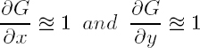
- – G is globally small, hence it is sufficient to match it only in the neighborhood of a pixel (equation [2.3]);
- – G is locally small, so its gradients are close to identities (equation [2.4]), justifying comparisons of windows of pixels instead of single pixels;
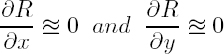
- – the gradient of R relative to p is small, hence it can be initially ignored (equation [2.5]).
Equations [2.3] and [2.4] may seem restrictive; however, in practice, it is sufficient that G is a smooth function and that we know an approximation ![]() of G (e.g. by assuming the mean altitude of the scene). When this is the case, we can compute a rectified image Ĩ2 of I2 that is defined by Ĩ2(p) = I2(
of G (e.g. by assuming the mean altitude of the scene). When this is the case, we can compute a rectified image Ĩ2 of I2 that is defined by Ĩ2(p) = I2(![]() (p)), and compute the image deformation ΔG between I1 and Ĩ2. Finally, we set the output deformation to G =
(p)), and compute the image deformation ΔG between I1 and Ĩ2. Finally, we set the output deformation to G = ![]() ° ΔG. This said, for the sake of simplicity, we assume in the following that equations [2.3] and [2.4] apply.
° ΔG. This said, for the sake of simplicity, we assume in the following that equations [2.3] and [2.4] apply.
2.2. Template matching
2.2.1. Matching as a similarity measure
Assuming that equation [2.3] is true, we can state that the correspondence of a pixel p is a pixel p′ = p + δ(p) with |δ(p)| < dmax, where dmax is a given threshold. When dmax is sufficiently small, thus avoiding ambiguity and long computation, the matching problem boils down to computing, for each pixel p, its most similar pixel in the search region given by D ∈ ‹−dmax, −dmax› (see Figure 2.1).
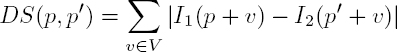
For a given pair I1, I2, let DS(p, p′) be the dissimilarity between two pixels p and p′ . If Nd is the neighborhood of size dmax, the matching algorithm is simply:
We now define a similarity measure that is both non-ambiguous and efficient to compute.
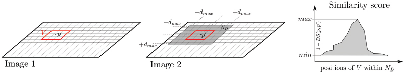
Figure 2.1. A toy example of the basic 2D template matching. A window V centered at p in Image 1 is moved in the search area ND of Image 2. At each position, a similarity score is computed for the pair of overlapping windows. The maximum score points to the best match of pixel p. For a color version of this figure, see www.iste.co.uk/cavalie/images.zip
2.2.2. Basic template approach
Ignoring the radiometric deformation R, let us have a closer look at equation [2.1]. Assuming hypothesis [2.4], we define a dissimilarity measure using the following formula, where V is the neighborhood that defines a window:
Note that the formula of equation [2.7] has a strong implication – it means that if p′ is the corresponding pixel of p, then for any v in the neighborhood V , p′ + v is the corresponding pixel of p + v. In other words, it is the hypothesis expressed in equation [2.4]; however, it is given in a discrete form. Of course, the key issue here is the size of the neighborhood V : if V is too small, then matching will be ambiguous; if V is too big, the above discrete hypothesis will not be true.
2.2.3. Normalized template approach
Let us now consider equation [2.2]. Due to radiometric deformation, for a pair of corresponding pixels p and p′ , I1(p) ![]() I2(p′) no longer holds true. Therefore, the formula from equation [2.7] cannot be used. The general guideline to handle this inconsistency is as follows:
I2(p′) no longer holds true. Therefore, the formula from equation [2.7] cannot be used. The general guideline to handle this inconsistency is as follows:
- – using equation [2.5], assume that, in a local neighborhood, the radiometric deformations do not depend on p; consequently, we have R(p, I2) = R(I2);
- – select a parametric model for R;
- – when testing the hypothesis that p is the correspondence of p′ , use all pairs of radiometries (I1(p + v), I2(p′ + v), v ∈ V ) to estimate the parametric model of R.
2.2.3.1. Rank normalization
Rank normalization is one of the most general parametric models, as it only imposes that R be a growing function. In the continuous case, i.e. with an infinite number of measurements, the normalization consists of histogram normalization. In the discrete case, as in the matching of a window of a finite size, this comes down to a rank normalization. That is, for each image Ik, and each pixel q in the neighborhood of p, compute the number of pixels with a value lower than q in the neighborhood V :
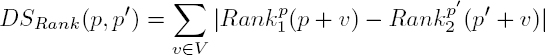
One of the drawbacks of this normalization is that it is relatively slow to compute. If N is the cardinal of V , a naive implementation can lead to a cost of N2 complexity. Using a quick sort algorithm to globally sort all values in V (p), the computation complexity can be reduced to N log(N).
2.2.3.2. Normalized cross-correlation
Most often, rank normalization is too general; therefore, more restrictive similarity measures are sought. A common model presumes that the radiometric deformation between I1 and I2 can be represented locally by an affine transform, with a being the translation and b the scaling factor:
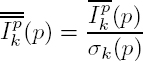
Using this assumption, we can compute normalized images ![]() independent of any affine transform within the window. This can be done in two steps:
independent of any affine transform within the window. This can be done in two steps:
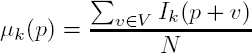
1) render the radiometry invariant to translation by subtracting the average of the radiometries (equation [2.11]);
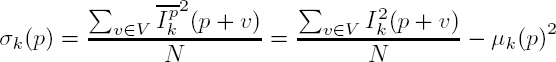
2) render the radiometry invariant to scaling by dividing it by its standard deviation (equation [2.12]).
where N is the number of pixels in the template (i.e. N = (2n + 1)2 for a square window of size n). For instance, in Figure 2.1, n = 1 and N = 9.
The average and standard deviations are computed from:
Immediately we can see that ![]() is invariant to any translation scaling in the radiometry:
is invariant to any translation scaling in the radiometry:
The normalized cross-correlation is then defined as a dissimilarity measure DS:
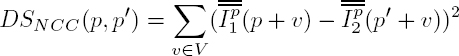
Alternatively, and as is often encountered in the literature, it is known as:
The above two expressions are closely related by:
The DSNCC dissimilarity measure remains the most popular similarity. Its wide use is due to numerous advantages:
- – it can be easily interpreted as a distance between normalized images;
- – the radiometric normalization to translation and scaling is justified by physical phenomena (e.g. changing illumination conditions);
- – DSNCC is always in the interval of [0 − 4], whereas NCC is always in the interval of [−1, 1]. They can be interpreted as distance and dot products between unit vectors (see equation [2.12]), which facilitates their interpretation or the fixing of certain parameters (e.g. thresholds, regularization parameters, etc.);
- – they are fast to compute. For instance, using the integral images, the computation time can be made to be independent of the size of the window.
2.2.3.3. Census coefficient
Rank distance and normalized cross-correlation use all the elements of the window to normalize the radiometry. As a result, in the presence of outliers, the normalization will be contaminated by false measurements. Outliers are not rare in image matching; for instance, when performing image matching for 3D geometry computation, outliers can arise systematically due to, for example, occlusions.
Census is a similarity measure that is robust to outliers and thus addresses the above shortcoming. To introduce census, let us define a binary operator ![]()
The operator applied to a window, ![]() converts it to a binary vector, where all elements larger than the value of the central pixel Ik(p) are true. By comparing such binary vectors computed for a pair of windows (centered at p and p′ in images I1 and I2, respectively), we obtain the census coefficient:
converts it to a binary vector, where all elements larger than the value of the central pixel Ik(p) are true. By comparing such binary vectors computed for a pair of windows (centered at p and p′ in images I1 and I2, respectively), we obtain the census coefficient:
What makes census robust is that the normalization is undertaken using only the value of the central pixel. Consequently, in the sum in equation [2.20], if there is an outlier, it will not influence the output score. Conversely, because of the strict normalization, the census coefficient is not very discriminant. With this in mind, we should apply census: (i) with large window sizes in order to bring “more” information or context into the measurement vector; or (ii) in combination with the regularization techniques described in section 2.3. A use case where census performs well is the computation of 3D scene geometry with severe occlusions.
2.2.3.4. Other similarity measures
There are many similarity measures and listing them all is beyond the scope of this chapter. Here, we mention several common alternatives:
- – Non-centered normalization: the only difference with the measure described in section 2.2.3.2 is that the average is not subtracted; as a result, it is less discriminant, as well as less sensitive to noise in textureless areas.
- – Mutual information (Viola and Wells 1997): this measure of similarity calculates the joint entropy between two random signals (e.g. two overlapping images). In general, the entropy is high if the information content is high (i.e. many variations of intensities in a textured region), and vice versa, the entropy is small for low information content (i.e. a flat region). For a pair of perfectly matched images, the joint entropy is low because one image predicts the content of the other, and therefore can be used as the matching cost. The similarity measure is particularly suitable to modeling important radiometric distortions; for example, image pairs acquired in different illumination conditions or even with sensors of different radiometric sensitivity.
- – Learning-based similarity measures (Žbontar and LeCun 2016): with the advances in machine learning and in particular deep learning, many state-of-the-art methods learn to predict the similarity of a pair of patches. The advantage of learning approaches is that they are able to learn an arbitrary function and hence model arbitrary geometric and radiometric deformations. On the downside, the parameters of the function are learnt by heart from specific training data and generalize poorly to other datasets.
2.3. Handling “large” deformations
2.3.1. Introduction
Limiting the matching problem to the definition of a similarity measure is possible when the search space is limited. When the search interval is increased, two limitations arise. First, the likelihood of erroneous matching grows with the growing number of tested hypotheses and leads to noisy results. Second, the computation time increases proportionally to the number of tested hypotheses.
In this section, we describe the most typical ways to solve the above-mentioned problems. The methods presented in section 2.3.2 address the robustness aspect, while in section 2.3.3, both the robustness and time issues are dealt with.
2.3.2. A posteriori filtering and regularization approach
As described in section 2.1.3, to solve the matching problem certain hypotheses about the regularity of the unknown geometric deformation G must be developed. However, by simply computing the most similar correspondence of a given pixel, there is no guarantee that the outcome deformation will comply with the regularity hypothesis. To impose it, the common practice is to force the geometric deformation to follow the hypothesis in equation [2.4].
A straightforward way to implement this behavior is to use an a posteriori filtering technique on the computed deformation values, for example:
- – a local mean filter – suitable for scenarios without outliers and when the expected deformation is a smooth function;
- – a local median filter – suitable for scenarios with outliers and when the expected deformation contains discontinuities;
- – a combination of the median and mean filters to eliminate the outliers and obtain a smooth deformation.
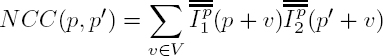
However, a posteriori filtering is only a post-processing technique and does not use all the available information to recover the “correct” deformation. Let us look at the scenario illustrated in Figure 2.2. Over a relatively large area, two alternative geometric deformations are presented as a blue line and a dashed line, respectively. The blue line is wrong, although it results from the most similar correspondences, and the dashed line is the real deformation but the second best result. In this scenario, filtering techniques are not capable of recovering the real deformation.
Figure 2.2. In the noisy data region, two geometric deformations are shown as a blue line and a dashed line resulting from the best and second best similarity scores, respectively. The second best result is the true deformation and can be recovered with regularization techniques. For a color version of this figure, see www.iste.co.uk/cavalie/images.zip
Ideally, we would like to guide the algorithm to perform the following: compute a deformation that maximizes the similarity measure but if there is a deformation with good enough similarity that is smoother (therefore more likely) than the first, choose the latter. In other words, the algorithm searches for a trade-off between similarity and regularity.
To formalize this, for a given deformation G, let us define the dissimilarity DS and the regularity Reg terms:
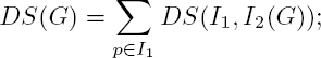
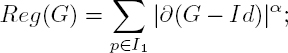
where the terms are defined over all pixels p of image I1, ∂(G − Id) is the gradient of G minus identity and α can take practically any value, but it should be chosen based on the characteristics of the deformation G (see Figure 2.3). Of course, the remarks at the end of section 2.1.3 also apply here, and Id can be replaced by any smooth a priori approximation of G.
Our aim is to find a solution that simultaneously minimizes DS and Reg. With the concepts presented up to now it is impossible, because the solution minimizing DS is the argument of the minimum for each pixel independently (defined in equation [2.6]), while the solution minimizing the regularity is simply the identity. An energetic approach allows us to handle this trade-off in a neat way by defining a function E:
Here, the deformation that we look for is defined as the deformation G that minimizes E. In equation [2.23], the term DS, known as the data term, depends only on the images, while Regα, known as the regularization, represents the a priori knowledge of the smoothness of G. The β factor allows us to control the relative importance of the data and regularization terms.
Currently, the energetic approach is the most common way to solve the matching problem, both in academic and commercial software solutions. It is an elegant and quite general way to combine the information brought by the data with the a priori information. When embarking on this approach, two non-trivial issues must be investigated: (1) the relation between the regularization term and the solution that will be favored; (2) once the function E is defined, the choice of the algorithm that can efficiently compute the deformation, minimizing equation [2.23]. An in-depth answer to these two questions is far beyond the scope of this chapter; however, in the following, we provide a brief commentary on the current methods.
Figure 2.3. The impact of the regularization term in equation [2.22] on the solution. The red lines represent the deformation G (displacement or the surface). In the dashed line zones, the image information is not discriminant enough to compute the deformation. The way the gap is filled with information depends on the value of the α parameter, which is represented by the blue, green and gray dashed lines. For a color version of this figure, see www.iste.co.uk/cavalie/images.zip
Regarding the impact of the regularization term, Figure 2.3 illustrates how α given in equation [2.22] can be used to favor diverse geometries. The dashed interval represents no image information and the red line corresponds to a region for which the image information is good enough to find the solution (i.e. deformation). Let us suppose that the solution in the information gap is steered only by the regularization term. Depending on the value of α, we can obtain different solutions:
- – α > 1: there is a unique solution, and it is the straight blue line that joins the red line on either end; this choice favors a smooth solution and is adequate for computing the 3D geometry of natural scenes without mountains;
- – α < 1: any path making the jump in a single step is the solution; this choice favors the solution with discontinuities and is adequate for computing the 3D geometry in urban areas;
- – α = 1: all the monotonous paths are the solutions; this is a neutral choice and adequate if the geometry is composed in the majority of smooth surfaces with some discontinuities, as in the case of coseismic deformations.
Concerning minimization algorithms, the most common methods are mincut–maxflow, semi-global matching (SGM) and variational methods. The mincut–maxflow computes the exact minimum of equation [2.23]; however, it imposes that α ≥ 1 and is relatively costly in time and space (i.e. it has high memory consumption). The SGM is a version of the dynamic programming method. It is not limited by the value of α and is efficient in both time and space. On the downside, it does not compute the exact minimum, which sometimes leads to unpleasant artifacts. Finally, the variational approach uses nonlinear least squares to solve equation [2.23]. As the deformation G is computed globally, there is no need to use the template method; as a result, the solution does not suffer from the artifacts specific to the window-based method. A drawback is that the variational approach requires good initialization of G.
2.3.3. Multi-resolution approach
When dealing with large deformations, the regularization approach partially solves the robustness issue but not the CPU issue. In fact, it increases the total computation time by having to include the regularization. Multi-resolution processing, a particular case of the “coarse to fine” strategy, can further improve the two aspects (Pierrot-Deseilligny and Paparoditis 2006; Rothermel et al. 2012). The strategy is to first obtain an approximate and fast (i.e. coarse) solution and then to use it to compute a finer solution. A basic multi-resolution approach can be described as follows:
- – compute down-sampled images at half the resolution:
- – compute the geometric deformation G between I1 and I2; note that the images have four times fewer pixels, and the research intervals are two or four times smaller (in 1D or 2D matching, respectively), hence the computation is theoretically 8–16 times faster;
- – use G as a predictor to limit the research interval in full-resolution images.
This procedure is typically used recursively by computing a pyramid of images and starting the computation with the lowest resolution images. For example, in MicMac software (Rosu et al. 2015), when processing large satellite images, the downsampling currently goes to 1/32 or 1/64 at the lowest resolution.
2.4. Discrete nature of the image and sub-pixel matching
Until now we have made the implicit assumption that for a given pixel p with integer coordinates, its corresponding pixel is also a pixel q with integer coordinates. The drawback of this assumption is that we can only compute integer deformations and this thus reduces the accuracy of the measurement. Sub-pixel deformations cannot be determined because they are invisible to the matching algorithm. Typically, if we work with satellite images of 10 m resolution, this “integer” approach would limit the accuracy to 5 m.
There are two ways to overcome this shortcoming, both based on interpolation, which we refer to as the interpolation of similarity and the similarity of interpolation. In the interpolation of similarity, for a given pixel, we (1) compute and memorize the similarity calculated in the search region, using integer pixels, (2) use some quadratic function to model the similarity function and finally (3) extract its maximum. In the similarity of interpolation, we select an interpolating algorithm and use it to extract the value of I2 using non-integer pixels (i.e. at sub-pixel positions). This approach is generally slower but more general. To limit the signal aliasing, precautions must be taken in selecting the interpolating kernel.
Using such techniques, it is possible to achieve the accuracy of ![]() of a pixel. Nevertheless, the accuracy remains largely dependent on the images (e.g. the sensor, the scene type, etc.) and may vary from
of a pixel. Nevertheless, the accuracy remains largely dependent on the images (e.g. the sensor, the scene type, etc.) and may vary from ![]() in an unfavorable condition to
in an unfavorable condition to ![]() 100 in very favorable conditions.
100 in very favorable conditions.
2.5. Optical imaging sensors
In the previous sections, we used an implicit assumption that in both forms of matching (1D and 2D), we could approximately predict the position of corresponding pixels. This prediction is possible thanks to the known geometry of the sensors with which the images are acquired. The geometries describe position and rotation in 3D space and enable relating images taken from different viewpoints.
2.5.1. Sensor geometries
The two common classes of sensor geometries are frame and pushbroom geometries. Frame cameras dispose of an area array sensor in which all the pixels share the same optical center and are exposed to light simultaneously1. Pushbroom cameras, in contrast, are composed of a linear sensor array and scan the scene along the trajectory of the sensor. As a result, each image line is acquired at a different time and from a unique position in space, following the perspective projection along the linescan and the orthogonal projection in the perpendicular direction. In fact, the real pushbroom sensors used in spaceborne imaging have a complex layout that is often composed of several detectors situated in the focal plane (Lier et al. 2008). To facilitate the use of the images, the images undergo resampling to create an ideal sensor. The ideal sensor simulates a single-line pushbroom sensor, free from optical distortions and from the jitter artifacts caused by high-frequency attitude changes (De Lussy et al. 2005).
Until recently, frame cameras were more common in terrestrial and airborne applications, whereas pushbroom scanners were a standard in spaceborne imaging. Thanks to technological advances and lower costs, we can observe more and more of the frame arrays used in satellites (e.g. Planet’s CubeSat constellations).
2.5.2. Sensor orientation in 3D space
2.5.2.1. Physical model
Sensor orientation in 3D space is carried out in two steps by applying the so-called intrinsic and extrinsic calibration parameters. The intrinsic parameters allow us to associate a pixel measurement in the 2D image coordinates with a bundle in 3D space. The extrinsic parameters orientate the camera in the world coordinate frame; in other words, they allow us to georeference a camera. These steps are realized by three consecutive operations: ![]() transformation from the world to the camera coordinates;
transformation from the world to the camera coordinates; ![]() perspective projection from 3D to 2D camera coordinates; and finally
perspective projection from 3D to 2D camera coordinates; and finally ![]() from a 2D camera to image coordinates. This mapping can be represented in a compact equation form, referred to as the collinearity equation (see Figure 2.4):
from a 2D camera to image coordinates. This mapping can be represented in a compact equation form, referred to as the collinearity equation (see Figure 2.4):
where Rk and Ck are the extrinsic orientation parameters of some image k; in particular, Rk is the rotation matrix that moves from world coordinates to camera coordinates, and Ck is the image perspective center in the world coordinates; ![]() represents the perspective projection; I indicates the intrinsic parameters (i.e. the focal length, the principal point and the distortions) and pk the image coordinates (i, j)k of the point P in some image k.
represents the perspective projection; I indicates the intrinsic parameters (i.e. the focal length, the principal point and the distortions) and pk the image coordinates (i, j)k of the point P in some image k.
Equation [2.24] holds true for frame cameras, i.e. when all pixels are exposed at the same instant. To take into account pushbroom cameras, we should generalize the above equation by including the time component t:
The projection equation of this form is rigorous because it describes the passage from the 3D ground scene to the 2D image space using physical parameters. The physical nature of the parameters is considered advantageous because they (i) are seldom correlated, (ii) can be easily interpreted, and (iii) can be optimally adjusted. Nonetheless, for several reasons, the rigorous model is rarely used in practice. One of its main drawbacks is the lack of standardization among the satellite image providers, hence the difficulty in maintaining those models in various software solutions. Another drawback is due to its complexity and, in particular, the fact that the number of unknowns grows with the number of image lines. In response to this, several sensor replacement models have been proposed over the last 40 years. Among them are the polynomial image geometry model; the grid interpolation model; the rational function model (RFM), also known as the rational polynomial coefficient (RPC) model; and the replacement sensor model (RSM). Nowadays, the RPC model is the prevalent choice to describe the geolocation of a satellite sensor; therefore, we discuss it further in the next section.
Note that equation [2.25] does not explicate the ray’s refraction effects but assumes rays to be straight lines. In practice, image rays are bent as they pass through the different layers of the atmosphere, and to compensate for this phenomena, image corrections are applied. The atmospheric refraction correction is inversely proportional to the square of the focal length; therefore, it is less pronounced for narrow-angle satellite sensors. For example, for near-vertical acquisitions by Pleiades satellites with an incidence angle of 15°, the geolocalization error reaches approximately 2 m (see the Pléiades Imagery User Guide). For more details on sensor models, see OpenGIS Consortium (1999) and McGlone (2013).
2.5.2.2. Empirical model – rational polynomial coefficients
The RPC model relates the ground coordinates and the image coordinate using two rational polynomial functions:
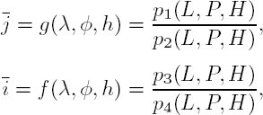
where ![]() are the normalized sample (column) and line (row) indices; (λ, φ) are the latitude and longitude coordinates in the WGS-84 geodetic system and (L, P) are their normalized equivalents; h and H are the ellipsoidal altitude and its normalized equivalent, respectively; and pi indicates polynomials of the third order; the normalization is defined in the range
are the normalized sample (column) and line (row) indices; (λ, φ) are the latitude and longitude coordinates in the WGS-84 geodetic system and (L, P) are their normalized equivalents; h and H are the ellipsoidal altitude and its normalized equivalent, respectively; and pi indicates polynomials of the third order; the normalization is defined in the range ![]()
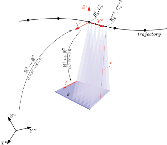
Figure 2.4. Sensor orientation in 3D space. (X, Y, Z)w and (X, Y, Z)c are the respective world and camera frames.  are the extrinsic parameters of some image k at time t, (i, j) are the image coordinates and f is the focal length. For a color version of this figure, see www.iste.co.uk/cavalie/images.zip
The accuracy of the RPC model is conditioned by the estimation method. We can distinguish between terrain-dependent (from ground control points (GCPs)) and terrain-independent (from the physical sensor model) estimation methods. If the RPCs are generated from the physical sensor model, the accuracy is generally as good as that of the model that served to estimate the coefficients. If the physical sensor is not available (e.g. due to poor performance of the on-satellite direct measurement devices), the quality of the RPCs is highly dependent on the number as well as the distribution of GCPs and deteriorates quickly with insufficient number points (Tao and Hu 2001b). It should be noted that the rational polynomial functions are generally not capable of modeling high-frequency distortions caused, for example, by a satellite’s vibrations. We owe their accuracy to the image pre-processing step that transforms the real sensor to an ideal one (De Lussy et al. 2005).
Even though RPC-encoded geolocation is precise with regard to the physical model, the accuracy – i.e. the absolute precision with respect to some Earth-fixed coordinate frame – is not guaranteed. The RPCs delivered customarily with Pléiades, SPOT-6/7, QuickBird, WorldView, PlanetScope, GeoEye, Ikonos, Cartosat, etc., can be misaligned by up to 10 pix (CE90), equivalent to several meters on the ground (Oh and Lee 2015). Such deviations are due to errors in direct measurements on board the satellite (i.e. GNSS, gyros, star trackers), especially errors in attitude and position (Fraser and Hanley 2005). These may hinder further processing; for example, the digital surface model generation with matching algorithms (d’Angelo 2013). Note that due to the short-term correlation of onboard measurements, errors in RPC geolocation from in-orbit acquisitions are less pronounced than errors from multi-orbit and multi-epoch acquisitions. The RPC model is therefore usually subject to refinement. For narrow field-of-view sensors, as in the satellite pushbroom camera, the attitude errors induce the same net effect on the ground as do the in- and across-track positioning errors. As a result of this correlation, sensor errors can be modeled with two correction functions that are defined in the image coordinates: (1) δf in the line direction, to absorb the in-track orbit and pitch errors; and (2) δg in the sample direction, to absorb the equivalent across-track errors (Grodecki and Dial 2003):
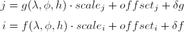
where δg and δf are polynomials. The parameters of the correction functions are estimated in a least squares adjustment with image correspondences and GCPs used as observations. To strengthen the solution, the equations can include additional constraints imposing that the (δg, δf) displacement fields follow a global sensor rotation (Rupnik et al. 2016). The GCPs are commonly collected using existing databases of orthophoto images and global digital elevation models; for instance, the Sentinel-2 and Shuttle Radar Topography Mission (SRTM) DEMs (Kääb et al. 2017).
2.5.2.3. Epipolar model
Given a pair of overlapping images and their known geometries, in order to predict positions of their corresponding points, we often resort to the so-called epipolar geometry. Epipolar geometry is mainly useful in two tasks: relative orientation of an image and image matching for digital surface model (DSM) generation. During the relative orientation of frame cameras, the epipolar constraint is written into the essential matrix from which the rotation and translation of two images can be decomposed. DSM computation reduces the correspondence search from a 2D problem (i.e. a pixel in one image matched against every pixel in the other image) to a line or a curve of candidates.
To illustrate the epipolar geometry of the original image pair, let us look at Figure 2.5. By applying the intrinsic and extrinsic parameters in equations [2.24]–[2.25] to some pixel p in image I1, we obtain a 3D bundle Bp associated with that position. This bundle, projected to an overlapping image I2 via a plane π anchored at the projection centers O1 and O2, will intersect the focal plane of the image I2, giving rise to the epipolar line ep (see Figure 2.5). In other words, for some pixel p, the above relationship predicts the position of its candidate corresponding points in another image.
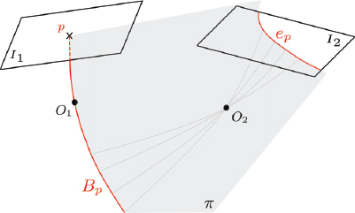
Figure 2.5. Epipolar line ep as a projection of a bundle Bp via the epipolar plane π. For a color version of this figure, see www.iste.co.uk/cavalie/images.zip
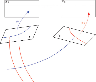
Figure 2.6. An image pair in the original geometry (bottom) and rectified to the epipolar geometry with functions φ1, φ2 (top). For a color version of this figure, see www.iste.co.uk/cavalie/images.zip
In image matching, it is useful to separate the correspondence search from orientation parameters. To undertake this, an image pair can be rectified to an equivalent geometry, so that the corresponding epipolar lines are aligned and parallel to image rows (see Figure 2.6). From then on, the image matching comes down to finding conjugate points across lines with the same y-coordinate, with no regard to the image geometry. For frame cameras, the rectification to the equivalent geometry involves applying two 2D projective transformations to both images of a stereo pair. Unlike the frame cameras, pushbroom sensors acquire each image row from a different perspective center, and as a result, the epipolar lines are neither straight lines nor are they conjugate across the image (Gupta and Hartley 1997). State-of-the-art approaches leverage this by either rectifying the image per patch, assuming that locally the epipolar curves are straight lines (de Franchis et al. 2014), or mapping the epipolar curves across the images, followed by a rectification transformation that straightens the curves to lines (Oh 2011; Pierrot-Deseilligny and Rupnik 2020).
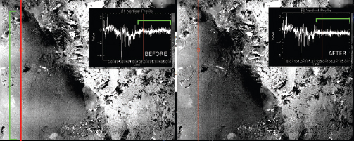
Figure 2.7. The effect of unmodeled sensor errors on image matching. The left image corresponds to a displacement map before correction and the right image corresponds to a displacement map after correction (Delorme et al. 2020). For a color version of this figure, see www.iste.co.uk/cavalie/images.zip
2.5.2.4. Unmodeled sensor errors
Independent of the orientation model, refined sensor parameters still reveal errors related to the unmodeled satellite’s attitude and the CCD chip’s misalignment (Ayoub et al. 2008). In Figure 2.7 we can observe the effect such discrepancies have on image matching. The left image shows a displacement map obtained from matching of two ortho-rectified images. The lower left part of the image is corrupted with an oscillating signal along the vertical axis, caused by the satellite’s jitter. The induced artifacts can be up to several pixels and, therefore, for high accuracy measurements, must be eliminated. A common technique consists of modeling and subtracting the undulating signal in post-processing (Delorme et al. 2020; Michel et al. 2020).
2.6. Acknowledgments
We thank Renaud Binet and Amaury Dehecq for their careful reviews and comments that helped to improve this chapter.
2.7. References
d’Angelo, P. (2013). Automatic orientation of large multitemporal satellite image blocks. Proceedings of the International Symposium on Satellite Mapping Technology and Application, 1–6.
Ayoub, F., Leprince, S., Binet, R., Lewis, K.W., Aharonson, O., Avouac, J.-P. (2008). Influence of camera distortions on satellite image registration and change detection applications. IEEE International Geoscience and Remote Sensing Symposium, Boston, USA, 6–11 July.
De Lussy, F., Kubik, P., Greslou, D., Pascal, V., Gigord, P., Cantou, J.P. (2005). Pleiades–HR image system products and geometric accuracy. Proceedings of the International Society for Photogrammetry and Remote Sensing Workshop, Hannover, Germany.
Delorme, A., Grandin, R., Klinger, Y., Pierrot-Deseilligny, M., Feuillet, N., Jacques, E., Rupnik, E., Morishita, Y. (2020). Complex deformation at shallow depth during the 30 October 2016 Mw 6.5 Norcia earthquake: Interference between tectonic and gravity processes? Tectonics, 39(2), e2019TC005596.
de Franchis, C., Meinhardt-Llopis, E., Michel, J., Morel, J.-M., Facciolo, G. (2014). On stereo-rectification of pushbroom images. IEEE International Conference on Image Processing (ICIP), Paris, France, 27–30 October.
Fraser, C.S. and Hanley, H.B. (2005). Bias-compensated RPCS for sensor orientation of high-resolution satellite imagery. Photogrammetric Engineering and Remote Sensing, 71(8), 909–915.
Grodecki, J. and Dial, G. (2003). Block adjustment of high-resolution satellite images described by rational polynomials. Photogrammetric Engineering and Remote Sensing, 69(1), 59–68.
Gupta, R. and Hartley, R.I. (1997). Linear pushbroom cameras. IEEE Transactions on Pattern Analysis and Machine Intelligence, 19(9), 963–975.
Horn, B.K. and Schunck, B.G. (1981). Determining optical flow. Artificial Intelligence, 17(1–3), 185–203.
Kääb, A., Altena, B., Mascaro, J. (2017). Coseismic displacements of the 14 November 2016 Mw 7.8 Kaikoura, New Zealand, earthquake using the Planet optical Cubesat constellation. Natural Hazards and Earth System Sciences, 17, 627–639.
Leprince, S., Barbot, S., Ayoub, F., Avouac, J.-P. (2007). Automatic and precise orthorectification, coregistration, and subpixel correlation of satellite images, application to ground deformation measurements. IEEE Transactions on Geoscience and Remote Sensing, 45(6), 1529–1558.
Lier, P., Valorge, C., Briottet, X. (2008). Imagerie spatiale : des principes d’acquisition au traitement des images optiques pour l’observation de la terre. Editions Cépadues, Toulouse, France.
Lowe, D.G. (2004). Distinctive image features from scale-invariant keypoints. International Journal of Computer Vision, 60(2), 91–110.
Madden, F. (1999). The Corona camera system – Iteks contribution to world security. JBIS, 52, 379–396.
McGlone, C. (ed.) (2013). Manual of Photogrammetry. American Society of Photogrammetry and Remote Sensing, Bethesda, MD, USA.
Michel, J., Sarrazin, E., Youssefi, D., Cournet, M., Buffe, F., Delvit, J., Emilien, A., Bosman, J., Melet, O., L’Helguen, C. (2020). A new satellite imagery stereo pipeline designed for scalability, robustness and performance. ISPRS Annals of the Photogrammetry, Remote Sensing and Spatial Information Sciences, 2, 171–178.
Oh, J. (2011). Novel approach to epipolar resampling of HRSI and satellite stereo imagery-based georeferencing of aerial images. PhD thesis, Ohio State University, Ohio, USA.
Oh, J. and Lee, C. (2015). Automated bias-compensation of rational polynomial coefficients of high resolution satellite imagery based on topographic maps. ISPRS Journal of Photogrammetry and Remote Sensing, 100, 14–22.
OpenGIS Consortium (1999). The openGIS Abstract Specification – Topic 7: Earth Imagery Case.
Pierrot-Deseilligny, M. and Paparoditis, N. (2006). A multiresolution and optimization-based image matching approach: An application to surface reconstruction from SPOT5-HRS stereo imagery. ISPRS Workshop on Topographic Mapping from Space, Ankara, Turkey.
Pierrot-Deseilligny, M. and Rupnik, E. (2020). Epipolar rectification of a generic camera. Preprint [Online]. Available at: https://hal.archives-ouvertes.fr/hal-02968078.
Rosu, A., Pierrot-Deseilligny, M., Delorme, A., Binet, R., Klinger, Y. (2015). Measurement of ground displacement from optical satellite image correlation using the free open-source software MicMac. ISPRS Journal of Photogrammetry and Remote Sensing, 100, 48–59.
Rothermel, M., Wenzel, K., Fritsch, D., Haala, N. (2012). Sure: Photogrammetric surface reconstruction from imagery. LC3D Workshop, Berlin, Germany.
Rupnik, E., Deseilligny, M.P., Delorme, A., Klinger, Y. (2016). Refined satellite image orientation in the free open-source photogrammetric tools Apero/MicMac. ISPRS Annals of the Photogrammetry, Remote Sensing and Spatial Information Sciences, 3, 83.
Tao, C.V. and Hu, Y. (2001a). A comprehensive study of the rational function model for photogrammetric processing. Photogrammetric Engineering and Remote Sensing, 67(12), 1347–1358.
Tao, C.V. and Hu, Y. (2001b). Use of the rational function model for image rectification. Canadian Journal of Remote Sensing, 27(6), 593–602.
Viola, P. and Wells, W.M. (1997). Alignment by maximization of mutual information. International Journal of Computer Vision, 24(2), 137–154.
Žbontar, J. and LeCun, Y. (2016). Stereo matching by training a convolutional neural network to compare image patches. The Journal of Machine Learning Research, 17(1), 2287–2318.
- 1. With the exception of frame sensors that use rolling shutters and scan the image line by line, thus violating this assumption.