
12
New Applications of Spaceborne Optical Image Cross-Correlation: Digital Elevation Models of Volcanic Clouds and Shallow Bathymetry from Space
Marcello DE MICHELE and Daniel RAUCOULES
BRGM, Orléans, France
12.1. Introduction
12.1.1. General introduction
In this chapter, we describe how we create offset maps by using cross-correlation between two satellite images in an unconventional way. Instead of using images acquired at multiples dates, as we do in SAR/optical offset tracking or SAR interferometry, we use two images from the same acquisition date and from the same dataset. The reader needs to know that within the pushbroom sensor geometry, the physical separation of panchromatic and multispectral charge-coupled device (CCD) bands on the focal plane of the instrument yields a baseline and a temporal lag between the two images. The baseline is associated with a base-to-height (B/H) ratio that is sufficient to extract the elevation models of a tall object such as a volcanic ash cloud. The time lag also yields pixel offsets. These offsets, perpendicular to the epipolar direction, are proportional to the ash cloud velocity or, if the dataset is acquired over the sea, to the wave celerity. In the following section, we concentrate on how this physical separation and time lag can be used as an instrument itself. We will see how we can exploit it to create a digital elevation model of the volcanic ash cloud. Moreover, we will see how we can measure wave celerity from space and how this parameter is related to water depth, that is, bathymetry.
12.2. Digital elevation models of volcanic ash clouds
12.2.1. Introduction: can we precisely measure the height of a volcanic ash cloud and what physical process controls the injection height and the speed of a volcanic ash plume?
The routine retrieval of both the height and velocity of volcanic clouds is a crucial point in volcanology. The injection altitude is an important parameter that controls the ash and gas dispersion in the atmosphere and their impact and lifetime around the Earth. As is known today, information on the volcanic cloud height is critical for ash dispersion modeling and air traffic security. The volcanic cloud height related to explosive volcanism is indeed the primary parameter for estimating the mass eruption rate. A number of other reasons also make the volcanic cloud altitude a key parameter to measure: for example, the retrieval of the SO2 concentration from dedicated spaceborne spectrometers (Corradini et al. 2009) and the distribution of ash deposits on the ground during a given eruption. Furthermore, the understanding of a large part of the volcanic system itself strongly relies on knowledge of the volcanic cloud height since the physical characteristics of the cloud are related to key parameters of the volcanic system beneath the surface. For example, the ash and gas emission rates are related to the state of pressurization of the magmatic chamber at depth. The height reached by a volcanic cloud, together with the atmospheric wind regime, controls the dispersal of tephra, the fragmental material of any size and composition produced by a volcanic eruption. The eruption column is itself a function of quite a few important physical parameters, such as the vent radius, gas exit velocity, gas content of eruption products and efficiency of conversion of thermal energy contained in juvenile material to potential and kinetic energy during the entrainment of atmospheric air (Wilson et al. 1978). Conventional photogrammetric restitution based on satellite stereo imagery cannot precisely retrieve a spatially detailed digital elevation model of volcanic plumes or plume elevation models (PEMs), as the plume’s own velocity – mostly due to the wind – induces an apparent parallax that adds up to the standard parallax given by the stereoscopic view. Therefore, measurements based on standard satellite photogrammetric restitution do not apply here, as there is an ambiguity in the measurement of the plume position. Other methods exist, which we do not treat in detail here but we wish to mention for the curious reader. The earliest use of satellite data to estimate ash cloud heights with photogrammetric methods relied on manually measuring the length of the shadow cast by the cloud under known illumination conditions (Prata and Grant 2001; Spinetti et al. 2013). This technique is still used today (Pailot et al. 2020). In the literature, we can find some approaches to cloud photogrammetry using instruments with multi-angle observation capabilities; for example, Prata and Turner (1997) used the forward and nadir views of the along-track scanning radiometer (ATSR) to determine volcanic cloud top height (VCTH) for the 1996 Mt. Ruapehu eruption. The multi-angle imaging spectroradiometer (MISR) has been used to retrieve the VCTH, optical depth, type and shape of the finest particles for several eruptions (Scollo et al. 2010; Nelson et al. 2013; Flower and Kahn 2017).
12.2.2. Principles
The method that we describe here is a geometric technique. Consequently, height estimates are not sensitive at all to radiometric calibration uncertainties or to the emissivity of the plume material. In this method, we use optical sensors with a very high spatial resolution in the range of 30–10 m (e.g. Landsat 8, Sentinel 2) and 0.5 m (e.g. Pléiades). This method only works with non-transparent volcanic plumes. It restitutes high-resolution maps of volcanic cloud top height and horizontal velocities, as described by de Michele et al. (2016).
The general concept for extracting a plume elevation model is that the panchromatic (PAN) and the multispectral (MS) sensors onboard a pushbroom satellite platform cannot occupy the same position in the focal plane of the instrument (Figure 12.1). Therefore, there is a physical separation between the two CCDs. This geometry is key and relies on the concept of the sensor itself. We remind the reader that this sensor was not built on purpose to extract PEMs; we actually exploit a default of the sensor geometry to prove a concept. This CCD separation yields a baseline and a time lag between the PAN and MS image acquisitions. On the one hand, the small baseline has already been successfully exploited for retrieving digital elevation models (DEMs) of still surfaces such as topography or building heights (e.g. Massonnet et al. 1997; Vadon 2003; Mai and Latry 2009). On the other hand, the time lag has been successfully exploited to measure the velocity field of moving surfaces, such as ocean waves and arctic river discharges (de Michele et al. 2012; Kääb and Leprince 2014).
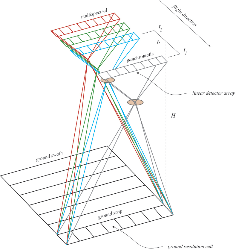
Figure 12.1. Simplified geometry of the focal plane of a pushbroom sensor. This illustration stretches out the separation between the panchromatic CCD and the multispectral CCDs. This separation yields a time lag (t1 and t2) as well as a baseline (distance b). These two values can be used to measure the heights and velocities of features in the scenes. Illustration by M. de Michele, ©BRGM. For a color version of this figure, see www.iste.co.uk/cavalie/images.zip
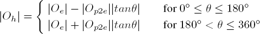
We consider two main directions: the epipolar (EP) direction, i.e. the azimuth direction of the satellite (i.e. the flight direction), and the perpendicular to the EP (P2E) direction. The pixel offset between PAN and MS sensors in the EP direction is proportional to the height of the plume plus the pixel offset contribution induced by the motion of the plume itself in between the two acquisitions. The pixel offset in the P2E direction, also controlled by the time lag, is proportional to the plume motion only, as there is no parallax in the P2E direction by definition. In principle, the offset in the P2E direction is proportional to the movements of every feature in the imaged scene (e.g. meteorological clouds, lahars, river flow, ocean waves, vehicles). In our case study, we are only interested in the volcanic cloud motion. We use this latter information to measure the volcanic cloud velocity and to compensate for the apparent parallax recorded in the EP offset. Sometimes things become complicated because the focal plane of the instrument is not made of long CCDs, as in the Centre National d’Etudes Spatiales (CNES) SPOT family, but of small focal plane modules (FPMs), such as the National Aeronautics and Space Administration/United States Geological Survey (NASA/USGS) Landsat 8 or the European Union/ESA (European Space Agency) Copernicus program Sentinel 2 satellite. For instance, the Landsat 8 operational land imager (OLI) instrument is a pushbroom (linear array) imaging system that collects visible, near infra-red and short-wave infra-red spectral band imagery at 30 m multispectral and 15 m panchromatic ground sample distances. It collects 190 km wide image swaths from 705 km orbital altitude. The OLI detectors are distributed across 14 separate FPMs, each of which covers a portion of the 15° OLI cross-track field of view. The internal layout of all the 14 FPMs is the same for all the FPMs, with alternate FPMs being rotated by 180° to keep the active detector areas as close together as possible. This feature has the effect of inverting the along-track order of the spectral bands in adjacent FPMs. Consequently, this has the effect of inverting the signs of the cross-correlation measurements when calculating pixel offsets between PAN and MS bands, which is related to the volcanic cloud velocity and parallax. The Copernicus Sentinel 2 focal plane hosts a similar geometry, called a “staggered” geometry. A correlator is used to perform pixel (or sub-pixel) offset measurements. If we consider the OLI image as a matrix made of lines and columns, offsets among the lines are the EP offsets Oe, while offsets among columns are the P2E offsets (Op2e). In the offset map, there may exist a ramp resulting from band misregistration; the ramp, if found, is removed. The direction of the plume (θ) is measured with respect to the azimuth direction, with the convention depicted in Figure 12.2. The absolute value of the pixel offsets due to the VCTH is calculated as Oh. We have to take into account that Oe has the same sign throughout the image. However, the wind direction does not. If we make the assumption that the plume direction is driven by the wind, there are cases where |Op2e||tanθ| has to be subtracted and there are cases where it has to be added to Oe, depending on whether the wind-generated offset is the same sign with respect to Oe or not. In the first case, the wind generates an apparent parallax that adds up to the one generated by the plume height; therefore, |Op2e||tanθ| needs to be subtracted. In the latter case, the wind generates an apparent parallax that subtracts from the one generated by the plume height; therefore, |Op2e||tanθ| needs to be added (Figure 12.2). To sum up, generally, Oh from staggered sensors should be calculated as follows:
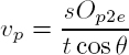
For each pixel, Oh is then converted into a VCTH using the formula:
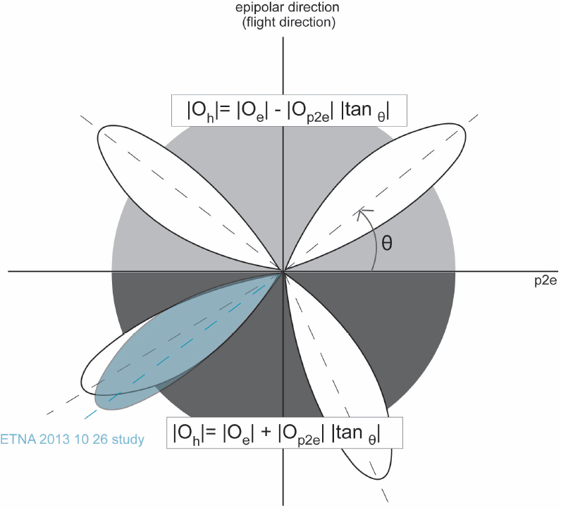
Figure 12.2. Conventions for RAW images when the spacecraft is flying positive along the Y axis: a simplified illustration of plume directions, θ, the epipolar direction, the P2E direction and the formulas to use if the plume is in the top or bottom quadrants. The plume is represented by the white lobe, with an example from Etna, October 26, 2016 (blue lobe). For a color version of this figure, see www.iste.co.uk/cavalie/images.zip
The result is a digital elevation model of the volcanic ash cloud. Here, h is the plume height (m), s is the pixel size (m), V is the platform velocity (m/s), t is the temporal lag between the two image bands (s) and H is the platform height (m). Peculiar cases are: θ = 15° and θ = 180°. In these cases, the system is no longer sensitive to the plume velocity. Therefore,
If θ = 90° and θ = 270°, the methodology is no longer applicable as the plume velocity yields an apparent parallax that is non-separable from the height-related parallax. In addition to the height of the ash cloud, this method provides a spatially dense measure of the ash cloud velocity at the PEM pixel resolution:
12.2.3. Applications
The extraction of digital elevation models of volcanic ash plumes, and their velocities, from pushbroom sensors is based on a rather new methodology. Therefore, examples are limited to only a few published studies (de Michele et al. 2016, 2019). In the following sections, we present some examples found in the literature using sensors from the Landsat 8 mission and the Pléiades mission.
12.2.3.1. Holuhraun (Landsat 8)
The 2014–2015 Holuhraun eruption in the Bárðarbunga volcanic system was the largest fissure eruption in Iceland since the 1783 Laki eruption. It started at the end of August 2014 and lasted six months, until late February 2015. It was characterized by large degassing processes and emission of SO2 into the atmosphere. The eruption steam and gas column were nicely captured by Landsat 8 on September 6, 2014 at 12:25 UTC (Figure 12.3). The nominal PAN/red time lag for Landsat 8 is 0.52 seconds, while the nominal angular separation is 0.3 degrees. The platform flies at a nominal altitude of 705 km and a nominal speed of 7.5 km/s. Therefore, the base-to-height ratio (b/h) is 0.0055. Alternatively, we can use the green channel instead of the red (the time lag of which is 0.65 s), or both. We chose the Holuhraun eruption as it represents a challenging test case for us, as its plume was rapidly moving and reached low altitudes. Therefore, if our method works on the Holuhraun test case, then it should apply to other types of volcanic plumes (higher and slower).
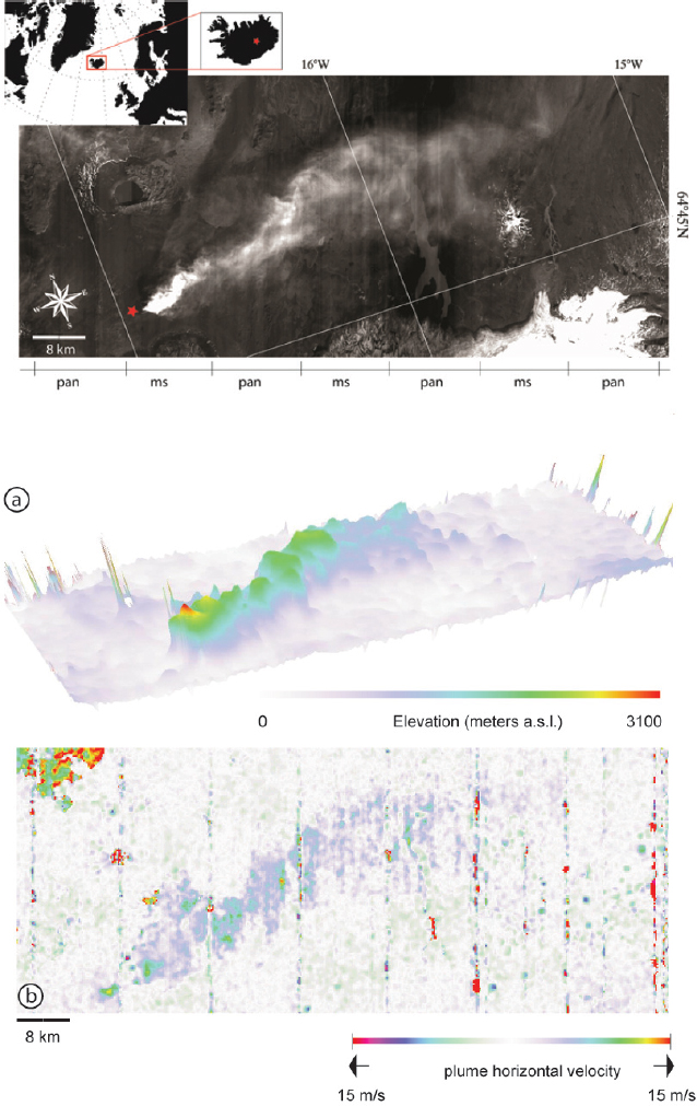
Figure 12.3. Top: the Holuhraun eruption seen in the reconstructed image from Landsat, which is made up of alternating panchromatic (pan) and multispectral (ms) bands. (a) The digital elevation model of the volcanic cloud, visualized in 3D, was obtained by applying the proposed method. (b) A map of the resulting horizontal velocities associated with the volcanic cloud. For a color version of this figure, see www.iste.co.uk/cavalie/images.zip
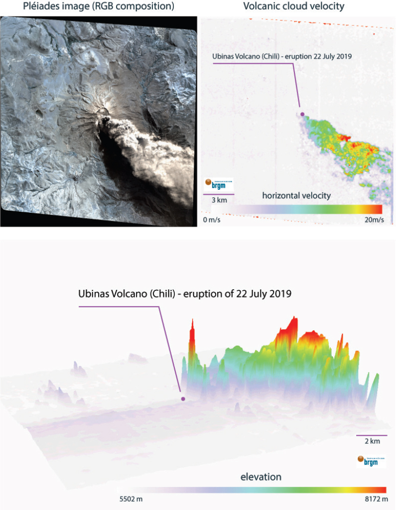
Figure 12.4. Top left: Ubinas volcano eruption as seen from the Pléiades satellite. Top right: the horizontal velocity of the volcanic cloud measured from the cross-correlation of Pléiades images. Bottom: a 3D visualization of the volcanic plume elevation model extracted from Pléiades images. Courtesy of BRGM; Pléiades data provided by CNES; processing done in the framework of the French CIEST2 initiative. For a color version of this figure, see www.iste.co.uk/cavalie/images.zip
12.2.3.2. Ubinas 2019 (Pléiades)
Ubinas is Peru’s most active volcano. It is the northernmost of three young volcanoes located along a regional structural lineament east of the main volcanic front of Peru. It has had 10 eruptions since 1900, with the last being reported in November 2016. On July 19, 2019, the Ubinas volcano started to erupt (Figure 12.4). An ash plume developed and the ashes fell on several departments of southern Peru. The International Charter “Space and Major Disasters” was activated following Peru declaring a state of emergency for the areas surrounding the Ubinas volcano. Via the International Charter “Space and Major Disasters”, the CNES programmed several acquisitions from the Pléiades satellite, the very high resolution panchromatic and multispectral imager. A clear image was acquired on July 19th, with an ash plume clearly visible in the dataset. We used the lag between the panchromatic and the multispectral CCDs in the Pléiades data to extract a digital elevation model of the volcanic ash plume and a map of the plume horizontal velocity. This information, along with ash plume roughness, is crucial for atmospheric physicists to update ash dispersion models. In this exercise, we proved the concept and tested the potential of Pléiades data for ash plume height monitoring.
12.2.3.3. Etna (SPOT-1)
The methodology can be applied to past volcanic eruptions, which opens the way to the investigation of ash cloud injection heights in the past. Mount Etna is one of the most active volcanoes in Europe. The years 2001 and 2002 were marked by intense episodes of flank eruptions. These eruptions generated a large ash clouds. The SPOT-2 satellite captured the eruption on July 27, 2001, which was used in this exercise to retrieve a digital elevation model of this particular ash cloud (Figure 12.5).
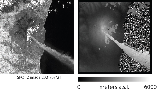
Figure 12.5. Left: Etna flank eruption as seen by SPOT-2 on July 21, 2001. Right: the volcanic cloud digital elevation model extracted from SPOT-2. For a color version of this figure, see www.iste.co.uk/cavalie/images.zip
12.3. Shallow bathymetry: measuring wave characteristics from space
12.3.1. Introduction: can we map tectonic fault motion under shallow water and can we measure differential bathymetry?
As 75% of the Earth’s crust lies under water, it is thus unobservable with the electromagnetic energy used by visible remote sensing techniques. However, since coastal bathymetry controls swell celerities and swell wavelengths, if it is possible to measure these parameters from quasi-synchronous optical satellite images, we can potentially retrieve coastal bathymetry from space indirectly. Differential bathymetry consists of subtracting bathymetries acquired at different dates in order to identify changes. Therefore, potentially, the answer to this challenge is “yes”. After the discovery of a measurable baseline and a time lag between the panchromatic and the multispectral bands of virtually every optical (multispectral) spaceborne pushbroom system, several scientific teams (e.g. Poupardin et al. 2016; Bergsma et al. 2019; Almar et al. 2019) have exploited this lag to measure swell velocity from space. This has led to a potential new technique for retrieving bathymetry from space, at up to 100 meters depth. Many applications can be foreseen; the one that is most related to the topic of this book is shallow seafloor geodesy (or differential bathymetry) applied to seismotectonics at shallow depth. Our vision is that one day we will be able to map bathymetric changes from space with a great deal of precision, which is of major importance as many geological phenomena occur under water.
12.3.2. Principles
In section 12.1, we saw how certain pushbroom sensors present a peculiar focal plane geometry. This peculiarity results from the fact that the panchromatic band and the multispectral bands cannot sit in the same position in the focal plane. For technical reasons, they are adjacent to one another. This translates into image offsets due to a tiny time lag between the band acquisitions in a single dataset or satellite pass. For instance, there are 2.05 seconds between the acquisition of the panchromatic band and the acquisition of the green band in a single SPOT-5 dataset, for one single acquisition date. This, combined with the very high resolution of SPOT-5 (up to 2.5 meters), means that we are potentially able to measure the kinematics of a moving “object” at the surface, at a high spatial resolution. The “object” could be a natural phenomenon, such as ocean waves. It could be a human-made machine, such as a car, a plane or a ship. The attentive reader will notice that if the object is high on the ground, like a plane, there will be an ambiguity in resolving its speed since the offset in the position of the object in the panchromatic image and the multispectral image will also be due to the parallax induced by the elevation of the object itself. This is exactly what we saw in the above section of this chapter, but the problem between speed and elevation is reversed. Fortunately, here we focus on the speed of the ocean or sea waves, the height of which we can neglect with respect to their speed and with respect to the satellite altitude. To be precise, it is the phase velocity not the group velocity that we want to measure here. It is called the celerity. Returning to the example of SPOT-5, during the 2.05 seconds between the panchromatic and the multispectral image acquisition, the ocean or sea waves move. Therefore, using cross-correlation in a Fourier domain, for instance, we can calculate pixel offsets between the panchromatic and multispectral images, proportional to wave celerities and directions. As a result, we obtain a map of wave celerities and directions at a high spatial resolution (Figure 12.6).

Figure 12.6. Celerities and directions of ocean waves from SPOT-5 at La Réunion Island, France. Directions here are the combinations of the ocean swell directions and the wind-generated wave directions. Inset: illustration of SPOT-5 acquisition geometry. P1 and P2 represent the satellite position at time 1 and time 1 + 2.05 seconds. XMA is the panchromatic image and XS is the multispectral image (redrawn by de Michele (2020), following the SPOT-5 user guide). For a color version of this figure, see www.iste.co.uk/cavalie/images.zip
Why it is important to map the celerity of ocean waves at high resolution? For a number of reasons. Here, we are particularly interested in a law that relates ocean wave kinematics to water depth. In other words, according to the linear wave theory, when water depth is less than about half the dominant wavelength (λ), wave celerity (c) and λ decrease towards the coast due to the decrease in water depth. It is then possible, for free surface waves, to assess the water depth by knowing the dominant wavelengths and their associated celerities using the linear dispersion relation [12.5]:
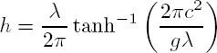
where h is the water depth, c is the celerity, λ is the wavelength and g is the universal gravitational constant. Equation [12.5] is referred to as the dispersion relation. This method was first used in a practice during World War II (Williams 1947).
We provide below some history on this particular satellite-based method. The aim of what follows is to offer an introductory overview of existing studies that have used this same approach (i.e. the time lag due to the satellite sensor geometry). We note that we cannot pretend to be perfect in this bibliographic exercise. Therefore, we do apologize to the authors who might feel excluded.
The use of wave propagation to retrieve shallow bathymetry works either with two sequential images acquired with a short time interval, shorter than a wave period, or with one image, which requires in situ measurement for estimating the wave celerity, as explained by Danilo and Melgani (2016). The retrieval of wave celerity from the satellite is thus a key element and is still challenging today. Access to at least two consecutive images with a few seconds of time delay is crucial to extract bathymetry. As we discussed earlier, this peculiar image acquisition geometry exists onboard specific satellites with pushbroom sensors. With these sensors, the retrieval of c relies on the non-simultaneous stereo acquisition capability of platforms such as Ikonos. To our knowledge, Abileah (2006) was the first to exploit this capability to retrieve coastal bathymetry from Ikonos. Ikonos presents an 11 second time lag between the PAN and the MS sensors, so there may be ambiguity when tracking a wave, depending on its speed. However, the retrieval of c can rely on the fact that two multispectral bands cannot coexist on the focal plane of the instrument, such as in the SPOT family, Pléiades, Sentinel 2 and Landsat 8, yielding de facto a small time lag, sufficient to measure c directly (de Michele et al. 2012). With the joint measurement of c and λ, h becomes accessible from the satellite, without the need for ground calibration. To provide some history of previously published studies, Abileah (2006) suggested a method to measure c from optical satellite data using Ikonos stereo pairs. De Michele et al. (2012) improved the method by using the small time lag between two bands of the SPOT-5 dataset. Danilo and Binet (2013) have detailed the concept and limiting factors. On these bases, Poupardin et al. (2016) proposed local spectral decomposition before the celerity estimates in order to produce local c−λ pairs to derive water depth based on the dispersion relation. Bergsma et al. (2019, 2021) proposed a method based on multiple Sentinel 2 bands and the Fourier slice theorem. Almar et al. (2019) proposed a method to extract c−λ-based bathymetry from Pléiades “persistent” mode. Most of the aforementioned studies make use of only one c−λ couple – the most energetic – to extract bathymetry for a resolution cell, while Poupardin et al. (2016) and de Michele et al. (2021) used multiple c and λ pairs to improve water depth retrieval.
Practically, we consider a sub-section of two bands, normalized by the mean of each sub-section amplitude, resulting in two matrices [A] and [B]. We call this a “window” or resolution cell. With i and j, we can identify the column/line indices in the window. Over a given window, we compute the two-dimensional discrete fast Fourier transform (DFFT) per detector band (matrices [FA] and [FB]). ν and μ are the column/line indices in the Fourier domain. Then, we compute the matrix [R] whose coefficients are given by:
where ∗ represents the complex conjugate and Am is the amplitude of the spectrum. On the module of Rν,μ, we identify multiple peaks that can be considered to be representative of the most significant waves. Then, we can derive their associated wavelengths λν,μ and the phases φν,μ. [A] and [B], being separated in time by 1.05 s, are assumed to have the same spatial frequency content. For this reason, the positions of peaks in ![]() coincide. Therefore, we can identify significant wavelengths in [R]. Finally, we determine c by measuring the pixel offset in the wave motion direction (δrν,μ) between the two bands, which is directly related to the phase of Rν,μ by
coincide. Therefore, we can identify significant wavelengths in [R]. Finally, we determine c by measuring the pixel offset in the wave motion direction (δrν,μ) between the two bands, which is directly related to the phase of Rν,μ by
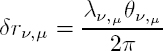
Then, we obtain c by dividing δrν,μ by δtk,l, where δtk,l is the time span between band k and band l. When the pixel offset is not wavelength-dependent (i.e. rν,μ = r, ∀(ν, μ)), this formula (equation [12.7]) is equivalent to the phase correlation algorithm used for earthquake-induced ground-offset measurements (e.g. Puymbroeck et al. 2000). Now, knowing δt, we aim for ((λν,μ), (θν,μ)) pairs that can be converted to ((λν,μ), (θν,μ)). We use the spectral amplitude of R (Am in [12.6]) as a criterion for selecting the most significant waves. This particular method was developed by de Michele et al. (2021) under the framework of the ESA/BRGM-funded BathySent project (2017–2020).
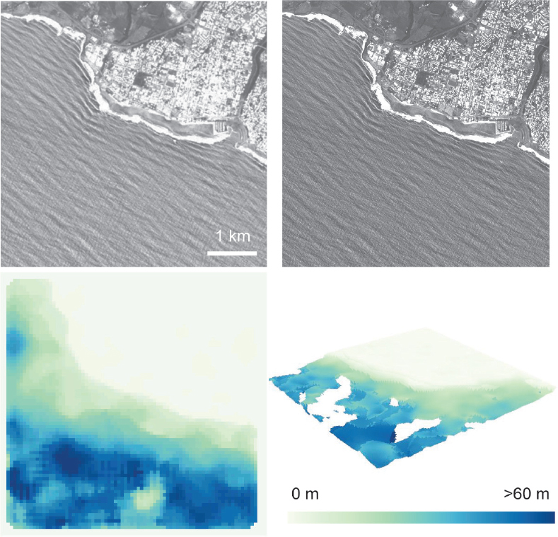
Figure 12.7. Coastal bathymetry from quasi-synchronous SPOT-5 images and linear wave theory. Top: a subset of two SPOT-5 images belonging to the same dataset at 2.05 seconds apart, multispectral on the left and panchromatic on the right. Bottom: the bathymetry retrieved with the BathySent method with SPOT-5 data and a 3D visualization. ©BRGM 2020. For a color version of this figure, see www.iste.co.uk/cavalie/images.zip
12.3.3. Applications
In this chapter, we provide two examples. The first case is based on the CNES SPOT-5 images of La Réunion Island. During a flight, SPOT-5 acquires panchromatic and multispectral images separated by 2.05 seconds, as shown in Figure 12.7. Note how the ocean waves are easily observable in both the images. Also, note how their wavelength decreases, as one approaches the coast. Their celerities also decrease; we could see this here if we could switch back and forth from one image to the other. In the second case (Figure 12.8), we use the EU Copernicus Sentinel 2 to calculate bathymetry. Sentinel 2 focal plane modules are arranged in a staggered geometry. They present useful time lags between multispectral bands for the aims of bathymetry retrieval. Below we show the application of the BathySent method to Sentinel 2 images for the Gulf of Lion (France).
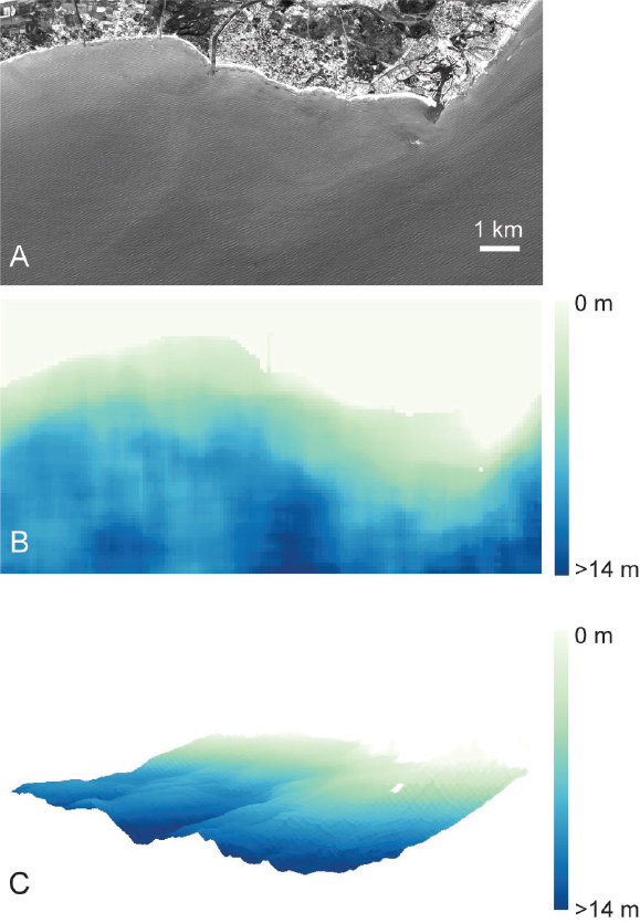
Figure 12.8. Coastal bathymetry derived from Sentinel 2 and wave theory. Computation undertaken at BRGM (2019) under the ESA/BRGM-funded BathySent project. A) Sentinel 2 data acquired for the Gulf of Lion, France. B) Coastal bathymetry retrieved between 0 and 14 meters depth. C) 3D visualization. Figure contains modified Copernicus Sentinel data. ©BRGM 2020. For a color version of this figure, see www.iste.co.uk/cavalie/images.zip
12.4. Concluding remarks
As occurred in the case of SAR and InSAR, sometimes a sensor can be used to extract information in a different manner from the main scope of the mission the sensor was built for. In the field of scientific research, most often, a measurement error (or a bias in a sensor) for one scientist is an invaluable source of information for another scientist. In this chapter, we showed how it is possible to exploit a peculiar characteristic of the focal plane of a high-resolution pushbroom instrument to extract crucial geophysical parameters via conventional cross-correlation techniques based on FFTs. Here, these parameters provide a detailed map of elevation and velocity of a volcanic ash cloud and coastal bathymetry. Frequent image acquisitions, enabled by the joint use of multiple platforms, help to multiply the number of measurements. On the one hand, frequent acquisitions are key to performing multi-temporal analysis of ash plume evolution and ground deformation monitoring under water. On the other hand, they are crucial to improving the precision of measurements through data stacking. Future spaceborne missions will assure the continuity with actual missions and encourage scientists to invest energy in creative research and method development in this field. On the one hand, new high-resolution sensors, such as the Co3D and Pléiades NEO from the CNES, among others, will help in the routine monitoring of the Earth’s surface. On the other hand, the EU Copernicus program, with the Sentinels, will ensure long-term mission continuity, thus providing a solid framework for research and development.
12.5. Acknowledgments
We would like to thank BRGM for supporting these research initiatives. We thank Deborah Idier, Adrien Poupardin, Michael Foumelis (BRGM, France), Þórður Arason (IMO, Iceland), Claudia Spinetti, Stefano Corradini, Luca Merucci (INGV, Italy) and Vivi Drakapoulou (ECMR, Greece) for the scientific contributions. We are thankful to NASA/USGS, Catherine Proy, Claire Tinel (CNES), Espen Volden (ESA) and the Copernicus program (EU) for releasing the satellite data. We thank Céline Danilo and Jean-Marc Delvit for their careful reviews and comments that helped to improve this chapter.
12.6. References
Abileah, R. (2006). Mapping shallow water depth from satellite. Proceedings of the ASPRS Annual Conference, 1–7.
Almar, R., Bergsma, E.W., Maisongrande, P., de Almeida, L.P.M. (2019). Wave-derived coastal bathymetry from satellite video imagery: A showcase with Pleiades persistent mode. Remote Sensing of Environment, 231(111263).
Bergsma, E.W., Almar, R., Maisongrande, P. (2019). Radon-augmented Sentinel 2 satellite imagery to derive wave-patterns and regional bathymetry. Remote Sensing, 11(1918).
Bergsma, E.W., Almar, R., Rolland, A., Binet, R., Brodie, K.L., Bak, A.S. (2021). Coastal morphology from space: A showcase of monitoring the topography–bathymetry continuum. Remote Sensing of Environment, 261, 112469.
Corradini, S., Merucci, L., Prata, A.J. (2009). Retrieval of SO2 from thermal infrared satellite measurements: Correction procedures for the effects of volcanic ash. Atmospheric Measurement Techniques, 2, 177–191.
Danilo, C. and Binet, R. (2013). Bathymetry estimation from wave motion with optical imagery: Influence of acquisition parameters. MTS/IEEE OCEANS Bergen, 10–14 June.
Danilo, C. and Melgani, F. (2016). Wave period and coastal bathymetry using wave propagation on optical images. IEEE Transactions on Geoscience and Remote Sensing, 54(11), 1–13.
Flower, V.J. and Kahn, R.A. (2017). Assessing the altitude and dispersion of volcanic plumes using MISR multi-angle imaging from space: Sixteen years of volcanic activity in the Kamchatka Peninsula, Russia. Journal of Volcanology and Geothermal Research, 337, 1–15.
Kääb, A. and Leprince, S. (2014). Motion detection using near-simultaneous satellite acquisitions. Remote Sensing of Environment, 1154, 164–179.
Mai, S. and Latry, C. (2009). Digital elevation model computation with SPOT5 panchromatic and multispectral images using low stereoscopic angle and geometric model refinement. IEEE International Geoscience and Remote Sensing Symposium, 12–17 July, Cape Town, South Africa.
Massonnet, D., Giros, A., Breton, E. (1997). Forming digital elevation models from single pass spot data: Results on a test site in the Indian ocean. IEEE International Geoscience and Remote Sensing Symposium, 3–8 August, Singapore.
de Michele, M., Leprince, S., Thiébot, J., Raucoules, D., Binet, R. (2012). Direct measurement of ocean waves velocity field from a single SPOT-5 dataset. Remote Sensing of Environment, 119, 266–271.
de Michele, M., Raucoules, D., Arason, P. (2016). Volcanic plume elevation model and its velocity derived from Landsat 8. Remote Sensing of Environment, 176, 219–224.
de Michele, M., Raucoules, D., Corradini, S., Merucci, L., Salerno, G., Sellitto, P., Carboni, E. (2019). Volcanic cloud top height estimation using the plume elevation model procedure applied to orthorectified Landsat 8 data. Test case: 26 October 2013 mt. Etna eruption. Remote Sensing, 11(785).
de Michele, M., Raucoules, D., Idier, D., Smai, F., Foumelis, M. (2021). Shallow bathymetry from Sentinel 2, by joint estimation of waves celerities and wavelengths. Remote Sensing, 13(2149).
Nelson, D.L., Garay, M.J., Kahn, R.A., Dunst, B.A. (2013). Stereoscopic height and wind retrievals for aerosol plumes with the MISR interactive eXplorer (MINX). Remote Sensing, 5, 4593–4628.
Pailot, S., Bonnétat, S., Harris, A., Calvari, S., de Michele, M., Gurioli, L. (2020). Plume height time-series retrieval using shadow in single spatial resolution satellite images. Remote Sensing, 12(3951).
Poupardin, A., Idier, D., de Michele, M., Raucoules, D. (2016). Water depth inversion from a single SPOT-5 dataset. IEEE Transactions on Geoscience and Remote Sensing, 54, 2329–2342.
Prata, A.J. and Grant, I.F. (2001). Retrieval of microphysical and morphological properties of volcanic ash plumes from satellite data: Application to Mt Ruapehu, New Zealand. Quarterly Journal of the Royal Meteorological Society, 127, 2153–2179.
Prata, A.J. and Turner, P.J. (1997). Cloud top height determination from the ATSR. Remote Sensing of Environment, 59(1), 1–13.
Puymbroeck, N.V., Michel, R., Binet, R., Avouac, J.-P., Taboury, J. (2000). Measuring earthquakes from optical satellite images. Applied Optics, 39, 3486–3494.
Scollo, S., Folch, A., Coltelli, M., Realmuto, V.J. (2010). Three-dimensional volcanic aerosol dispersal: A comparison between multiangle imaging spectroradiometer (MISR) data and numerical simulations. Journal of Geophysical Research, 115(D24210).
Spinetti, C., Barsotti, S., Neri, A., Buongiorno, M., Doumaz, F., Nannipieri, L. (2013). Investigation of the complex dynamics and structure of the 2010 Eyjafjallajökull volcanic ash cloud using multispectral images and numerical simulations. Journal of Geophysical Research, 118(10), 4729–4747.
Vadon, H. (2003). 3D navigation over merged panchromatic-multispectral high resolution SPOT5 images. Proceedings of the 2003 ISPRS Symposium.
Williams, W.W. (1947). The determination of gradients on enemy-held beaches. The Geographical Journal, 109(1–3), 76–90.
Wilson, L., Sparks, R.S., Huang, T.C., Watkins, N.D. (1978). The control of volcanic column heights by eruption energetics and dynamics. Journal of Geophysical Research, 83(B4), 1829–1836.