
1
Relevant Past, On-going and Future Space Missions
Philippe DURAND and Stephane MAY
CNES, Toulouse, France
Earth observation satellites have provided images all around the world for more than half a century. Passive optical imaging systems and synthetic aperture radar (SAR) active sensors are nowadays the main sources of information used to derive surface displacement fields. To provide an overview of the images available through space agencies and their main characteristics, this first chapter describes different space missions with data relevant for ground motion displacement measurements. For radar, it is important to observe the field under the same incidence angle, meaning that this may depend upon the satellite orbit housekeeping and general design. SAR missions where orbit is not maintained are not mentioned (except the Iceye mission): their data seem useless at first sight for SAR interferometry (InSAR, see Chapter 4) and probably for SAR correlation algorithms (offset tracking, see Chapter 3). Data access, particularly when free of charge, is also described for the missions.
1.1. Some key parameters for space missions
1.1.1. Parameters for both SAR and optical missions
Remote sensing missions to date have had low-altitude orbits of a few hundred kilometers around the Earth. While optical missions mainly work, except for infrared instruments, along half of the orbit under sun lighting, SAR images can be acquired across the whole orbit, day and night, and also through cloud cover for the frequencies examined later in this chapter.
Sun-synchronous missions: Most remote sensing missions are placed on sun-synchronous orbits. This is important for optical imagery to assure the same looking angle with regard to the sunlight (although it slightly changes anyway with the seasons). These orbits are also used for SAR imagery, sometimes because they are on the same platform as optical sensors (e.g. JERS-1, Envisat or ALOS), and also because of power constraints. Radar instruments have high power consumption and thus recent missions are often on a 6:00 and 18:00 (or dawn–dusk) orbit that maximizes the energy received by a solar panel (which can be fixed and always orientated towards the sun). ERS-1 and ERS-2 inherited a platform heritage from the first French optical satellite (SPOT-1), keeping the local hour at 22:30 (10:30 descending): the panel had a fixed direction towards the sun but had to make one rotation per orbit on the spacecraft.
These orbits are also near polar orbits, which assure a large coverage of the Earth, except some areas near the poles, depending on the look angle and swath, and with differences between the south and north poles depending on whether the radar is left- or right-looking. When crossing the equator, these orbits have a fixed local hour, which must be maintained throughout the mission duration (inclination maneuvers): this is a key parameter, and all satellite passes occur at the same hour if observed under the same incidence angle. Note that the reference value of the local hour is when the orbit crosses the equator from south to north (ascending part).
Revisit: This corresponds to the time taken for a satellite to revisit a given geographical location on the Earth. It depends on the satellite orbit (altitude, inclination, etc.) and agility.
Repeat cycle: This key parameter expresses the number of days separating two data takes under the same orbital point of view, which can be equal to or higher than the revisit. At the beginning of the mission, in relation to the sensor field of view or swath, we must establish a total number of orbits Ntot and also choose the number of days in the cycle Dcycle. Then, we have the following relationship:
where [14(or 15) + p/Dcycle] is the number of orbit revolutions in one day. The orbit duration is about 100 min as the orbit altitudes are in the range of 400–900 km: when under 96 min, there will be at least 15 orbits/day. p is an integer chosen with a close relationship to Dcycle.
It is possible to change the repeat cycle during a mission, which means a change of altitude for the satellite. For example, ERS-1, with a change of altitude of less than 6 km, had a Dcycle that changed from 35 to 3 days. With a constellation where all satellites have the same orbit (but are phased differently), for example, with SPOT, ERS, CSK, Sentinel and TerraSAR-X/TanDEM-X/PAZ constellations, it is possible to combine images from the different satellites and hence reduce the time interval between data takes while keeping the same orbital point of view, called the “repeat time”.
Table 1.1. Main orbital parameters for some sun-synchronous SAR missions
| Satellite | Local hour | Entire rev. | p | Dcycle (days) | Ntot | Altitude (km) |
| ERS-1, ERS-2 routine | 22:30 | 14 | 11 | 35 | 501 | 785 |
| ERS-1 phases A, B, D | 22:30 | 14 | 1 | 3 | 43 | 775 |
| Envisat | 22:30 | 14 | 11 | 35 | 501 | 785 |
| Envisat end of life | 22:30 | 14 | 11 | 30 | 431 | 783 |
| Radarsat-1,2 | 18:00 | 14 | 7 | 24 | 343 | 798 |
| JERS-1 | 22:30 | 14 | 43 | 44 | 659 | 568 |
| ALOS | 22:30 | 14 | 27 | 46 | 671 | 692 |
| TerraSAR-X, TanDEM-X, PAZ | 18:00 | 15 | 2 | 11 | 167 | 515 |
| CSK, CSG | 6:00 | 14 | 13 | 16 | 237 | 620 |
| Sentinel-1A/B | 18:00 | 14 | 7 | 12 | 175 | 693 |
| Radarsat CM | 18:00 | 14 | 11 | 12 | 179 | 593 |
| ALOS-2 | 18:00 | 14 | 3 | 14 | 199 | 628 |
Table 1.2. Main orbital parameters for some sun-synchronous optical missions
| Satellite | Local hour | Ascending/descending | Period of orbit (min) | Dcycle (days) | Altitude (km) |
| Cartosat-2A/2B | 9:32 | D | 97.4 | 5 | 635 |
| Landsat 8 | 10:00 | D | 98.8 | 28 | 705 |
| SPOT-7 | 10:30 | D | 98.8 | 26 | 694 |
| Sentinel-2A/2B | 10:30 | D | 100.6 | 10 | 786 |
| Kompsat-3A | 10:50 | A | 95.2 | 28 | 528 |
| Co3D | 11:00 | - | 94.6 | - | 502 |
| WorldView-1 | 13:30 | D | 94.6 | 14 | 496 |
| Eros B | 14:00 | D | 94.8 | 4 | 520 |
Common parameters for optical missions: For the optical missions, the same orbital parameters are key elements for the mission. The orbits are in general sun-synchronous. The local hour has a direct impact on the viewed scenes. There is a compromise between viewing a scene early in the morning in order to reduce atmospheric effects (water vapor) and near midday in order to reduce the length of shadows in the images. The local hour is in general chosen between 9:30 and 14:00.
The choice of the orbital altitude has an impact on the spatial resolution, as well as on the viewing angle of the terrestrial scenes if a high revisit rate is required. High-resolution satellites are, in general, agile and consequently relax the mission constraints. The altitude of low Earth orbit (LEO) satellites is, in general, chosen to be between 420 km, the altitude of the International Space Station (ISS), and 900 km. The final resolution of the disparity map used to derive elevation (see Chapter 2) or offset map used to derive displacement is directly linked to the initial image resolution. So, the spatial resolution of the pixels is one of the key parameters of an optical mission.
Non-sun-synchronous missions: The famous Shuttle Radar Topography Mission (SRTM) was phased, but not sun-synchronous. With an inclination of 57° at 233 km altitude, this mission produced a worldwide digital elevation model (DEM), but it was limited in latitude.
1.1.2. Parameters specific to SAR missions
This section addresses some parameters specific to SAR systems. Some important parameters, such as the range and azimuth ambiguity ratios, are not listed because they do not really affect phase or ground motion measurements.
Central frequency and bandwidth: In SAR remote sensing, frequency allocation is a key issue. The International Telecommunication Union Radiocommunication Sector (ITU-R) provides recommendations for remote sensing (ITU-R 2009), and particularly for active microwave sensors with regard to Radiocommunication Requirements (RR) Art. 5 (Table 1.3).
Table 1.3. Allocated frequencies and bandwidths for active SAR civil sensors in space as mentioned by the ITU-R (2009)
| Allocated frequencies by RR Art. 5(MHz) | Conventional letter | ITU required bandwidth (MHz) |
| 432–438 | P | 6 |
| 1,215–1,300 | L | 20–85 |
| 3,100–3,300 | S | 20–200 |
| 5,250–5,570 | C | 20–320 |
| 8,550–8,650 | X | 20–100 |
| 9,300–9,900 | X | 20–600 |
There are concerns, however, about other ITU attributions that affect these frequencies, in particular in the C-band (wireless LAN, mobile phones) and L-band (radio location and radio navigation), according to the ITU-R (2010). Sometimes military radars are also active in such frequencies. Both can cause real interferences in image data and make them partly useless. Each frequency has its own properties, and all categories have either flown (L, S, C, X) or are being scheduled (P-band with Biomass).
We can note from Table 1.3 that the highest bandwidth is available in the X-band: as a result of this point combined with the more compact antennas needed for such missions and the inferred cost reduction, many new satellites are aiming at the X-band. In the ITU WRC 2015 meeting, an extension to a 1,200-MHz bandwidth (9,200–10,400 MHz) was approved, but some countries have expressed reservations and stick to 9,300–9,900 MHz (ITU-R 2020). In addition, this table is not applicable everywhere: for instance, the P-band is not accepted over the United States for SAR civil sensors. SAR missions of the interest detailed in this chapter and associated frequency bands are listed in Figure 1.1.
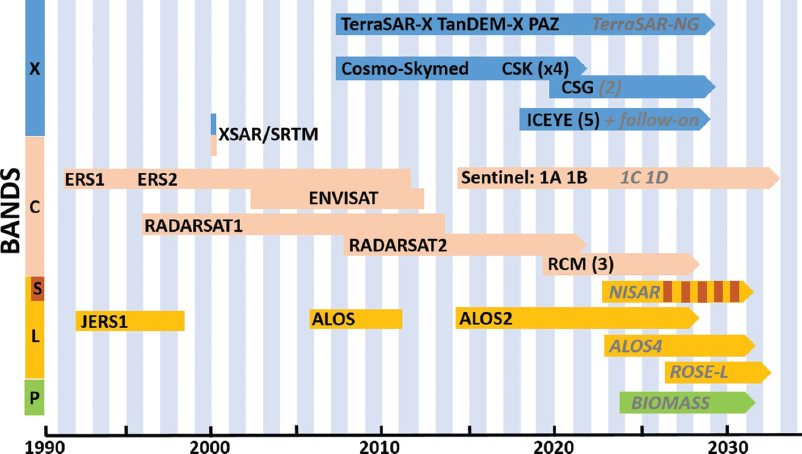
Figure 1.1. Relevant SAR missions and associated frequency bands (future missions in gray italics). For a color version of this figure, see www.iste.co.uk/cavalie/images.zip
Radar swath and pulse repetition frequency (PRF): Stripmap is the simplest working mode of a SAR system. More advanced modes can be explained relative to this mode. In stripmap, the resolution after synthesis in the azimuth direction (along-track) is given by half the antenna length La/2. The Doppler bandwidth in the azimuth is given by BDop = vs/c/(La/2), where vs/c is the satellite velocity. The PRF fP needs to be higher than BDop to avoid spectral layover in the azimuth. In contrast, in the range direction (across-track), the PRF must be limited to avoid range ambiguities or, to put it another way, the swath will be maximized if the PRF is minimized: swath < c/2fP . This explains why stripmap swath is lower in X-band compared to C-band missions (a shorter antenna means higher PRFs and narrower swaths).
If higher resolution is needed, it is possible to expand BDop by electronic steering in the azimuth (the same resolution is kept in range) and thus to increase the length of observation along the orbit: this is called the spotlight mode. The counterpart is that it is no longer possible to obtain a continuous along-track imaging as in stripmap, but only sparse scenes. If a larger swath is needed, then the approach is to use ScanSAR modes: the Doppler bandwidth is shared between different subswaths. By adding an azimuth steering mode like a “reverse” spotlight, it is possible to obtain a Sentinel-1-like mode called the terrain observation by progressive scan (TOPS) mode (Zan and Guarnieri 2006). The range resolution can stay the same as the stripmap mode. In some missions with multi-incidence angles (Envisat or Radarsat-1, for instance), loss of range resolution has been mitigated for some modes by increasing the transmitted bandwidth to assure a better ground-range resolution for the lowest incidence angles.
Yaw steering: Most SAR missions use yaw steering on board, so that the spacecraft compensates for Earth rotation and the point perpendicular to the orbit is effectively at zero Doppler. Radarsat-1 was not yaw steered, which resulted in a Doppler shift of several PRFs.
Incidence angle: In contrast to optical sensors, SAR imaging sensors cannot look to the nadir, as this would create simultaneous echoes in the same pixel from both sides. In addition, the best resolution is obtained at the largest incidence angle, at the expense of lower power received due to the increased distance from the ground. The choice of the incidence angle is critical in mountainous areas due to layover on one side and shadows on the other side of mountains.
Orbit precision: This is an important parameter used to combine SAR images for interferometry. An orbit that is not precisely known will lead to an important phase gradient in the interferogram. There are three kinds of orbit that can be successively delivered:
- – the first is a predicted orbit that usually comes along with the product when produced in real time;
- – then, a few hours or days after the data acquisition, a restituted orbit is available with more precision;
- – finally, after three or four weeks, the most precise orbit can be delivered to users, thanks to dedicated payloads and specific computing.
Nowadays, with precise orbit determination payloads onboard, orbit precision can be known at the order of a few centimeters.
Orbital tube: Recent SAR missions have integrated the use of differential interferometry in their specifications (Sentinel-1, ALOS-2, the Radarsat Constellation mission) and have put constraints on orbit housekeeping. Thus, the orbit must stay in a tube called the “orbital tube”, with a radius as small as one hundred or a few hundreds of meters to keep the perpendicular baseline small (see Chapter 4, section 4.2).
Duty cycle, down-link rate and onboard storage: The duty cycle is equivalent to the percentage of time that the radar will be able to work along the orbit. SAR systems need a lot of energy, making it impossible for them to work permanently. Depending on the design of the satellite power unit, a system can deliver between a few seconds of imaging and about 1/4 of the orbit time. There is a huge difference between very small satellites of a few hundreds of kilograms and big platforms of two or three tons. The down-link rate and onboard storage capacity are often two key elements that usually come together. A data relay satellite is sometimes helpful to cope with all the constraints or avoid multiple ground antennas for down-linking, but this usually needs a laser link and data relay commercial contract, which can also be quite expensive.
Instrument noise equivalent σ0: This parameter is very important when looking at amplitude images. It gives the minimum value that can be reached by the system for an elementary pixel, but entails lower values with multi-looking (see Chapter 3). It varies in range along the swath, and the specification must deliver the worst case: in general, the best values are in the middle of the swath where the antenna gain is maximum. This parameter affects measurements for ground motion: if its value is too poor, then some surfaces that have low backscattering coefficients will not be properly estimated, for instance asphalted roads, tarmacs and even sand in the desert.
Polarization: The design of the antenna sub-system determines what polarization should be implemented. For ground displacement purposes, as the signal-to-noise ratio (SNR) is more favorable, co-polarized data are mainly used, and it is difficult to say whether using HH and VV for offset tracking or InSAR techniques are more advantageous. The use of dual polarization, HH+HV or VV+VH, or quad polarization (HH+HV+VV+VH) is more relevant for other remote sensing applications, such as classification, forest extents and heights, maritime surveillance, pollution at sea or other change detection characterizations. Furthermore, the use of quad polarization generally reduces the swath and azimuth resolution by a factor of two, and thus the size of the archive in this mode is less important.
1.1.3. Parameters specific to optical missions
Pushbroom: A pushbroom camera consists of an optical system projecting an image onto a linear array of sensors. Usually, a focal plane is composed of several time delay integration (TDI) image sensors, mounted in a staggered configuration. The image is directly built at the sensor level. Charge-coupled device (CCD) sensors are used where ultra-low noise is preferred, and now complementary metal oxide semiconductor (CMOS) matrix detectors are increasingly used.
Stereo, tri-stereo and more: To build a disparity map (see Chapter 2), at least two stereo images from separate view angles are necessary. It is possible to combine more images (tri-stereo or even more) to build a more precise map. With four images, all faces of buildings may be seen, and it is possible to build a digital elevation model and associated pixel values. The different images over a geographical point are taken from different incidence angles. If they are taken with the same satellite, then they will be asynchronous. If they are taken with a constellation of satellites on the same orbit, then they may be synchronous, such as with the Co3D system. Asynchronous images imply two acquisition instants. If the delay is a few seconds, mobile elements (such as terrestrial vehicles, bots, planes) or clouds will alter the raw displacement measure. If the delay is a few weeks or months, some buildings may appear or disappear. Evolution of agricultural landscape will also alter the match between the images.
Agile satellites: The agility of satellites is a key function. Agile satellites are able to do attitude maneuvers and focus on one scene. This increases the revisit frequency over the same region, and so reduces the time interval between two acquisitions. Such satellites are able to point towards a geographical point thanks to steering mirrors or by changing their whole attitude (yaw, pitch and roll control).
Base-to-height (B/H) ratio: The shift between two images creates a stereoscopic parallax in one direction (see Chapter 2). The stereoscopic angle (also called the base-to-height or B/H ratio) is the ratio between:
- – the distance between the two viewing points (base – B);
- – and the distance to the observed scene (height – H).
In the older generation of satellites, the B/H ratio was directly fixed with the instrument characteristics. For example, the SPOT-5 satellite had high-resolution HRS instruments to provide large-area along-track stereoscopic images (forward and backward of the satellite). With agile satellites, it is possible to choose the best view conditions and define the choice of B/H ratio. A large B/H ratio favors the observation of different points of view of the scene (e.g. two faces of buildings) but creates constraints on the disparity computation, as some elements of one scene are not seen in the other one. With a lower B/H ratio, the delay between two images is reduced and a scene can be observed under nearly the same conditions, but it adds constraints to the precision of the disparity computation algorithms. In the case of SPOT-5, the shift between panchromatic and XS detectors (19.5 mm in the focal plane) creates a slight stereoscopic angle that allows a stereo reconstruction using the P+XS correlation. In the case of Pléiades, the B/H ratio is chosen by the user.
The key optical parameters of satellite systems are explained in the following:
Spatial resolution: Spatial resolution is a measure of the smallest angular or linear separation between two objects or two pixels on the ground. It is usually expressed in radians or meters. Spatial resolution decreases as the viewing angle increases. Spatial resolutions are, in general, given at the nadir of the satellite. For example, for Ikonos, the spatial resolution is equal to 0.82 m at the nadir and 1 m at 26° off-nadir.
| Satellite | Mission characteristics | B/H ratio |
| SPOT-5 | Steering mirror (MCV). Stereoscopic angle up to 54 deg | 1.02 |
| SPOT-5 | HRS instrument: angle 40 deg, delay 90 s | 0.8 |
| Co3D | Synchronous acquisitions | 0.20–0.30 |
| SPOT-5 | PAN–XS stereoscopic angle: delay 2.25 s | 0.018 |
| Pléiades | Satellite agility – stereo or tri-stereo | 0.10–0.20 |
| WorldView-3 | Satellite agility – stereo or tri-stereo | B/H = 0.20–0.40 |
Spectral resolution or spectral bands: A ground feature or target is defined by its reflectance and spectral emissivity curve. Its response depends on the wavelength ranges. Different classes of objects in an image can thus be distinguished by comparing their responses over distinct wavelength ranges. A large spectral band captures more signal energy and thus enhances the SNR of the image. A panchromatic band defines a wide spectral band, with high SNR and high resolution. In contrast, a multispectral band (XS) captures specific wavelength ranges separated by filters or instruments sensitive to particular wavelengths: the received signal energy decreases as the bandwidth decreases, and therefore the satellite system is designed with a lower resolution to maintain an acceptable SNR. For a given satellite system, regardless of the spectral bands, disparity estimations are performed with the bands that have the highest spatial resolution and the best SNR. Spectral bands may be separated into several families or groups: thermal infrared (TIR) and medium-wavelength infrared (MWIR) depend not only on solar illumination but also on emission from the imaged objects themselves.
Swath: Swath is the geographical width of the image, which is linked to the optical instrument and the number of detectors in the sensor.
Viewing angle/incidence angle: The viewing angle (satellite point of view) is the angle between the nadir point and the angle towards the terrestrial point. The incidence angle (region point of view) is the angle between the vertical to a point and the direction of the satellite. Thanks to steering mirrors or the agility of the whole satellite, it is possible to modify acquisition angle configurations. A low incidence angle (region near the satellite nadir) means that, for example, only roofs can be seen. With a high incidence angle, building facades can be seen, but some occlusion occurs (hidden faces, hidden streets, etc.). Spatial resolution decreases as the viewing angle increases. Hence, spatial resolutions are given at the nadir of the satellite.
Impact of the spatial resolution: The spatial resolution of the satellite directly drives the analysis that can be performed with the images. The definition of optical missions (HR, VHR, etc.) depends on the spatial resolution:
- – 1,000–3,000 m: Analysis of the atmosphere, aerosols and land surface emissivity/temperature. For example: MSG, METOP;
- – 250–1,000 m: Analysis of the atmosphere, aerosols, land surface emissivity/temperature. For example: MODIS, Sentinel-3;
- – 30–60 m: Analysis of land cover (agriculture, forestry, cartography, geology, cryosphere, etc.). For example: Landsat1–7;
- – 15–20 m (medium resolution (MR)): Analysis of large-scale land cover, agriculture, forestry and highway infrastructures and computation of digital terrain models. For example: Sentinel-2 (red edge, shortwave infrared – 20 m);
- – 1.5–10 m (high resolution (HR)): Analysis of land cover, agriculture, regional to city-level coverage, road infrastructures, digital elevation model extraction and medium or large objects, such as boats, and computation of digital terrain models. For example: SPOT-6–7, Sentinel-2 (blue, green, red, near-infrared – 10 m);
- – 0.5–1 m (very high resolution (VHR)): Analysis of many objects in the images. At this resolution, a large number of objects are visible, such as urban elements, houses, vehicles, buildings affected by natural disasters and archeological objects. Extraction of digital surface models can also be undertaken. For example: Pléiades;
- – < 0.5 m (ultrahigh resolution (UHR)): Detailed analysis of elements of the scene. Many objects are visible in the images with more details, including small vehicles, buildings, archeological objects, etc. Computation of digital surface models can be undertaken. For example: WorldView-3, Cartosat-2.
The main optical satellites that are used for DEM extraction have spatial resolutions better than 10 m. For precise estimation of DEMs, submetric satellites are the best candidates.
Resolution versus swath versus revisit time: The size of telescope mirrors was the limiting factor in reaching high resolutions for the first generations of optical satellites. With the evolution of space technology, the first civil satellites were launched at the beginning of the 2000s with resolutions lower than 1 m. Ikonos was launched in September 1999 and was the first commercial satellite with a resolution of less than 1 m; it was followed by satellites such as Quickbird-2, Eros B, Kompsat-2 and WorldView-1. A satellite with a very high resolution has a reduced swath, in contrast to decametric resolution satellites. A medium-resolution satellite usually has a wider swath and a shorter revisit time. Conversely, meteorological satellites such as the Meteosat Second Generation (MSG) and Meteorological Operational Satellite (MetOp) family usually have a low spatial resolution around 1 or 3 km, with a wide swath between one and several thousands of kilometers, in order to give a view of the meteorological situation. The number of spectral bands, from 500 nm to 15,000 nm, allows a fine analysis of clouds and aerosols. These satellites have a low spatial resolution but a high temporal resolution. Their spatial resolution is not compatible with DEM extraction.
Choice of the spectral bands: The choice of spectral bands combined with the spatial resolution directly drive the applications of a satellite. Many satellite systems exist with many different configurations (PAN+XS configuration, only PAN configuration, only XS configuration, etc.). A significant number of UHR and VHR satellites have four bands (blue, green, red and near-infrared) associated with a panchromatic band. The panchromatic band (P or PAN) usually has a spatial resolution four times higher than the multispectral ones (XS). Pan-sharpening techniques are employed in order to build panchromatic plus multispectral (P+XS) products, which means fused multispectral products at a panchromatic spatial resolution.
| Band name | Spectral interval |
| UV band | 300–400 nm |
| Visible bands (VIS) | 400–700 nm |
| Near-infrared (NIR) bands | 700–1,000 nm |
| Short-wavelength infrared (SWIR) | 1,000–2,500 nm |
| Medium-wavelength infrared (MWIR) | 3,000–5,000 nm |
| Thermal infrared (TIR)/long-wavelength (LWIR) | 8,000–15,000 nm |
High-resolution (HR) satellites work with lower resolution but include additive infrared bands useful for land cover, water color or atmospheric analysis. To compute digital elevation models and to measure displacements, the spectral band with the highest spatial resolution and the best SNR is generally chosen. For many satellites, this is usually the panchromatic band. For some HR systems with only XS bands, multispectral bands may be used (e.g. Sentinel-2).
1.2. Past and on-going SAR missions
This section presents spaceborne missions that have been used or are used to compute displacement fields by interferometric processing. Some peculiarities or issues are pointed out to help the reader understand them. This is thus not an exhaustive list of SAR space missions. Note that the Magellan mission began to map Venus in September 1990 with an SAR instrument, but its topography was computed using a radargrammetry technique, combining two images from either the same side or from opposite sides: this is rather far from the topic of this book, and thus this very successful mission will not be further detailed here. We must note that most of these missions were organized and designed before the interferometric technique emerged, around the beginning of the 1990s. Thus, certain constraints, such as orbit housekeeping, yaw steering and burst synchronization for ScanSAR modes, were sometimes not taken into account in the designs of the spacecraft or payload.
After a series of C-band and L-band satellites at medium resolution in the 1990s, a new generation of SAR satellites operating in the X-band arrived in Europe at the national level (Germany, Italy, Spain) from mid-2007 onwards: although targeting different goals, they all had significantly improved resolutions and repeat pass capacities, which gave them serious advantages when focusing on localized areas.
With small satellite missions, such as ICEYE, interferometry is usually possible with a short time period: maintaining a small orbital tube is too expensive for the length of the mission and archives on large scales are out of scope; however, such constellations can gather significant data over cities and PS techniques can be considered. NovaSAR is not addressed here, as it is a single satellite on a short-term mission with limited applications for interferometry. Some Chinese and Indian missions are also not addressed due to the limited availability of the datasets. Finally, a significant improvement in interferometric abilities and coverage arrived with missions such as Sentinel-1 and ALOS-2.
1.2.1. ERS-1, ERS-2 and Envisat
ERS-1 (1991–2000) and ERS-2 (1995–2011), the European remote sensing satellites, began the era of SAR instruments in Europe and demonstrated the first applications in radar interferometry. The five-year overlap provided the opportunity to develop very nice orbital combinations, such as the so-called tandem phase, allowing acquisitions of the same area within just a one-day interval, which was much more favorable than the native 35-day repeat cycle for InSAR on rapidly changing surfaces.
The Environmental Satellite (Envisat) continued the C-band SAR missions for Europe with the ASAR instrument, as well as numerous added payloads, among which were the DORIS instrument for precise orbit determination and the MERIS spectrometer, giving simultaneous information on the composition of the atmosphere and overlapping most of the SAR swath. Envisat was put on the same 35-day orbit as the ERS series from April 2002 until October 2010, when a drifting orbit had to be set due to the lack of propellant until its end in May 2012.
ERS-2 had an overlap in the years 2007–2008 with Envisat, with a 30 min delay between the two satellites, but the central frequency was shifted from 5.3 GHz (ERS) to 5.33 GHz (Envisat) so that cross-intereferometry was restricted to common bandwidth in limited cases.
The geometry of ERS satellites was quite simple with a 23° fixed incidence angle, swath of about 100 km and one single polarization set to VV. The Envisat ASAR instrument was more complex, with modes divided in ScanSAR and its large swath of 405 km (composed of five sub-swaths), as well as seven stripmap modes (IS1 to IS7). A wave mode was operated over the ocean. Customers could order any kind of mode, so the archive was not homogeneous over the Earth and strongly depended on the area considered: it therefore became more difficult to get two images acquired in the same mode, suitable for interferometry. However, for some closely monitored volcanic islands, it was quite interesting to get different passes in the 35-day cycle with different incidence angles.
Note also that ASAR was not full polarimetric, but authorized different kinds of scheme, such as the alternating polarization (AP) mode, which could emit alternatively in H and V polarizations and receive H and V.
Some limitations of the missions with regard to interferometry: As these missions were decided before differential interferometry emerged, some limitations had to be tackled (Solaas and Coulson 1994). For ERS-1/2, orbital housekeeping looseness led to perpendicular baselines B⊥ (see section 4.2.2 in Chapter 4) higher than the limit of 1,100 m. A preferred value of 600 m was set for B⊥ (see definition in section 4.2), so that a tool to determine which orbits or track frames were compatible for interferometry had to be developed. In addition, the orbit was not known as precisely as the latest SAR missions: orbital fringes had to be removed before interpretation. PRARE, a dedicated instrument for precise orbit determination, failed after several weeks on ERS-1 but lasted several years on ERS-2 and was able to deliver precise ranging accuracy of less than 7 cm.
In contrast to future missions (e.g. ALOS-2 or Sentinel-1), Envisat ScanSAR bursts were not synchronized on board, meaning the Doppler overlaps had random values from one pass to another and were not always compatible. Some results were however published in ScanSAR mode; for instance, for the 2003 Bam earthquake in Iran.
In late October 2010, Envisat got a new orbit cycle of 30 days in a degraded configuration. At this point, interferometry could only work around latitudes of 38° (north and south). As a result, tracks could not be combined with the previous 35-day orbit cycle. However, along-track interferometry in the new geometry could produce interesting results, for example interferograms for the Sendai (Tohoku) earthquake that occurred on March 11, 2011, which led to the Fukushima disaster.
Data access: During the missions, European Space Agency (ESA) products were not free of charge and RAW data were much cheaper. Furthermore, some technical teams preferred to do the radar synthesis themselves to ensure a better signal shape in the range spectrum. Nowadays, as indicated by the ESA (2019), the (A)SAR on-the-fly (OTF) data processing and dissemination service allows end-users to gain direct access to ESA’s complete high-resolution (A)SAR archive from the ERS-1, ERS-2 and Envisat missions. The service provides (A)SAR Level 1 high-resolution data, which are processed from Level 0 on user request by the system. Users can register themselves and immediately download Level 1 (A)SAR data products. The service is available via the ESA Online Dissemination Service at https://esar-ds.eo.esa.int/oads/access.
1.2.2. Canadian C-band satellites: Radarsat-1, Radarsat-2 and RCM
Radarsat-1 was the first imaging radar developed for the Canadian Space Agency (CSA). It was launched in December 1995 and ended its operations in April 2013. The satellite had noticeable activity over the Arctic areas for ice monitoring. In the late 1990s, it was the only civilian radar capable of imaging part of the Earth, while ERS could only operate in the visibility of ground receiving stations due to the lack of onboard recording. The satellite offered a variety of imaging modes, including the large swath in ScanSAR (510 km) and narrow ScanSAR (305 km), seven stripmaps (100 km) and three others with 150 km swath, ranging from 20 to 47°, as well as 15 fine modes at incidences above 37° (45 km). The radar operated only in single co-polarization HH. The satellite native design was right-looking imaging, but the CSA conducted a dedicated campaign over Antarctica with a 180° rotation of the spacecraft, making it left-looking, and the first radar mosaic of the continent could thus be produced. Interferometry was demonstrated during the mission, although there were some strong limitations with this spacecraft. Radargrammetry for DEM was also demonstrated, prior to the SRTM mission.
There were several limitations of the mission with regard to interferometry:
- – the satellite was not yaw-steered, meaning the Doppler centroid had strong values, exceeding several PRFs, as well as strong variations in the year, and for interferometry, we should take care when combining pairs, the minimum and maximum of Doppler shift being around the solstices;
- – the orbit-keeping was quite loose, and baselines reached several kilometers;
- – orbital knowledge was a special issue in computing correct interferograms, and the use of fine orbit interpolators, such as Hermite polynomials, was a necessity.
The Radarsat-2 spacecraft was launched in December 2007 while Radarsat-1 was still operating. The spacecraft added significant improvements in many areas: right-and left-looking, quad polarization, low σ0, ultrafine modes, ground track maintained within a 500 m wide range, yaw steering and onboard state recorders. Although on the same reference orbit as Radarsat-1, Radarsat-2 images were not pairable with Radarsat-1 for interferometry: the central frequency was shifted from 5.3 to 5.405 GHz and the Doppler centroid was not compatible, due to the difference in yaw steering. At the end of 2020, the spacecraft was still operating, making a transition to the next Canadian SAR mission.
The Radarsat Constellation Mission (RCM) aims to replace the Radarsat-2 mission, continuing the traditional Canadian C-band SAR imagery as well as adding automatic identification system (AIS) payloads to improve maritime surveillance. It is composed of three identical satellites that were launched together in June 2019 for an expected lifetime of seven years. The sun-synchronous constellation has a 18:00 ascending node and flies at an altitude range between 586 and 615 km. As the three satellites are equally spaced along the orbit, the repeat time is only four days, and the orbit is maintained within a 120 m radius orbital tube, which gives good advantages for several InSAR applications. Various schemes of polarization are implemented: single polarization, dual co-cross or compact polarimetry are available on all modes; dual HH–VV is available for specific modes, as well as a quad-polarization mode. Radar modes are numerous, from spotlight (1×3 m resolution, one look) to wide ScanSAR (100 m, eight looks)
Data access: Since April 2019, 36,000 images of archive data acquired by the Government of Canada all over the world have been freely available (see CSA 2019). Unfortunately, not all acquired data can be accessed at the time of editing (2021).
1.2.3. Japanese L-band satellites: JERS-1, ALOS and ALOS-2
The Japanese Earth Resources Satellite (JERS-1) was the first of a series of Japanese SAR sensors working in the L-band, followed later by the Advanced Land Observing Satellite (ALOS) and ALOS-2. All three projects were conducted under governmental institutions. Launched in February 1992, JERS-1 lost its onboard recording capacity in August 1997, which limited its use over direct receiving ground stations, and the spacecraft finally terminated its mission in October 1998. The SAR sensor operated at 1.275 GHz (wavelength of 23.5 cm), with a bandwidth of 15 MHz. Only co-polarization in HH was implemented. The nominal swath was a stripmap mode of 75 km, at a fixed look angle of 35°. Tracks were acquired regularly, minimizing the time between two consecutive swaths, which was a great advantage for large mosaics and radiometric stability. Interferometry showed great coherence for vegetated areas compared to C-band radar, as in ERS, with comparable resolution. As an optical system (OPS) was also used, the satellite was put on a sun-synchronous orbit with a descending node at 10:30 to 11:00.
ALOS was the second Japanese satellite and was able to deliver L-band SAR images through its PALSAR instrument operating at a 1,270 MHz central frequency. The launch took place in January 2006, and the local hour was set at 10:30 descending node, with an onboard optical sensor (PRISM, AVNIR-2). The bandwidth was increased to 28 MHz in single-polarization HH or VV and 14 MHz in dual-polarization HH+HV VV+VH or quad polarization with different fine beams, with 70 km and 40 km swath, respectively. The ScanSAR mode only worked in co-polarization HH or VV, with a 350 km swath sub-divided into five beams. The spacecraft stopped operating in May 2011.
In April 2014, ALOS-2 followed the ALOS program with an L-band radar payload, without the optical part later put on ALOS-3. Compared to ALOS, the ALOS-2 PALSAR instrument improved the resolution (tunable between 14 and 84 MHz), the revisit cycle (14 days instead of 46 for ALOS) and right and left imaging capacities and provided new modes, such as spotlight and ScanSAR with burst synchronization for ScanSAR interferometry.
Data access: We can note that the background mission of these satellites was orchestrated by a basic operational scenario, i.e. a long-term homogeneous and consistent programming of the whole Earth in different modes, with regular updates. It is possible to freely access JERS-1 and ALOS data through the ESA EO portal at https://earth.esa.int/web/guest/-/jers-1-sar-level-1-single-look-complex-image and https://earth.esa.int/web/guest/-/alos-palsar-fbs-fbd-and-plr-products, respectively. The datasets contain all ESA acquisitions over the ADEN zone (Europe, Africa and the Middle East), plus some worldwide products received from JAXA.
1.2.4. SRTM and X-SAR
The Shuttle Radar Topography Mission was aimed at computing a semi-global digital elevation model from the Earth. This was achieved in February 2000 on board the US space shuttle Endeavour carrying the SIR-C/X-SAR payload, which previously flew in 1994 in L-, C- and X-bands. This time, the payload was reconfigured as a single-pass interferometric mission with a fixed baseline as long as the 60 m mast that separated the dual antennas in two bands: the C-band instrument from the Jet Propulsion Laboratory (JPL) and the X-band instrument from the Italian Space Agency (ASI) and German Space Agency (DLR). For the C-band, swath reached 225 km thanks to a four-beam ScanSAR, and for the X-SAR instrument, there was a stripmap swath of 50 km. The mission duration was limited to 11 days: only the C-band swath could assure the semi-global DEM, while the X-band covered a subpart of it. Due to the 57° inclined orbit of the shuttle at an altitude of 223 km, the DEM covered only latitudes ranging from 56° south to 60° north.
Data access: DEMs in C-band at 3 sec (90 m) spacing and then at 1 sec (30 m) spacing were released worldwide in 2003 and 2015, respectively, and are still commonly used 20 years after the mission. They are freely available after registration at https://earthexplorer.usgs.gov/. The more sparse X-SAR DEM is available through the geoportal https://download.geoservice.dlr.de/SRTM_XSAR/.
1.2.5. TerraSAR-X, TanDEM-X and PAZ
TerraSAR-X (TSX), TanDEM-X (TDX; TerraSAR-X add-on for digital elevation measurement) (Germany) and PAZ (Spain) are similar satellites launched in June 2007, June 2010 and February 2018, respectively. They are compact “Toblerone” satellites, including a SAR antenna and a solar panel fixed on the main body. This shape is compliant with an heliosynchronous dawn–dusk orbit and has a very low altitude of 515 km compared to previous SAR missions. The two German satellites produced a worldwide DEM, following the incomplete coverage of the SRTM/X-SAR mission, still with the interferometry technique and simultaneous bistatic acquisitions: flying together, various baselines were chosen along the project to refine a 12 m DEM at a specified 2 m vertical relative accuracy (slopes less than 20°). The SAR mission started with different beam modes, such as four-beam ScanSAR (100 km), stripmap (30 km), spotlight (10 km) and high-resolution spotlight (azimuth extension limited to 5 km instead of 10 km). Then, in 2013, six-beam wide ScanSAR (194–266 km) and Staring Spotlight (7.5 km max and limited azimuth swath of 2.5–2.8 km) modes were added as operational modes. Staring Spotlight has a 0.18 m resolution in the azimuth and can use a 300 MHz bandwidth to afford a 0.6 m slant range resolution. Polarization can be in co-pol HH or VV, and dual polarization is available with different combinations depending on the mode used. Quad polarization is only available as an experimental mode. In 2009, a noticeable experiment assessed the TOPS mode interferometric feasibility, before the launch of Sentinel-1 (see Chapter 2, section 2.8; see also Prats-Iraola et al. (2012)).
PAZ data can be combined with TSX with a four- or seven-day time interval.
Data access: TSX and TDX data can be obtained at a low cost for scientific use after submitting a relevant proposal to the DLR. The 3 sec (90 m) DEM has been freely available with registration since October 2018: https://download.geoservice.dlr.de/TDM90/. The most precise DEM is commercially distributed by Airbus Defence and Space: https://www.intelligence-airbusds.com/imagery/reference-layers/.
1.2.6. COSMO SkyMed constellations
COSMO SkyMed (CSK) is the first Italian SAR constellation. Four satellites operate in the X-band on the same dawn–dusk orbit and the ascending node is at 6:00, whereas other satellites often use 18:00. The platform is inherited from the Radarsat-2 prima platform, with right- and left-looking abilities. The launches of the four satellites occurred in June and December 2007, October 2008 and November 2010.
CSK is a dual civil and military mission, and the submetric spotlight is for defense use only. Other modes are accessible for commercial use, i.e. two different ScanSAR modes (100 and 200 km), one stripmap (40 km) and one civil spotlight mode (10 km). The satellites operate in a single-polarization scheme with HH, HV, VV or VH selectable.
COSMO SkyMed New Generation (CSG) is composed of two satellites: the first one was launched in December 2019. Orbiting at the same altitude as the first generation, this new system has significant improvements in terms of agility, resolution and polarizations. It is possible to obtain simultaneous swaths in stripmap mode and also different spotlight images on the same orbital span. The system also adds quad-polarization possibilities in stripmap. For civilians, three spotlight modes are possible, in single or dual polarization. Stripmap always has the same 40 km swath in single polarization as well as in dual polarization. As for the first generation, a narrow ScanSAR of 100 km and wide ScanSAR of 200 km are possible, again in single or dual polarization.
Data access: Archived products can be seen and commercially ordered through the eGEOS portal at http://catalog.e-geos.it/.
1.2.7. SAOCOM1
Satélite Argentino de Observación con Microondas (SAOCOM) is an L-band SAR program from Argentina’s space agency the Comisión Nacional de Actividades Espaciales (CONAE). The two satellites SAOCOM-1A and SAOCOM-1B were launched in October 2018 and late August 2020, respectively. Agreements with the ASI made it possible to put SAOCOM satellites on the same orbit as the CSK constellation, providing the opportunity of obtaining X-band and L-band images at a 10-minute interval. CONAE implemented a TOPSAR mode, as in Sentinel-1, for the narrow ScanSAR of 170 km and a wide ScanSAR of 350 km, as well as a stripmap mode of 40 m at 10 m resolution. Single or dual polarization HH, HH+HV, VV or VH or as well as quad polarization, are possible.
Data access: Some archive images can be accessed through the portal at https://catalog.saocom.conae.gov.ar/catalog after registration.
1.2.8. Sentinel-1
Sentinel-1 belongs to the Copernicus European program, but the conception and operations were delegated to the European Space Agency. This is the first long-term program that has really taken InSAR as an operational objective, with a very small orbital tube of 100 m radius and 12-day repeat pass, which comes down to six days with two satellites (S1A and S1B), and possibly four days with three satellites operating, as Sentinel-1C and 1D have already been authorized. Sentinel-1A and 1B were launched in April 2014 and April 2016, respectively.
In contrast to the Envisat mission, a focus on a consistent archive is of prime interest and most emerged land is monitored, with the maximum capacity of any system operating in Europe. There are four basic modes: extra wide (EW) ScanSAR of 400 km in five subswaths, interferometric wide (IW) ScanSAR of 240 km in three subswaths, six stripmap modes about 80 km each, and a wave mode (20 km images every 200 km at incidences of 23° and 36°) for open ocean. IW is the privileged mode for land, avoiding gaps, and sometimes uses single-polarization VV, but most of the time dual polarization has been used since Sentinel-1B was launched.
IW is the main operational mode: the ScanSAR mode includes the TOPS mode successfully tested on TerraSAR-X (see section 1.2.5). Agility for the antenna is introduced along-track (azimuth) from backward to forward, for each burst of about 20 km. Each IW subswath consists of 9–10 bursts delivered with their own auxiliary parameters. Each burst is precisely synchronized between each acquisition so that interferometry is always possible.
The next two Sentinel-1 satellites, S1C and S1D, are quite similar to S1A and S1B and are in a building/storage phase untill launch, which will probably occur in 2022/2023 and 2024/2025, with the same operating modes for SAR images, but with increased capacity for maritime surveillance (AIS payload). This will hopefully insure continuous SAR data from October 2014 to beyond 2035, which has never happened in a space program to date. Hopefully, the system will operate with three satellites and four-day repeat pass interferometry on a large scale, at least over Europe.
Some limitations of the mission with regard to interferometry: In contrast to stripmap, the IW mode introduces additional complexity with regard to interferometry: to avoid phase jumps in the final image, very precise coregistration and phase examination in burst overlaps must be achieved. Products do not always cover the same area on the ground and splitting/gathering bursts in several products may be necessary.
Data access: All Sentinel-1 products are freely accessible via the Copernicus hub (https://scihub.copernicus.eu/dhus/) or on mirror sites such as PEPS (https://peps.cnes.fr/). In contrast to the Copernicus hub, PEPS do not archive RAW data, but only processed single-look complex (SLC), ground range detected (GRD) and wave mode data. The archive began on October 3, 2014. Other products directly derived from the Sentinel-1 data and showing ground motion for European land are freely available through a Copernicus service (https://www.copernicus.eu/en/events/events/onlineeuropean-ground-motion-service-copernicus).
1.2.9. ICEYE
ICEYE-X1, launched in January 2018, is the first SAR microsatellite of Finland’s operational commercial constellation Iceye Ltd, a startup company from Espoo. The ICEYE-X1 cube (70 cm side) weighs under 100 kg, which is less than a twentieth of Sentinel-1. This size reduction produces a strong reduction in the cost too. The global imaging constellation will consist of 18 small satellites, allowing less than a few hours for revisit. ICEYE’s satellite constellation in the X-band is growing, with additional spacecraft being produced and launched each year: in December 2018, ICEYE-X2 was launched. The ICEYE-X3 payload, launched on May 5, 2019, was a demonstration mission, dedicated to the US Army. ICEYE-X4 and -X5 were launched on July 5, 2019, with a Soyuz-2-1b rocket, and ICEYE-X6 and -X7 were launched on September 28, 2020. ICEYE-X8 and -X9 followed in January 2021. The Finnish company launched four additional SAR satellites at the end of 2020 and planned to launch an additional eight in 2021. The company offers X-band SAR data in several imaging modes, including very high resolutions in single-look complex and ground range detected image formats. ICEYE’s satellites are capable of imaging in stripmap, spotlight and ScanSAR modes in VV polarization.
Data access: See https://www.iceye.com. The Finnish New Space Economy company ICEYE is now providing radar imaging data from its commercial SAR satellite constellation to the International Charter “Space and Major Disasters” at no cost for use in monitoring and response activities.
1.3. Future SAR missions
This section presents the main SAR missions that have been decided on and that will use interferometric measurements. We must note that many SAR systems are planned to arrive on the market, more than ever before, with very cheap and light payloads. In most of the cases, the orbit is not maintained, and if interferometry is theoretically possible between two passes, it must be seen more like an opportunity rather than a dedicated application. For these reasons, these missions are not detailed here.
1.3.1. TerraSAR-NG
TerraSAR-NG is an improved system continuing the X-band TSX/TDX/PAZ missions. Initially, one satellite is forecast, and one of the aims is to implement a 1,200 MHz bandwidth and reach a 0.25 m resolution on the ground. ITU regulations incorporated the demand in 2015 (see section 1.1.2 on central frequency and bandwidth). Another improvement is the implementation of a TOPSAR system for different ScanSAR modes.
1.3.2. ALOS-4
ALOS-4, planned to be launched in 2022, is a successor of the Japanese SAR L-band missions ALOS and ALOS-2. Its PALSAR3 instrument will be primarily activated with right-side looking and in a stripmap mode with an increased 200 km swath (compared to 50 km with the ALOS-2 PALSAR2), while maintaining the high temporal resolution with a revisit time of 14 days and covering an incidence angle from 30 to 44°; the other beams (ScanSAR and spotlight modes) and left-side observation are used for quick disaster monitoring. The ALOS-4 will be equipped with an AIS receiver, as with the ALOS-2, for maritime surveillance purposes. To deal with the deforestation issue, ALOS-4 will conduct observations more frequently, with five times more precision, in order to detect smaller deforestation areas than ALOS-2. ALOS-4 will acquire data more frequently than ALOS-2; thus, interferometric data will lead to more efficient infrastructure maintenance.
1.3.3. NISAR
The NASA and Indian Space Research Organisation (ISRO) NISAR mission with both L-band and S-band wavelengths is dedicated to and optimized for studying hazards and global environmental change. NISAR, planned to be launched in 2022, will observe Earth’s land and ice-covered surfaces at 3–10 m resolution globally, with 12-day regularity on ascending and descending passes, sampling Earth on average every six days for a baseline three-year mission. As NISAR will be only left-looking, it will be a major asset for mapping Antarctica, while Sentinel-1, with a similar large mission coverage, is already undertaking right-looking operations.
NASA contributions include the L-band SAR instrument, with a 12 m diameter deployable mesh reflector, 9 m deployable boom and octagonal instrument structure. In addition, NASA will deploy a high-capacity solid-state recorder (approximately 9 Tbits at end of life), GPS, a 3.5 Gbps Ka-band telecom system and an engineering payload to coordinate command and data handling with the ISRO spacecraft control systems.
The ISRO will provide the spacecraft and launch vehicle, as well as the S-band SAR electronics to be mounted on the instrument structure. The coordination of technical interfaces among subsystems is a major focus area in the partnership. Orbit control within 350 m and a pointing control shorter than 273 arcseconds will enable good accuracy to follow deformation by InSAR.
Data access: As mentioned by NASA (2019), the science teams and algorithm development teams at NASA and the ISRO will work jointly to create a common set of product types and software. The project will deliver NISAR data to NASA and the ISRO for archiving and distribution. NASA and the ISRO have agreed to a free and open data policy for these data. All NISAR science data (L- and S-band) will be freely available and open to the public, consistent with the long-standing NASA Earth Science open data policy.
The target strategy assigns a single radar mode to a given area on Earth. Where target areas overlap, the modes are compatible so that no science discipline loses information. This set of global target types and associated radar modes will provide each of the individual disciplines with the data they need for their science. The observation plan calls for nearly continuous global coverage over land and ice. India has planned specific radar modes to fulfill ISRO’s science requirements for the mission. For the rest of the globe, the most inclusive radar mode was chosen where conflicting science discipline needs were identified.
1.3.4. Biomass
This mission has been selected as part of the ESA’s Earth Observation Program (Earth Explorer 7) and will be able to operate, for the first time in space, a P-band imaging radar at 70 cm wavelength. At this frequency (435 MHz), the ITU allocation is limited to a 6 MHz bandwidth: the program will address key information issues over forested areas, at low-resolution cells. A large circular antenna of 12 m will be used.
Different applications are foreseen to exploit penetration through tropical forests, with SAR polarimetry and PolInsar interferometry as well as tomography. Different phases and orbit changes will be used along the mission to achieve different purposes and fulfill these applications, with different baselines from different orbits. The first option is a coverage with a double baseline using three interleaved swaths, a low repeat cycle and then a change of altitude to ensure a new coverage; complete coverage would need five months before coming back to the same tracks. The second option is a sub-cycle of three or four days, and a total cycle of 27 or 36 days, then a repetition every five months (Hélière et al. 2016). The coverage is determined by three adjacent stripmap modes with swaths of 60, 50 and 40 km, implying a roll maneuver to change swath (Arcioni et al. 2013).
Launch is foreseen in 2023 in Kourou on a Vega launcher to put Biomass on a dawn–dusk sun-synchronous orbit about 600 km high.
1.3.5. ROSE-L
The Copernicus L-band ESA SAR Sentinel-1–2 radar mission, named ROSE-L (Radar Observing System for Europe), provides enhanced continuity for a number of Copernicus services and downstream commercial and institutional users. It should be launched in 2028 and will work in synergy with other Copernicus elements to specially address emergency management service requirements. It should offer the same coverage and same frame as Sentinel-1 (swath widths around 250 km) to exploit synergy with a repeat coverage of less than one day in Arctic areas, three days in Europe and six days everywhere using two satellites (Pierdicca et al. 2019). Spatial resolution is expected to be better than 5 m x 10 m.
Data access: The main characteristics of the ROSE-L mission, dedicated to operational services, include reliability, data timeliness, a European free and open data policy, systematic acquisitions, a reduction in the number of payload modes and coordinated operations with Sentinel, and these distinguish ROSE-L from the other SAR mission initiatives.
1.4. Optical imaging missions
1.4.1. Past optical missions
In this section, we present some optical satellites that have taken images that are considered as references today. These satellites were launched between 1984 and 2004. Most of them are inactive today (but not all of them). Such satellites were heavy, and many of them had considerable longevity. At the beginning of the 2000s, new satellites arrived, such as Ikonos and Quickbird-2: these were agile satellites, with submetric resolution and increased dynamic range. For various satellites, several parameters, such as altitude, local time, weight, year of launch, spatial resolution, panchromatic spectral range and swath, are given in Tables 1.6 and 1.7. As we focus on ground motion displacement measurements and DEM extraction, the highest spatial resolution (panchromatic band in general), with its corresponding swath, is given.
Table 1.6. Past mission characteristics and parameters
| Satellite | Nation | Altitude (km) | Local time | Period of orbit (min) | Inclination (deg) | Weight (kg) |
| Landsat 5 | USA | 705 | 9:45 | 99 | 98.2 | 2,200 |
| SPOT-1 | France | 822 | 10:30 | - | - | 1,907 |
| SPOT-2 | France | 822 | 10:30 | - | - | 1,907 |
| SPOT-3 | France | 822 | 10:30 | - | - | 1,907 |
| SPOT-4 | France | 832 | 10:30 | - | - | 2,755 |
| Landsat 7 | USA | 705 | 10:00 | 99 | 98.2 | 1,973 |
| Terra ASTER | USA–Japan | 705 | 10:30 | 98.88 | 98.3 | 4,864 |
| Ikonos | USA | 681 | 10:30 | - | - | 817 |
| Quickbird-2 | USA | 460 | 10:30 | 93.5 | 97.2 | 1,100 |
| SPOT-5 | France | 822 | 10:30 | 101.4 | 98.7 | 3,030 |
| CBERS-2/2B | China–Brazil | 778 | 10:30 | 100.26 | 98.5 | 1,450 |
| Formosat-2 | Taiwan | 888 | 9:30 | - | 99.14 | 764 |
Table 1.7. Past mission instrument characteristics
| Satellite | Year of launch | End of life | Highest spatial resolution (m) | Panchromatic spectral range (nm) | Number of XS bands | Swath width for highest resolution (km) | Dynamic range (bits) |
| Landsat 5 | 1984 | 2013 | 30 | - | 11 | 185 | - |
| SPOT-1 | 1986 | 2003 | 10 | 500–730 | 3 | 60 | 8 |
| SPOT-2 | 1990 | 2009 | 10 | 500–730 | 3 | 60 | 8 |
| SPOT-3 | 1993 | 1996 | 10 | 500–730 | 3 | 60 | 8 |
| SPOT-4 | 1998 | 2013 | 10 | 510–730 | 4 | 60 | 8 |
| Landsat 7 | 1999 | - | 15 | 520–900 | 7 | 185 | 8 |
| Terra ASTER | 1999 | - | 15 | - | 15 | 60 | 8 |
| Ikonos | 1999 | 2015 | 0.82 | 450–900 | 4 | 11.3 | 11 |
| Quickbird-2 | 2001 | 2015 | 0.65 | 450–900 | 4 | 18 | 11 |
| SPOT-5 | 2002 | 2015 | 2.5 | 480–710 | 4 | 60 | 8 |
| CBERS-2/2B | 2003,2007 | 2007,2010 | 20 | 510–730 | 4 | 113 | - |
| Formosat-2 | 2004 | 2016 | 2 | 450–900 | 4 | 24 | 8 |
In the following, some optical satellites are presented to illustrate their interest for surface displacement measurement using archive satellite imagery:
- – Landsat 5: Landsat 5 delivered Earth imaging data for nearly 29 years and set the Guinness World Record for the “longest operating Earth observation satellite”. Its longevity provides a reference for time-series analysis of the Earth.
- – SPOT-1: A commercial high-resolution optical satellite initiated by CNES in the 1970s. Since 1986, the SPOT family has taken more than 10 million high-quality images, which constitute reference data.
- – SPOT-4: The second generation of the SPOT satellites. The panchromatic band is associated with four multispectral (XS) bands at 20 m resolution. The platform is three-axis stabilized, and the viewing direction is selected with a mirror.
- – Landsat 7: This satellite, launched in 1999, is considered a high-accuracy calibrated Earth-observing satellite. Its radiometric measurements are accurate compared to the same measures made on the ground. In October 2008, the USGS made all Landsat 7 data free to the public. It led to a 60-fold increase of data downloads. The satellite is still active in 2020.
- – ASTER: The ASTER instrument on the Terra satellite creates a detailed map of land surface, and scientists have made an elevation model with this data. The first global digital elevation model (GDEM) was released to the public in 2009. It covers the polar regions and complements NASA’s SRTM. The spatial resolution of pixels of 15 m is conducive to the creation of a 30 m resolution DEM. The last version of the ASTER DEM was released in 2019. Since 2016, all satellite images have been available at no charge for all users. The satellite was still active in 2020.
- – Ikonos: Ikonos was a breakthrough among the commercial satellites. The whole platform is used to point towards a geographical region. The whole satellite is agile and, consequently, the satellite weight is reduced. Commercial images with submetric resolution are available. The dynamic range of images is increased.
- – Quickbird-2: Quickbird-2 features enhanced commercial spatial resolution. It is the highest-resolution commercial satellite to date.
- – SPOT-5: Third-generation satellite of the SPOT family operated by Spot Image. It takes 2.5 m panchromatic images and 10 m multispectral ones. Pointing is done with steering mirrors. The HRS instrument is composed of two telescopes pointing around 20° forward and backward. The HRS takes native stereoscopic images with a resolution of 5 m (along track) × 10 m (across track).
- – Formosat-2: This satellite has a daily revisit for event/disaster monitoring, thanks to a body-pointing capability of ±45° in roll and pitch.
1.4.2. On-going optical missions
This section presents optical satellites that are still operational and whose data may be used for DEM extraction and ground motion displacement measurement. Their spatial resolution is below 15 m. The list is not exhaustive. The key parameters of the missions are summarized in Tables 1.8 and 1.9, and the main characteristics of the instrument are listed in Tables 1.10 and 1.11. Some figures are different depending on the web sources and may differ from the real ones in some cases. Swath width and dynamic ranges are given for the highest resolution (mainly panchromatic bands).
During the last 15 years, the main drivers were increases in the spatial resolution and the revisit time. This is conducive to the conception of constellations of agile satellites (simpler, if possible, and smaller). It is possible to observe several evolution patterns for optical satellite missions:
- – agility is often the reference: it simplifies the instrument and reduces use of steering mirrors;
- – operators reduce the satellite altitude in order to find a compromise between smaller aperture and better spatial resolution. Examples: Cartosat-2C and Cartosat-3A;
- – a large aperture is chosen to optimize the resolution. Examples: WorldView-3 and Gaofen-8;
- – satellite constellations are increasingly proposed: this decreases the weight of the satellite, the payload and platform complexity and the satellite unitary cost, while increasing the number of satellites (constellation) and improving the revisit time. Constellations of high-resolution satellites are used to retrieve change detection information, geo-statistics, etc. Examples: SkySat, SuperView and RapidEye;
- – usually, a focal plane is composed of several time delay integration (TDI) image sensors, mounted in staggered configuration. CCD sensors are used where ultralow noise is preferred. However, CMOS detectors with low power, high frame rate and low cost are also used. The use of matrix detectors (CCD or CMOS) adds video mode functions into the satellites. Examples: Zhuhai and BlackSky constellations.
In the following, some missions with a specific interest for DEM computation or displacement measurement are presented:
- – Asnaro: The overall aim of this project is to develop a new generation of mini-satellite buses with high-performance characteristics. It is based on open-architecture techniques and manufacturing methodologies to reduce the cost and development period.
- – Carbonite-2: This satellite is a technology demonstration of low-cost video-from-orbit with commercial off-the-shelf (COTS) technologies. At only 100 kg, it delivers 1 m ground sample distance (GSD) images. The swath width is very limited.
Table 1.8. Mission characteristics and parameters (1/2)
| Satellite | Nation | No. of satellites | Altitude (km) | Local time | Period of orbit (min) | Inclination (deg) | Weight (kg) |
| Alos | Japan | 1 | 692 | 10:30 | - | 98.2 | 4,000 |
| Alsat-1B | Algeria | 1 | 700 | 10:30 | 98.5 | 98 | 103 |
| Alsat-2A/2B | Algeria | 2 | 637 | 10:30 | - | - | 130 |
| Asnaro | Japan | 1 | 504 | 11:00 | - | 97.42 | 495 |
| BKA (Belka-2) | Belarus | 1 | 505 | - | - | 97.49 | 473 |
| BlackSky constellation | USA | 20 | 500 | 10:30 | - | 53 | 56 |
| Carbonite-2 | UK | 1 | 505 | 10:30 | 94.6 | 97.5 | 100 |
| Cartosat-1 (IRS-P5) | India | 1 | 618 | 10:15 | - | 97.87 | 680 |
| Cartosat-2A/2B | India | 2 | 635 | 9:32 | 75 | 90 | 690 |
| Cartosat-2C–2F | India | 4 | 505 | 9:30 | 94.72 | 97.4 | 727 |
| Cartosat-3/3A/3B | India | 1 | 505 | 9:30 | - | 97.5 | 1,625 |
| CBERS-4/4A | China–Brazil | 2 | 779 | 10:30 | 100.32 | 98.54 | 1,980 |
| CESAT-1 | Japan | 1 | 500 | - | - | 97.45 | 50 |
| Deimos-1 | Spain | 1 | 686 | 10:30 | - | - | 91 |
| Deimos-2 | Spain | 1 | 600 | 10:30 | - | 97.9 | 310 |
| Dove PlanetScope | USA | 55 | 420 | 9:30–11:30 | - | 51.6 | - |
| Dove PlanetScope 2 (PS2) | USA | 100–150 | 475 | 9:30–11:30 | - | 98 | - |
| DubaiSat-1 | UAE | 1 | 685 | 10:30 | 98.2 | 98.13 | 200 |
| DubaiSat-2 | UAE | 1 | 600 | 10:30 | - | 97.1 | 300 |
| DubaiSat-3 (KhalifaSat) | UAE | 1 | 613 | 10:30 | - | - | 330 |
| Eros B | Israel | 1 | 520 | 14:00 | 94.79 | 97.45 | 350 |
| Eros C | Israel | 1 | 510 | - | - | - | 400 |
| Gaofen-1 | China | 1 | 635 | 10:30 | - | 98.36 | 1,080 |
| Gaofen-2 | China | 1 | 608 | 10:30 | 98.02 | - | 2,100 |
| Gaofen-6 | China | 1 | 634 | 11:00 | - | 98.05 | 1,080 |
| Gaofen-7 | China | 1 | 502 | - | - | - | 2,400 |
| GeoEye-1 | USA | 1 | 770 | 10:30 | 98 | - | 1,955 |
| Jilin-1/7/8 | China | 3 | 658 | 10:30 | - | - | 450 |
| Kanopus-V-IK | Russia | 1 | 510 | 10:30 | - | - | 473 |
| Kanopus-V1–V6 | Russia | 5 | 510 | 10:30 | - | - | 450 |
| KazeoSat 1 | Kazakhstan | 1 | 759 | 10:15 | 100 | 98.54 | 830 |
| KazeoSat 2 | Kazakhstan | 1 | 630 | 10:30 | - | - | 185 |
| Kompsat-2 | South Korea | 1 | 685 | 10:50 | - | - | 800 |
| Kompsat-3 | South Korea | 1 | 685 | 10:50 | - | 98.14 | 980 |
| Kompsat-3A | South Korea | 1 | 528 | 10:50 | - | 97.5 | 1,100 |
Table 1.9. Mission characteristics and parameters (2/2)
| Satellite | Nation | No. of satellites | Altitude (km) | Local time | Period of orbit (min) | Inclination (deg) | Weight (kg) |
| Landsat 8 | USA | 1 | 705 | 10:00 | 98.8 | 98.22 | 2,780 |
| Nemo-HD | Slovenia–Canada | 1 | 500 | - | - | - | 70 |
| Pléiades-1A | France | 1 | 695 | 10:30 | - | - | 980 |
| Pléiades-1B | France | 1 | 695 | 10:30 | - | - | 980 |
| Prisma | Italy | 1 | 614 | 10:30 | 99 | 98.19 | 830 |
| RapideEye | Germany– USA | 5 | 630 | 11:00 | - | - | 156 |
| ResourceSat-2 Resurs-P | India | 1 | 817 | 10:20 | - | - | 1,206 |
| 1, 2, 3/GEOTON Resurs-P | Russia | 3 | 473 | 10:30 | - | - | 6,570 |
| 1, 2, | Russia | 3 | 473 | 10:30 | - | - | 6,570 |
| 3/SHMSA-VR Sentinel-2-A/B | Europe (ESA) | 2 | 786 | 10:30 | - | 98.5 | 1,200 |
| SkySat-1 | USA | 1 | 450 | 13:00 | - | - | 110 |
| SkySat-2-21 | USA | 6 | 450 | 10:30–13:00 | - | - | 110 |
| SPOT-6 | France | 1 | 694 | 10:30 | 98.8 | 98.2 | 712 |
| SPOT-7 | France–Azerbaijan | 1 | 694 | 10:30 | 98.8 | 98.2 | 712 |
| SuperView-1–4 | China | 4 | 530 | 10:30 | 97 | - | 560 |
| TeLEOS-1 | Singapore | 1 | 550 | - | - | 15 | 400 |
| TH-1 | China | 3 | 500 | 13:30 | - | 97.35 | 1,000 |
| TripleSat/DMC3/SSTL-S1-2-3 | UK–China | 3 | 651 | 10:30 | 97.7 | - | 350 |
| TripleSat/DMC3/SSTL-S4 | UK–China | 1 | 636 | 10:30 | 97.7 | - | 458 |
| UK-DMC2 | UK | 1 | 665 | 10:00 | 97.9 | 97.8 | 120 |
| Vision-01 | UK | 1 | 583 | 10:30 | 96.2 | 97.5 | - |
| VRSS-1 | Venezuela | 1 | 635 | 10:30 | 97.48 | 97.7 | 880 |
| VRSS-2 | Venezuela | 1 | 645 | 10:30 | 97.6 | 98.05 | 1,000 |
| WorldView-1 | USA | 1 | 496 | 13:30 | 94.6 | 97.5 | 2,500 |
| WorldView-2 | USA | 1 | 770 | 10:30 | 100 | 98.58 | 2,800 |
| WorldView-3 | USA | 1 | 617 | 10:30 | 97 | 98 | 2,800 |
| WorldView-4 | USA | 1 | 617 | 10:30 | 97 | 97.97 | 2,485 |
| Zhuhai-1 OHS-2A-2D/3A-3D | China | 8 | 500 | 10:15 | - | 97.3 | 50 |
| Zhuhai-1 OVS-1A/1B/2 | China | 3 | 500 | 10:15 | - | 97.3 | 50–90 |
| Ziyuan-3/ZY-3 01-03 | China | 3 | 506 | 10:30 | 94.7 | 97.4 | 2,630 |
Table 1.10. Instrument characteristics (1/2)
| Satellite | Year of launch | End of life | Highest spatial resolution (m) | Panchromatic spectral range (nm) | No. of XS bands | Swath width for highest resolution (km) | Dynamic range (bits) |
| Alos | 2006 | 2011 | 2.5 | 520–770 | 4 | 70 | - |
| Alsat-1B | 2016 | - | 12 | - | 3 | - | - |
| Alsat-2A/2B | 2010, 2016 | - | 2.5 | - | 4 | 17.5 | - |
| Asnaro | 2014 | - | 0.5 | - | - | 10 | 12 |
| BKA (Belka-2) | 2012 | - | 2.1 | - | 4 | 23 | - |
| BlackSky constellation 2020 | 2018 (2), 2019 (2), (4), 2021 | - | 0.8–1 | - | - | - | - |
| Carbonite-2 | 2018 | - | 1 | - | 4 | 5(x5) | - |
| Cartosat-1 (IRS-P5) | 2005 | - | 2.5 | 500–850 | 0 | 30 | - |
| Cartosat-2A/2B | 2008, 2010 | - | 1/0.8 | 500–850 | 0 | 9.8 | - |
| Cartosat-2C–2F | 2016–2018 | - | 0.65 | 500–850 | 4 | 10 | - |
| Cartosat-3/3A/3B | 2019 | - | 0.28 | 500–850 | 4 | 17 | - |
| CBERS-4/4A | 2014, 2019 | - | 5 | 510–730 | 16 | 60 | 8 |
| CESAT-1 | 2017 | - | 1 | - | - | 6x4 | - |
| Deimos-1 | 2009 | - | 22 | - | 3 | 600 | - |
| Deimos-2 | 2014 | - | 0.75 | 450–900 | 4 | 12/24 | 10 |
| Dove PlanetScope | 2018 | - | 2.7–3.2 | - | 4 | 24x8 | 12 |
| Dove PlanetScope 2 (PS2) | 2020 | - | 3.7–4.9 | - | 4/8 | 24x16, 32x19.6 | 12 |
| DubaiSat-1 | 2009 | 2017 | 2.5 | 420–720 | 4 | 20 | 8 |
| DubaiSat-2 | 2013 | - | 1 | 420–890 | 4 | 12/24 | - |
| DubaiSat-3 (KhalifaSat) | 2017 | - | 0.70 | 420–890 | 4 | 16/12 | - |
| Eros B | 2006 | - | 0.7 | 500–900 | 0 | 7 | 10 |
| Eros C | 2019 | - | 0.38 | 450–900 | 4 | 11.5 | 12 |
| Gaofen-1 | 2013 | - | 2 | 450–900 | 8 | 70 | - |
| Gaofen-2 | 2014 | - | 0.8 | 450–890 | 4 | 45 | - |
| Gaofen-6 | 2018 | - | 2 | 450–900 | - | 90 | - |
| Gaofen-7 | 2019 | - | <1 m | - | - | - | - |
| GeoEye-1 | 2008 | - | 0.46 | 450–800 | 4 | 15.2 | - |
| Jilin-1/7/8 | 2015 | - | 0.72–0.8 | 450–900 | 4 | 48 | - |
| Kanopus-V-IK | 2018 | - | 2.5 | 540-860 | 6 | 23 | 12 |
| Kanopus-V1–V6 | 2012–2018 | - | 2.1 | 540–860 | 4 | 23 | 12 |
| KazeoSat 1 | 2014 | - | 1 | 450–750 | 4 | 20 | 12 |
| KazeoSat 2 | 2014 | - | 6.5 | - | 5 | 77 | 12 |
| Kompsat-2 | 2006 | - | 1 | 500–900 | 4 | 15 | 10 |
| Kompsat-3 | 2012 | - | 0.72 | 450–900 | 4 | 16 | 14 |
| Kompsat-3A | 2015 | - | 0.55 | 450–900 | 5 | 12 | 14 |
Table 1.11. Instrument characteristics (2/2)
| Satellite | Year of launch | End of life | Highest spatial resolution (m) | Panchromatic spectral range (nm) | No. of XS bands | Swath width for highest resolution (km) | Dynamic range (bits) |
| Landsat 8 | 2013 | - | 15 | 500–680 | 10 | 185 | 12 |
| Nemo-HD | 2020 | - | 2.8 | 400–900 | 4 | 10 | - |
| Pléiades-1A | 2011 | - | 0.7/0.5 | 457–848 | 4 | 20 | 12 |
| Pléiades-1B | 2012 | - | 0.5 | 457–848 | 4 | 20 | 12 |
| Prisma | 2019 | - | 5 | 400–700 | 66 + 171 | 30 | 12 |
| RapideEye | 2008 | 2020 | 6.5/5 | - | 5 | 77 | 12 |
| ResourceSat-2 | 2016 | - | 5.8 | - | 11 | 23/70 | - |
| Resurs-P 1, 2, 3/GEOTON | 2013, 2014 2016 | - | 1 | 580–800 | 5 | 38 | - |
| Resurs-P 1, 2, 3/SHMSA-VR | 2013, 2014 2016 | - | 12 | 430–700 | 6 | 97 | - |
| Sentinel-2-A/B | 2015, 2017 | - | 10 | - | 13 | 290 | - |
| SkySat-1 | 2013 | - | 0.8 | 450–900 | 4 | 2/8 | - |
| SkySat-2-21 | 2014 | - | 0.65–0.8 | 450–900 | 4 | 2/8 | - |
| SPOT-6 | 2012 | - | 1.5 | 455–745 | 4 | 60 | 12 |
| SPOT-7 | 2014 | - | 1.5 | 455–745 | 4 | 60 | 12 |
| SuperView-1–4 | 2016, 2018 | - | 0.5 | 450–890 | 4 | 12 | 11 |
| TeLEOS-1 | 2015 | - | 1 | - | 0 | 12 | 10 |
| TH-1 | 2010, 2012, 2015 | 2018, 2020 | 2–5 | 510–690 | 4 | 60 | - |
| TripleSat/DMC3/SSTL-S1-2-3 | 2015 | - | 1 | 450–650 | 3 | 23.8 | 10 |
| TripleSat/DMC3/SSTL-S4 | 2018 | - | 1 | 450–650 | 3 | 23.8 | 10 |
| UK-DMC2 | 2009 | - | 22 | - | - | 600 | - |
| Vision-01 | 2018 | - | 0.9 | 450–650 | 4 | 20.8 | 10 |
| VRSS-1 | 2012 | - | 2.5 | 450–900 | 4 + 4 | 57 | 10 |
| VRSS-2 | 2017 | - | 1 | - | 4 + 5/6 | - | - |
| WorldView-1 | 2007 | - | 0.46 | 448–895 | 0 | 17.6 | 11 |
| WorldView-2 | 2009 | - | 0.46 | 464–801 | 4 + 4 | 16.4 | 11 |
| WorldView-3 | 2014 | - | 0.31 | 450–800 | 8 + 8 + 12 | 13.1 | 11 |
| WorldView-4 Zhuhai-1 | 2016 | 2019 | 0.31 | 450–800 | 4 | 13.1 | 11 |
| Zhuhai-1 OHS-2A-2D/3A-3D | 2018, 2019 | - | 10 | - | - | 150 | - |
| Zhuhai-1 OVS-1A/1B/2 | 2017, 2018 | - | 0.9–2.0 | - | - | 22.5 | - |
| Ziyuan-3/ZY-3 01-03 | 2012, 2016, 2020 | - | 2.5 | 500–800 | 4 | 51 | 10 |
- – Pléiades: Pléiades represents the new generation of French satellites with submetric resolution. The main characteristics of Pléiades are the high image quality, the high agility of the satellites, high image geolocation, the ability to provide images with a short delay (exemplified with the International Charter “Space and Major Disasters”) and the ability to take stereo or tri-stereo images on a single track.
- – RapidEye: The first constellation of Earth observation satellites, with five identical satellites launched simultaneously with five spectral bands and 5 m resolution. The aim of the constellation was to provide Earth observation imagery for decision-making and geospatial services. In April 2020, Planet Labs decided to end the operation of the RapidEye constellation.
- – Sentinel-2: An Earth observation mission from the Copernicus Program to systematically acquire imagery at a high resolution (10–60 m). It was developed and is being operated by the ESA. Its main characteristics are high swath (290 km), systematic acquisition of land surfaces and a large revisit (five days with two satellites) and a large number of multispectral bands with high SNR. However, the main breakthrough is the free and open data policy. After many years of acquisition of decametric images by several Earth observation satellites, Sentinel-2 has boosted the general use of satellite images at 10 m resolution. The easy access to satellite images opens the door to many new applications: agriculture (crop monitoring), land cover change, detailed vegetation monitoring, ice extent mapping, flood mapping, etc.
- – SPOT-6: SPOT-6 is the proposition by Airbus Defence and Space to ensure the continuity of SPOT-4 and SPOT-5 satellites. The swath is similar, with a resolution of 1.5 m. It is thus able to cover large areas for agriculture, deforestation and environmental monitoring, as well as for industries, coastal surveillance and defense.
- – WorldView-1: This satellite offers a high capacity and high resolution (0.46 m). It is based only on panchromatic acquisitions. WorldView-1 has an excellent geolocation capability and rapid targeting of in-track stereo images.
- – WorldView-2: This very-high-resolution satellite adds multispectral bands to the panchromatic one for enhanced spectral analysis. WorldView-2 has a higher agility and works at a higher altitude. Consequently, the revisit time of any place on Earth is reduced to 1.1 days. Despite its higher altitude, the spatial resolution remains the same as WorldView-1. WorldView-2 has the capacity for direct tasking: some customers can load imaging profiles directly to the satellite and it delivers the data directly to their own ground stations.
- – WorldView-3: While WorldView-3 is similar to WorldView-2 in terms of conception, several multispectral instruments are added: it contains eight multispectral bands (visible to near-infrared), eight short-wave infrared (SWIR) bands and 12 CAVIS bands (at 30 m resolution). It is the first super-spectral high-resolution commercial satellite.
- – WorldView-4: In 2019, WorldView-4 suffered a failure in one of its control moment gyroscopes. It is therefore considered no longer usable.
- – Dove PlanetScope: PlanetScope is one of the satellite constellations operated by the company Planet. It has almost daily coverage worldwide with more than a hundred nanosatellites. Each PlanetScope is a CubeSat 3U with dimensions 10 cm × 10 cm × 30 cm, producing images at 3.7 m resolution at nadir, with four spectral bands (red, green, blue and near-infrared).
1.4.3. Future optical missions
Regarding the new missions, it is possible to outline the main strategic drivers as follows:
- 1) satellite operators replace the existing missions that provide intensively used products, across the whole range of resolutions (<10 m spatial resolution in general). Examples: WorldView Scout 1-6, ResourceSat-3/3A;
- 2) new commercial systems try to reach higher-spatial-resolution markets. Examples: PleiadeNeo, WorldView Legion 1-6;
- 3) the value of the data is linked to the acquisition time after an event. Operators want to decrease the satellite revisit time by increasing the number of agile satellites. Thanks to the evolution of technologies, it is possible to reduce satellite dimensions and satellite weights compared to the earlier generations. It is also possible to reduce the cost of a single satellite (and the launch cost). In order to reach a high spatial resolution, a lower altitude is chosen. Examples: new constellations such as Co3D, Vivid-i and PlanetScope. However, many new space constellation projects have also been canceled due to technical and financial constraints;
- 4) new technologies open the door to new in-orbit functionalities; for example, new sensors provide new imagery and video capabilities;
- 5) new hyperspectral satellites are coming, such as Enmap and Prisma, with 30 m resolution. The hyperspectral images may be used to obtain information about soil characteristics such as humidity and may be very useful for the analysis of soil displacements.
The technical specifications of some future optical missions, where available, are given in Tables 1.12 and 1.13. Some of them may be of specific interest for future 3D and surface displacement measurements:
- – Co3D: These extremely agile satellites with all-electric platforms will provide new ways of acquiring, processing and transferring images. They will provide very-high-resolution 3D data;
- – PléiadesNeo: This system corresponds to the new generation of Pléiades satellites. With a 1.5 m diameter telescope, the satellites will provide 30 cm images. The constellation will produce 40 TB of data every day;
- – EarthDaily: EarthDaily provides an alternative choice for building global world coverage for change detection activities with this satellite constellation working at a 5 m resolution. This system complements a very-high-resolution service;
- – Vivid-i: This constellation is planned with 15 satellites, with a weight lower than 100 kg, providing imagery and video capabilities at less than 1 m resolution;
- – WorldView Legion: These satellites correspond to the new generation of WorldView satellites. Launches are planned for 2021;
- – WorldView Scout: This constellation will have six or more small satellites, which will be able to revisit some key areas 40 times a day at a 0.80 m resolution.
Table 1.12. Future mission characteristics and parameters
| Satellite | Nation | No. of satellites | Altitude (km) | Local time | Weight (kg) |
| Co3D | France | 4–2 | 502 | 11:00 | 300 |
| Enmap | Germany | 1 | 653 | 11:00 | 871 |
| PléiadesNeo | France | 4 | 620 | 10:30 | 750 |
| ResourceSat-3/3A | India | 1 | 795 | 10:30 | 1,200 |
| EarthDaily | Canada | 8 | - | - | 340 |
| Vivid-i constellation (Earth-i) | UK | 15 | 500 | - | 100 |
| WorldView Legion 1–6 | USA | 6 | - | - | - |
| WorldView Scout 1–6 | USA–Saudi Arabia | 6 | - | - | - |
Table 1.13. Future instrument characteristics
| Satellite | Year of launch | Highest spatial resolution (m) | No. of XS bands | Swath width for highest resolution (km) |
| Co3D | 2023 | 0.5 | 4 | 7 x 5 |
| Enmap | 2021 | 30 | 8 + 154 | 30 |
| PléiadesNeo | 2021 | 0.3 | ≥4 | 14 |
| ResourceSat-3/3A | 2021 | 10 | 4 | 280 |
| EarthDaily | 2022 | 5 | 9 | 360 |
| Vivid-i constellation (Earth-i) | - | 0.6–1 | 3 | 5.2 x 5.2 |
| WorldView Legion 1–6 | 2021 | 0.30 | - | - |
| WorldView Scout 1–6 | 2021 | 0.8 | - | - |
1.5. Conclusion
With SAR imaging missions, free data availability, as with, for example, Sentinel-1 and future NISAR or ROSE-L missions, is of real interest for scientists in the field of displacement observations, in particular from missions with high repetitiveness and controlled orbits. For other missions, data of interest will hopefully be accessible through scientific announcements as they used to be. As for new low-cost constellations delivering X-band SAR data, the usefulness for remote sensing displacement applications is still unknown. Even if high resolution is often the highlighted improvement for these missions, the lack of systematic acquisitions over large areas reduces the potential interest of these data for ground displacements all over the Earth.
For the optical imaging missions, nowadays, many Earth observation images are available across many spectral bands and many spatial resolutions. Thanks to the Sentinel and Landsat programs, a large number of images are freely available, allowing many new applications for scientists and commercial companies. Temporal resolution becomes as important as spatial resolution. Many satellite optical missions are commercial ones, with high competition in terms of the prices of provided images, the freshness of the data and the value-added services. With some applications, the satellite image as a product becomes less important. New space actors directly provide geo-statistics services based on the aggregated satellite data. The latest generations of satellites with very high resolutions (30 cm) open the door to more precise measurements of ground displacements.
1.6. Acknowledgments
We thank Roger Fjørtoft and Jean-Marie Nicolas for their careful reviews and comments that helped to improve this chapter.
1.7. References
Arcioni, M., Bensi, P., Fois, F., Gabriele, A., Hélière, F., Lin, C., Massotti, L., Scipal, K. (2013). ESA’s Biomass mission system and payload overview. Proceedings of the ESA Living Planet Symposium, Edinburgh, UK.
CSA (2019). Open data: Over 36,000 historical RADARSAT-1 satellite images of the earth now available to the public. Canadian Space Agency, April 1, Saint-Hubert, Quebec [Online]. Available at: https://www.canada.ca/en/space-agency/news/2019/03/open-data-over-36000-historical-radarsat-1-satellite-images-of-the-earth-nowavailable-to-the-public.html.
ESA (2019). (A)SAR on-the-fly: Data dissemination and processing service user manual. ASAR-OTF-UM, version 2.1 [Online]. Available at: https://earth.esa.int/eogateway/documents/20142/37627/ASAR-OTF-user-manual.pdf.
Hélière, F., Carbone, A., Fonseca, N., Ayllon, N., Barnes, A., Fehringer, M. (2016). Biomass P-band SAR. EUSAR Proceedings, Hamburg, Germany.
ITU-R (2009). Frequency bands and required bandwidths used for spaceborne active sensors operating in the earth exploration-satellite (active) and space research (active) services. ITU-R recommendation RS.577-7 [Online]. Available at: https://www.itu.int/rec/R-REC-RS.577-7-200902-I/en.
ITU-R (2010). The essential role and global importance of radio spectrum use for Earth observations and for related applications [Online]. Available at: https://www.itu.int/dms_pub/itu-r/opb/rep/R-REP-RS.2178-2010-PDF-E.pdf.
ITU-R (2020). Eco frequency information system table ITU-region1 [Online]. Available at: https://efis.cept.org/view/search-general.do/.
NASA (2019). NASA-ISRO SAR (NISAR) Mission Science Users’ Handbook. NASA Jet Propulsion Laboratory, CL# 18-1893, California, USA.
Pierdicca, N., Davidson, M., Chini, M., Dierking, W., Djavidnia, S., Haarpaintner, J., Hajduch, G., Laurin, G., Lavalle, M., López-Martínez, C., Nagler, T., Su, B. (2019). The Copernicus L-band SAR mission ROSE-L (Radar Observing System for Europe). Proceedings of the SPIE Remote Sensing 2019, Strasbourg, France.
Prats-Iraola, P., Scheiber, R., Marotti, L., Wollstadt, S., Reigber, A. (2012). Tops interferometry with TerraSAR-X. IEEE TGRS, 50(8).
Solaas, G. and Coulson, S. (1994). ERS-1: Interferometric baseline algorithm verification. ERS-1 SAR Interferometry Orbit Listing User Note [Online]. Available at: https://earth.esa.int/ers/eeo4.10075/0010d.html.
Zan, F.D. and Guarnieri, A.M. (2006). TOPSAR: Terrain observation by progressive scans. IEEE TGRS, 44(9), 2352–2360.