
10
Measuring Kinematics of Slow-Moving Landslides from Satellite Images
Pascal LACROIX, Benedetta DINI and Aya CHEAIB
ISTerre, Grenoble, France
10.1. Introduction
Landslides result in at least several thousands of victims every year worldwide (Froude and Petley 2018). This global number hides a variety of mechanisms (fall, flow, slide, topple, spread), with different physical processes and associated kinematics (Hungr et al. 2014). One of the main characteristics of landslides is the variability of their kinematics over time. The same landslide may undergo short or long periods of quiescence before suddenly accelerating to reach catastrophic failure (e.g. Intrieri et al. 2018; Lacroix et al. 2020). Therefore, being able to detect landslides and monitor their displacement over time is a major objective of landslide science, with the operational goal of predicting their failure. Remote sensing is a key tool for this purpose.
The specificities of landslides compared to other active geomorphological objects, such as tectonic faults, glaciers or volcanoes, are their rather small size (a 1 km2 landslide is already a large object); their wide range of velocities (from mm/yr to m/sec), including the temporal variability of their kinematics; and their presence in steep and high-altitude slopes, where shadows or snow can occur. These different properties make the detection and monitoring of these objects from remote sensing data a challenging task. Moreover, due to the variety of sizes and velocities, no unique method or type of data is best suited to study them. For instance, a large branch of remote sensing studies on landslides focuses on the algorithms for the detection of disrupted landslides (i.e. when the rock mass or soil is fragmented due to a rapid propagation (m/min to m/sec) of the mass downslope), which aim to identify the locations where failures have occurred using change detection methods (Guzzetti et al. 2012) (Figure 10.1). The frequency of satellite revisit, however, might allow the monitoring of displacements during phases prior to failure.
As long as the surface state does not vary excessively over time (i.e. the landslide mass moves as a whole and thus stays coherent over time, which occurs mostly with low velocities), it is possible to detect and monitor ground motions from remote sensing images (Figure 10.1). Despite being too slow to produce casualties, slow-moving landslides have attracted the attention of the remote sensing community for a number of reasons. First, slow-moving landslides can damage infrastructures or agricultural fields. Moreover, these slow ground motions can be precursory of more rapid slides or falls with potential catastrophic consequences. Finally, they provide an opportunity to monitor different physical parameters of the landslide mass (kinematics, damage, pore water pressure (e.g. Schulz et al. 2009)) over time, allowing scientists to better understand the physical properties of landslides in general (Lacroix et al. 2020).
Satellite remote sensing has proven to be very useful in detecting and monitoring slow-moving landslides over wide and sometimes remote areas. This detection/monitoring is based on two main techniques: image correlation applied to SAR amplitude images or optical images and InSAR. These two techniques are complementary in terms of the velocity/size/orientation of the landslides detected (Figure 10.1). For instance, InSAR is mostly sensitive to vertical and east–west component of the ground motion, whereas optical image correlation is mostly sensitive to horizontal ground motion. Moreover, InSAR is better suited to retrieving slow velocities (mm/yr to cm/yr), depending on the frequency of revisit and the radar wavelength, whereas image correlation has an inherent uncertainty of approximately a tenth of a pixel, which makes it applicable only to landslides (or phases) of larger velocities (at least 15 cm of ground motion is typically required between two acquisitions in very high-resolution images (Stumpf et al. 2014)). Several other limitations are inherent to this type of data. Clouds are of specific concern in the use of optical images, given also that precipitation is one of the main drivers of the landslide kinematics. For SAR images, geometrical distortions and topographical shadows can render their use in mountainous areas relatively complex.

Figure 10.1. Application domains of different techniques (InSAR, image correlation, change detection) and sets of satellite data in landslide studies as a function of the landslide size and velocity. Change detection methods are not applicable for slow-moving landslides. The satellite data for this technique are therefore not detailed here. Continuous and dashed lines represent optical and SAR sensors, respectively. For a color version of this figure, see www.iste.co.uk/cavalie/images.zip
The launch of several generations of satellites in the last 20 years, with both very high resolution and high revisit rates, and the development of image correlation and InSAR techniques have allowed us to overcome some of the challenges posed by these objects, which are both small and kinematically variable over time. Different methods of image processing have been developed or adapted for the specific problems posed by landslides. We can classify the use of each method/dataset depending on the size and velocity of the landslide under study (Figure 10.1). In particular, the spatial and temporal resolution of the acquisitions must be chosen in close relation with the size and velocity of the object to be detected. These new data and methods allow retrieval of displacements of slow-moving landslides from satellite remote sensing images for various objectives, including detection, monitoring, characterization and understanding of the underpinning physical processes. We review these methods and applications, with the aim of offering an overview of the topic that is as wide as possible (though likely non-exhaustive).
10.2. Image correlation applied to satellite optical images
Image correlation techniques use the recognition of patterns in two successive orthorectified images, based on their similarity and evaluated through the optimization of a cost-function calculated with a small window size (typically around 10–40 pixels; see Chapter 2). Time series of displacements can then be computed by applying the pairwise correlation to pairs of images. A first strategy consists of correlating pairs all containing the same reference image. This strategy has the advantage of providing independent measurements of the displacement at each time-step. This process is, however, influenced by the decorrelation over time of the images due to anthropogenic or natural evolution of the terrain, leading to increasing uncertainties over time. Therefore, a second strategy commonly used is the small temporal baseline approach, which allows for the generation of time series by considering only the pairs of successive images (e.g. Lacroix et al. 2018). This method is privileged for the acquisition of high-frequency information, but the displacement errors are accumulated from one time-step to the other, leading to biased longer-term absolute displacements. To benefit from the advantages of the two previous approaches, time-series inversion of ground displacements has been developed with specific applications for landslides (Bontemps et al. 2018), using the redundancy of the displacement measurements to increase the robustness of the time series and decrease the uncertainty of the individual measurements. This method uses multiple pairwise displacement measurements, followed by a least-squares inversion scheme for each pixel separately, similar to multi-temporal InSAR applications (see Chapter 5).
Among the main advantages of optical satellite images for landslide studies is the extensive availability of archives, starting as early as in the 1960s with the declassified Key-Hole spy satellite missions. Moreover, these images can be combined with older aerial photographs, and they can be interpreted relatively easily given that their acquisition is in the same wavelength as the human eye. This explains their broad use for landslide studies and in particular to study slow-moving landslides.
Image correlation has been applied in the studying and monitoring of slow-moving landslides with a wide range of satellite optical sensors: from low-resolution satellite images from Landsat 4–5 (L4–5) at 30 m resolution (Lacroix et al. 2020); to medium-resolution images from Landsat 7–8 (L7–8) at 15 m resolution (Caporossi et al. 2018; Lacroix et al. 2019), Sentinel-2 (S2) at 10 m resolution (e.g. Lacroix et al. 2018; Yang et al. 2019; Mulas et al. 2020; Dille et al. 2021), SPOT-1–4 at 10 m resolution (Bontemps et al. 2018), KH9 spy satellites at 6 m resolution (Lacroix et al. 2020), Planet at 3 m resolution (Bradley et al. 2019; Mazzanti et al. 2020) and SPOT-5 at 2.5 m resolution (Le Bivic et al. 2017; Bontemps et al. 2018); to high-resolution images from Pléiades at 0.7 m resolution (e.g. Stumpf et al. 2014; Lacroix et al. 2015; Desrues et al. 2019) and Quickbird (QB) at 1 m resolution (Delacourt et al. 2004). The main advantages of optical images reside in the possibility of combining different sensors to obtain long time series of landslide displacement, as has been done by Lacroix et al. (2020), who combined KH9, L4–5, L8 and S2 satellite images from over 40 years, or Bontemps et al. (2018), who combined SPOT-1–5, SPOT-6/7 and Pléiades data from over 28 years.
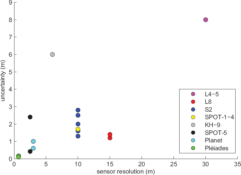
Figure 10.2. Uncertainties of displacement fields measured from optical satellite images in landslides, as a function of the sensor type. Synthesis realized from Stumpf et al. (2014, 2017, 2018), Lacroix et al. (2015, 2018, 2019, 2020), Le Bivic et al. (2017), Bontemps et al. (2018), Caporossi et al. (2018), Bradley et al. (2019), Desrues et al. (2019), Yang et al. (2019), Mazzanti et al. (2020) and Mulas et al. (2020). For a color version of this figure, see www.iste.co.uk/cavalie/images.zip
All these studies reveal a measurement accuracy highly dependent on the pixel size (from 0.15 m for Pléiades images to 8 m for L4–5 images; see Figure 10.2), as well as the time separation between images (the larger the time-separation between images, the higher the uncertainty, due to variations of the terrain properties over time), the difference between seasons and the type of vegetation cover (e.g. uncertainties are found to be lower in desertic areas than forested areas). The first satellite missions (L4–5, KH9, SPOT-1–4) had lower radiometric resolutions (the pixel radiometry was coded over less bytes) and a lower quality of sensor orientation information, leading to higher uncertainties. The uncertainties were also found to increase at the landslide borders, due to objects of different velocities being present in the same correlation window.
These uncertainties directly impact the range of landslide velocities that can be detected from optical satellite images. The ability to detect landslides is also dependent on the landslide size in relation to the satellite image pixel size. Smaller landslides can only be detected with higher resolution images. The different studies realized as of today have focused on landslides with a minimum size of 0.001 km2 with Pléiades data (Stumpf et al. 2017), 0.08 km2 with Planet data (Mazzanti et al. 2020), 0.5 km2 with L8 data (Caporossi et al. 2018) and 1 km2 with L4–5 data (Lacroix et al. 2020). To decrease the threshold of small object detection, correlators using a multi-resolution approach, such as, for instance, MicMac (Rupnik et al. 2017), are more appropriate.
Correlation techniques sometimes fail to estimate the displacement due to strong changes in the ground surface between successive images, caused, for example, by high velocities of the landslide or anthropogenic modifications. Two methods have been applied to overcome these limitations: (1) manual picking of homologous points in the satellite images (e.g. Jiang et al. 2016) and (2) use of a small temporal baseline approach to give more weight to pairs of images closer in time (Bontemps et al. 2018). Variations in the illumination (e.g. seasonal) can also result in strong displacement errors (up to 20 m in L8 images (Lacroix et al. 2019)) caused by variations of shadows in steep topographies. Post-processing based on decomposition of the displacement time series can be used to remove these seasonal artifacts (Lacroix et al. 2019).
10.2.1. Landslide detection with optical remote sensing
All detection algorithms applied to slow-moving landslides are based on the assumption that the landslide displacement direction is persistent over time. Indeed, as the landslide motion is driven by gravity forces, the direction is likely to be constant. Some authors even assume that the motion must be oriented in the direction of the slope that allows them to filter a large part of the incoherent motions (Desrues et al. 2019). The question of the scale at which the slope is calculated is therefore important, as fluctuations of the surface topography or tilted blocks due to listric faults can generate surface topography opposite to the landslide motion.
Slow-moving landslide detection has been undertaken either in pairwise processes or in time series of ground motion. In pairwise processes, the ability to detect landslides is a direct function of the uncertainty of the displacement fields produced by the correlation (Figure 10.2). Pixel-based filtering of the pairwise displacement fields can be realized, based on thresholding of geomorphological and motion indicators (slope gradient, motion orientation, motion magnitude), which makes it possible to detect slow-moving landslides, including some slow gravitational motions precursory to catastrophic failures (Lacroix et al. 2018; Desrues et al. 2019). For instance, a block of 2,000 m2 moving at 0.7 m/yr was detected as a precursor to the Chambon landslide, France, nine months before its failure (Desrues et al. 2019) using Pléiades images. Also, the use of S2 data with high-frequency acquisitions allowed us to detect that the reactivation of the Harmalière landslide in June 2016 was preceded in the three days before its failure by a movement of 1 m/day of a mass of 80,000 m2 at its headscarp (Lacroix et al. 2018).
These detections are however not automatic (they particularly rely on the choice of threshold parameters and also visual expertise). For this reason, and given the scientific and societal interest, some authors have developed semi-automatic detection methods for moving landslides based on time-series ground motion fields (Stumpf et al. 2017; Pham et al. 2018). Stumpf et al. (2017) derived a pixel-based analysis of time series of ground motion measurements that detects slow-moving landslides by thresholding an indicator of the coherence of the displacement vector directions. Using this method on high-resolution data (Pléiades images at 0.7 m resolution), Stumpf et al. (2017) detected 169 slow-moving landslides in an area of 200 km2 in the French Alps active over two years. As in all the pixel-based detection methods, filtering is required due to the pixelated look of the outputs. This algorithm has proven its efficiency and is now implemented in operational platforms (e.g. ESA-GEP). In order to decrease the number of empirical parameters in this pixel-based algorithm, another method has been proposed that models and inverts the different physical properties of the signals observed in a time series of ground motion (Pham et al. 2018). In the proposed algorithm, the landslides are modeled as monotonous displacements over time, in opposition to noises that follow a Gaussian distribution with space and to locally sparse outliers. This method, applied to a time series of 28 years of SPOT 1–7 images at 10 m resolution, allowed the authors to detect 50% more previously unknown landslides in the Colca valley in Peru.
10.2.2. Landslide characterization with optical remote sensing
The detection of slow-moving landslides from previous methods allows us to easily characterize the different parameters of a landslide, such as the extent of its active part and its activity (mean and variation of velocities with time). One important parameter for characterizing landslides is volume, as it provides an indicator of their mobility (Mitchell et al. 2019). Assessing the landslide volume is not easy using remote sensing images alone, as these images provide direct information on the surface and not on the sub-surface. Different authors have, however, developed specific methods to estimate the volume of slow-moving landslides. The 3D landslide geometry can be obtained using the balanced cross-section method (Bishop 1999) with several profiles based on the displacements extracted from displacement maps (Aryal et al. 2015). Assuming that the material has elastic properties, it is possible to invert the geometries of rectangular slip surface using inverse elastic dislocation modeling (Moro et al. 2011; Aryal et al. 2015). This assumption of elasticity is often unrealistic, especially for soft slides. Therefore, Booth et al. (2013) determined the landslide basal surface geometry based on the equation for mass conservation, using a viscous flow model with a non-Newtonian rheology. Inversion of the resulting equations using a 3D displacement field extracted from the correlation of satellite images and from the difference between successive DEMs allowed the authors to derive a thickness of up to 163 m for the large La Clapière landslide. This method was also applied later using SAR images to characterize the landslide basal geometry of a wide sets of earthflows (Handwerger et al. 2021) in California.
10.2.3. Landslide monitoring with optical remote sensing
Landslide monitoring is based on the generation of displacement time series. The constant availability of satellite optical data since the 1970s, as well as the increased frequency of image acquisitions in recent years, have enabled scientists to monitor a wide variety of landslide activities, from transient motions at sub-weekly scales to long-term evolution over decadal scales. High-frequency S2 and L8 satellites have enabled the detection of daily variations of landslide velocities prior to a major landslide reactivation (Lacroix et al. 2018). Sudden acceleration of landslides was also observed thanks to S2 and L8 satellites in a Peruvian desert, with velocities reaching 1 m/day followed by a constant deceleration over three months until they reached quiescence or a steady state (Lacroix et al. 2019, 2020) (Figure 10.3). These motions were related to the supply of new material on the landslide body coming from regression of the headscarp. In seismically active regions, the time series of landslide displacements can also reveal the earthquake forcing the slow-moving landslide kinematics, as observed in the Colca region in Peru (Lacroix et al. 2015).
Over seasonal time-scales, landslides may display sinusoidal motion related to groundwater effects, as observed in the Barcelonette area, France (Stumpf et al. 2017). These seasonal signals in optical images must however be interpreted with caution. Indeed, seasonal differences of illumination can create an artifact of displacement, the magnitude of which is a function of the slope gradient and orientation (Lacroix et al. 2019). These artifacts can reach up to 20 m in steep slopes on L8 images and must therefore be corrected. To remove these artifacts, several options exist: only using images taken from the same season, removing a seasonal sinusoid from the data for the phase and amplitudes calculated over stable areas (Lacroix et al. 2019) or masking the shadows before the correlation step.
In the longer term, image-correlation time series have been applied in several case studies, highlighting the complex combination of different forcings (earthquake, rainfall) in the landslide kinematics of the Maca valley, Peru, over 28 years (Bontemps et al. 2018), for instance, or irrigation impacts on the landslides from the desertic area of the Siguas and Vitor valleys, Peru, over 40 years (Lacroix et al. 2020).
These different time-scales highlight different physical processes and forcings acting on landslides (Lacroix et al. 2020). The monitoring of landslides from optical images is therefore of significant interest for the study of the mechanics of landslides and the response to external forcings. Satellite monitoring can also be complemented with in situ measurements of different physical parameters to decipher the complex mechanics of landslides, although the latter depend on accessibility and feasibility.
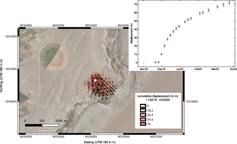
Figure 10.3. Displacement field and time series of displacement in the Pachaqui landslide (Peru), as estimated using Sentinel-2 data (see Lacroix et al. (2020)). The time series shows the sudden acceleration of the landslide in December 2019, following a retrogression of the landslide headscarp and the subsequent material supply to the landslide body. For a color version of this figure, see www.iste.co.uk/cavalie/images.zip
10.3. Offset tracking of SAR images applied to landslides
The correlation of SAR amplitude images, also known as offset tracking (see Chapter 3), has recently been applied in landslide investigations, and it efficiently complements the correlation of optical images in areas where frequent cloud cover prevents their use (Dille et al. 2021). This technique can be applied to landslides when patterns, due to persistent features or to correlated speckle, exist and are visible in the diachronic SAR pairs. This technique leads to the retrieval of displacement in the range and azimuth directions of the radar. Three-dimensional displacement fields can be obtained for landslides when both ascending and descending tracks are processed for the same area (e.g. Raucoules et al. 2013). Pre-processing of SAR images is necessary in order to obtain a multi-temporal stack coregistered to a reference SAR image (using a digital elevation model) before measuring the sub-pixel offsets from one image to another (to eliminate the topography and orbital offsets from the results). Large correlation windows are often required, as the texture patterns of the SAR amplitude are usually of larger wavelengths than the texture of objects in optical images where many ground features can be detected. Also, due to the different resolutions in the range and azimuth directions, different window sizes are sometimes chosen along these two dimensions to try to decrease the real ground pixel size in one dimension (Sun et al. 2017). The correlation window sizes used in past studies range between 32 and 64 pixels in the less-defined direction. Smaller window sizes are generally used for high-resolution SAR satellites (TerraSAR-X (TSX) (Sun and Muller 2016; Sun et al. 2017), COSMO SkyMed (CSK) (Raspini et al. 2015)) than for lower-resolution satellites, such as Sentinel-1 (S1) (Manconi et al. 2018). Large window sizes restrict the application of offset tracking techniques to only large landslides and prevent the detection of small objects.
This size limitation led most previous landslide studies to focus on high-resolution SAR data, such as TSX (Raucoules et al. 2013; Singleton et al. 2014; Sun and Muller 2016; Sun et al. 2017), CSK (Raspini et al. 2015; Caporossi et al. 2018) or ALOS-2 images (Jia et al. 2020). Other studies have, however, focused on the use of lower-resolution SAR images, such as S1 (Manconi et al. 2018; Li et al. 2020), with about 14 m pixel spacing in azimuth and 3 m in range. The latter images have the advantages of being open access and of having a high revisit rate, increasing the potential for investigation of the time evolution of the landslide kinematics. Few attempts have been made to create time series of landslide displacement with these data due to the low landslide detection ability of these middle-resolution satellites. Li et al. (2020) used the full archives of S1 and ALOS for the large Baige landslide in China, covering 12 years, to estimate the precursory motion of this landslide before its failure. Time series of landslide displacements are, however, more common using TSX (Raucoules et al. 2013; Singleton et al. 2014) or CSK images (Caporossi et al. 2018), but their cost makes their global and systematic application unfeasible.
The uncertainty of the method has barely been quantified for landslides. Some authors estimated the uncertainties by calculating the dispersion (STD) of the displacement field in stable areas and found about 0.1 m of uncertaintiy for ALOS data (Jia et al. 2020). Raucoules et al. (2013) compared the results from TSX image correlation with GNSS-2 for the La Valette landslide (France) and found 12 and 8 cm uncertainties in the horizontal and vertical motions, respectively, corresponding to about 1/10th of the pixel size. Singleton et al. (2014) compared the offset tracking results with 17 corner reflectors installed on a landslide in China and found RMS errors of 4 cm in range and 7 cm in azimuth using TSX stripmap data and 1 cm in range and 6 cm in azimuth for TSX spotlight data (0.8 x 0.25 m resolution images).
A limitation of the offset tracking techniques for landslides is the orientation of the landslide with respect to the radar. In order to avoid layover, the more favorably oriented landslides are those that face away from the satellite (to be covered by a sufficiently large number of radar pixels, at least several times the correlation window size) without being too steep (to avoid shadowing), or those that face towards the satellite but on gentle slopes (Figure 10.4). Furthermore, the pixels of radar images are often not squared (for instance, about 3 x 14 m in the range and azimuth directions for S1 images), which makes the accuracy of the algorithm different in range and in azimuth. This reduces the applicability of the algorithm for a specific dataset or any given landslide. All these limitations have restricted the application of this method to a few cases, despite its great potential for time-series generation with any cloud cover conditions.
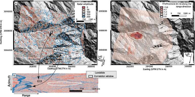
Figure 10.4. Sentinel-1 SAR amplitude image shown projected onto a DEM (A) and in radar geometry (B). The white line shows the contour of a slow-moving landslide oriented along the range direction of the satellite. The correlation of two SAR images (C) shows a landslide displacement of –13 m along the line of sight of the satellite, that is, flowing away from the satellite. The black frames on subplots A and B are indicative of the correlation windows used at two locations and their corresponding real sizes in geographical coordinates (A). For a color version of this figure, see www.iste.co.uk/cavalie/images.zip
10.4. InSAR for landslide studies
Since the first launches of civil SAR satellites in the 1990s (ERS, JERS, Radarsat), InSAR techniques have been applied to detect and monitor landslides (e.g. Carnec et al. 1996). InSAR is better suited to the study of very slow- to slow-moving landslides (Colesanti and Wasowski 2006; Handwerger et al. 2013; Wasowski and Bovenga 2014) with average velocities of mm/yr or cm/yr, using traditional C-band or X-band radars. However, longer wavelength (L-band and upcoming S-band) and/or high revisit rates might allow for the detection of faster displacements. The choice of the wavelength depends not only on the expected landslide velocity but also on the land cover of the area of interest. For instance, X-band signals are well suited to studying urban environments, where buildings and infrastructure offer radiometrically stable scatterers, with limited decorrelation over time. Individual, large infrastructures also benefit from monitoring with X-band due to its high sensitivity to smaller displacements and the high resolution of satellites such as the CSK and the TSX constellations (1–3 m). L-band radar is best suited for vegetated terrains, as the longer wavelength (~24 cm) is less sensitive to changes associated with growth in comparison to X- and C-band sensors (Schlögel et al. 2015; Nishiguchi et al. 2017). For example, Dini et al. (2019b), who carried out a study based on single interferogram analysis both in C- and L-band over a large area in Bhutan, reported that 92% of the objects detected were through L-band interferograms generated with ALOS-1 images.
10.4.1. Standard versus multi-temporal InSAR analyses
Standard and more advanced multi-temporal methods for the identification, classification, characterization, quantification and monitoring of displacements caused by geological and geomorphological processes of different natures in mountainous terrain are extensively documented in the literature. Standard methods generally rely on the generation and analysis of single interferograms, as snapshots of the deformation between two successive acquisitions. Examples of this application are available for the detection and inventorying of slope instabilities (Delaloye et al. 2007, e.g.), for the interpretation and quantification of surface displacements of different origins (e.g. Massonnet and Feigl 1998; Colesanti and Wasowski 2006; Cignetti et al. 2016) and for the classification of the geomorphological processes leading to the observed displacements (e.g. Dini et al. 2019b). Although a single interferogram is, as mentioned above, a mere snapshot of displacement occurring between two acquisitions, a detailed and in-depth analysis of a large number of interferograms over an area of interest can be quite revealing and, in fact, complementary to multi-temporal analyses in landslide applications (Figure 10.5). The analysis of interferograms of different temporal baselines can, for instance, reveal different phases of landslide activity through time.
Multi-temporal methods are based on the use of several interferograms for the extraction of velocity maps and time series. Retrieving a time-series of displacements enables us to evaluate the evolution of the kinematics underpinning the observed process. However, this is not the only advantage of multi-temporal analyses. The generation of time series can also mitigate unwanted effects (e.g. atmospheric artifacts) that may overprint the displacement signal and thus overcomes some of the limitations of standard differential SAR interferometry (Wasowski and Bovenga 2014). There are different types of approaches for InSAR time-series generation (see Chapter 5). Methods that take advantage of dominant single-point scatterers, such as the permanent scatterer approach (PS-InSAR) (Ferretti et al. 2001), yield good results in urbanized environments or over a large infrastructure. Other methods take advantage of the presence of distributed scatterers within each pixel. Among these, the small baseline subset (SBAS) approach (Berardino et al. 2002) is widely used. Distributed scatterers are those that characterize many natural land cover types, where no dominant contribution from individual features, such as debris or loose soil, exists. As opposed to urban environments, permanent scatterers are often fewer in natural landscapes, where they are generally provided by bare rock outcrops. In order to increase the number of exploitable scatterers for landslides, various methods that combine the advantages of the two previous groups have been developed, such as SqueeSAR (e.g. Ferretti et al. 2011; Intrieri et al. 2018) or StaMPS PS-InSAR (Kiseleva et al. 2014). The accuracy that can be obtained is in general of the order of 1–2 mm/yr for annual velocities and 5–10 mm/yr for cumulative displacements (Catani et al. 2014; Wasowski and Bovenga 2014).
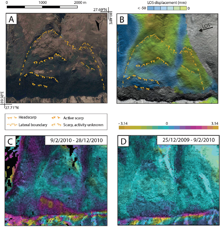
Figure 10.5. A) Large, slow-moving landslide in NW Bhutan with mapped geomorphological features (modified from Dini et al. (2019b)); B) ALOS-1 cumulative displacements obtained with SBAS between February 2007 and February 2011 (modified from Dini et al. (2019a)); C and D) wrapped interferograms obtained with ALOS-1 data. For a color version of this figure, see www.iste.co.uk/cavalie/images.zip
10.4.2. Limitations in the use of SAR interferometry for landslide applications
Despite its great potential for landslide studies, InSAR suffers from limitations that need to be carefully evaluated when conceiving new research as well as during the interpretation of results. Some of the limitations are specific to landslide applications. Landslides often occur in environmental settings that are difficult for InSAR applications; these include natural slopes on which individual, dominant scatterers are rare, dense vegetation and alpine climates entailing extensive snow cover. Land cover types such as those mentioned are unfavorable from the point of view of interferometric stability as they lead to low coherence over time (e.g. Cignetti et al. 2016). This, in turn, is associated with a scarcity of points for which displacement measurements can be reliably retrieved (Wasowski and Bovenga 2014), compromising the robustness and interpretation of the results.
Moreover, when working with landslides, it is not unusual to deal with areas characterized by high topographic gradients. Rough topography leads to geometrical distortions that can severely hinder the retrieval of interferometric information. This problem can, in some cases, be overcome with the use of ascending and descending geometries, but this is subject to acquisition availability and requires case-by-case evaluation. Moreover, satellites that carry SAR sensors follow orbits that are near-polar. This leads to a greater visibility of slope movements that are oriented east–west; thus, landslides that face north or south are difficult to image with InSAR as movements are only detected in the line of sight of the sensor. Thus, displacements occurring in the north–south direction cannot be resolved without making important assumptions (Samsonov et al. 2020).
In areas of rough topography, strong effects associated with the stratified atmosphere are often observed, affecting the entire scene. The phase changes associated with these effects are of long wavelengths and do not necessarily impair the simple detection of landslides, given the small size of the investigated area, but the retrieval of reliable time series and of reasonable average velocities can be hindered by the overprint of the atmospheric delay (e.g. Dini et al. 2019a) and can even cause the stable point chosen to be affected by seasonal oscillations.
An important limitation is related to an effect that is referred to as phase aliasing. The phase information is measured modulo 2π (see Chapter 6). Thus, it is not possible to unambiguously detect displacements that exceed in general a quarter of the wavelength between two successive acquisitions and two adjacent pixels (e.g. Wasowski and Bovenga 2014; Manconi 2021). When the displacement gradient exceeds this value, aliasing occurs and information on the displacement is not retrieved or severely underestimated. What this threshold corresponds to exactly is difficult to establish as it does not only depend on the displacement in the time interval between two acquisitions but also on the area affected by the displacements.
10.4.3. Landslide detection with InSAR
Many studies have now shown the interest of InSAR for detection and inventorying of slope movements. Delaloye et al. (2007), for example, used ERS data to generate a relatively small number of interferograms in which a large number of mass movements in the periglacial environment of the Swiss Alps were identified. Dini et al. (2019b) used a similar approach and visually inspected a large number of interferograms computed with ENVISAT (C-band) and ALOS-1 (L-band) SAR data. This allowed for the identification of a large number of previously unknown instabilities in the Himalayas of northwestern Bhutan. Moreover, Dini et al. (2019a) used the same dataset to generate, with the SBAS approach, average velocity and cumulative displacements maps on which more patterns associated with slope instabilities could be detected and inventoried, highlighting the complementary aspect of individual interferogram analysis and that of large-scale average velocity for landslide detection. The example in Figure 10.5 shows that, on the one hand, wrapped single interferograms may not allow the detection of slow displacement rates at shorter temporal baselines. The 46-day interferogram in Figure 10.5(D) shows only a weak signal at the bottom of the slope, likely due to a phase of deceleration during the dry season and to the short temporal baseline. The 10-month interferogram in Figure 10.5(C) shows significant activity in the lower part of the slope, but not in the upper half, hence some structures visible in the optical images and in the DEM would appear to be inactive through analysis of the interferograms. On the other hand, the difficulties that arise, for instance, the loss of coherence due to unfavorable land cover or during phase unwrapping related to aliasing, can cause loss of scatterers over large areas in multi-temporal processing approaches. For instance, the cumulative displacements obtained with a multi-temporal approach in Figure 10.5(B) show no information for the lower part of the slope, likely due to temporal decorrelation (presence of vegetation, fast displacements), while activity can be observed in the upper part of the slope where displacements are too subtle to be seen in individual interferograms. The use of PS-InSAR results at the regional scale, and in combination with ancillary data, has been attempted for the interpretation of velocity ranges, aiming at improving existing landslide inventories (e.g. Rosi et al. 2018).
The availability of InSAR-based inventories thus requires careful interpretation of the possible processes causing the detected displacements. Geomorphological analyses carried out visually with optical images are again commonly associated with this task. This does not only require expertise in the recognition of geomorphological features as descriptors of the investigated mass movements but also a sound knowledge of the main pitfalls and possible artifacts related to InSAR results. For example, Cignetti et al. (2016) performed a regional multi-temporal analysis based on the SBAS approach and compared the average velocity results with existing large, slow-moving landslide and rock glacier inventories in order to steer the interpretation of the InSAR results.
10.4.4. Landslide characterization with InSAR
At the site scale, some authors have demonstrated methods that combine the analysis of the spatial distribution of both surface geomorphological features and SAR phase values (Schlögel et al. 2015). Morphological features such as scarps, fractures, lobes and gullies are mapped on optical images or DEMs and are then used to guide the interpretation of wrapped and unwrapped interferograms. Although this type of methodology requires detailed geomorphological mapping and geophysical knowledge of the landslide for the interpretation of the InSAR deformation fields, it provides a basis for the investigation landslide mechanisms for rotational, translational and complex movements. At the regional scale, recent studies have shown the potential of InSAR in combination with geomorphological analyses for the association of the displacements obtained with specific landforms and with the geological material types involved, in order to give an interpretation to the processes (e.g. Dini et al. 2019a). The authors of these studies have used different approaches in order to unravel reversible seasonal and irreversible gravitational displacements, including those occurring in periglacial environments. They have also demonstrated the use of ascending and descending geometries in the decomposition between vertical and east–west components in obtaining 2D InSAR displacements (Rouyet et al. 2019; Daout et al. 2020). Moreover, just the analysis of the aspect dependence of the signal in the two acquisition geometries can reveal whether the largest component of the displacement is vertical or horizontal. With this type of analysis, insights can be gained regarding the dominant processes occurring in understudied slopes, as well as in the interannual variability of freeze–thaw cycles, in long-term permafrost variations and in groundwater table-induced displacements below the permafrost region. Methods involving the use of PS-InSAR and SqueeSAR data, as well as single interferograms, have been developed to characterize the kinematics of large, slow-moving landslides in the Italian Alps (Crippa et al. 2021). Such methods focus on the classification of observed average velocities, as well as on the presence of nested sectors within a landslide and the style of activity. This type of analyses is able to reveal, even at the regional scale, composite slope instabilities with nested sectors that might undergo different evolutionary trends towards failure.
10.4.5. Landslide monitoring with InSAR
InSAR-derived time-series can be used to evaluate external forcing on landslides of natural or anthropogenic origin. Handwerger et al. (2013) were able to show the annual velocity variations of slow-moving landslides in northern California with ALOS data and the delayed response of landslide accelerations to rainfall. The accuracy and coverage obtained with L-band SAR data made it possible to unravel the dependency between landslide kinematics and minor pore pressure changes. Coseismic reactivations of large landslides in Italy were imaged with the generation of interferograms, and the displacements observed were used to validate the displacements obtained through modeling of the rupture surface and the instantaneous deformation postulated (Moro et al. 2011). The availability of multiple sensors enabled the generation of long time-series (≈20 yrs) and thus established causal effects between landslide velocities and triggers. For example, Strozzi et al. (2010) used InSAR in combination with other data to show the long-term evolution of a landslide in the Swiss Alps that was activated as a consequence of glacier retreat and presented acceleration phases related to snow melt and intense rainfall events. The quantification of displacements for very slow landslides using multi-temporal and multi-sensor InSAR analyses has also been shown to reveal evidence of recent activity in response to natural and anthropogenic factors (e.g. fluvial erosion, excavation, overloading, enhanced infiltration) (Herrera et al. 2013). Furthermore, excavations and stabilization measures have effects on natural slopes and the quantification of velocities through InSAR time-series has been shown to be a valuable tool to enhance the understanding of the interactions (Dini et al. 2020).
In the context of hazard assessment, landslide damage maps can be produced based on thresholds of deformation calculated over InSAR-derived LOS velocities or its projection along the line of maximum gradient of a landslide (e.g. Herrera et al. 2013; Barra et al. 2017; Solari et al. 2019). This type of analysis can be used with predictive aims, if thresholds are to be set above which damage might be expected. Barra et al. (2017) and Solari et al. (2019) used multi-temporal InSAR analyses based on PS-InSAR and SqueeSAR to retrieve “hot spots” of deformation over large regions. The aim was identifying and monitoring, through regular updates of the time series, areas characterized by active deformation. As the spatio-temporal noise of the InSAR results and velocity maps can contain a large number of points, this type of methodology strives to improve the readability of the results to be used in an operational context. This type of work is essential to bridge the gap that exists between retrieving the interferometric information and feeding this data into hazard and risk assessments in an easily readable, reliable and quantitative way.
The launch of satellites with high revisit rates (up to six days revisit time) is now allowing scientists to begin to consider the viability of closely monitoring displacements occurring on slopes and landslide velocity through time, as opposed to carrying out retrospective studies using archived data. This is appealing because effective monitoring can be used to establish clear triggering mechanisms and potentially provide alerts on thresholds. Timely monitoring would make it possible to apply inverse velocity methods with predictive abilities to InSAR velocity data. This possibility is still limited by unfavorable combinations of wavelengths and revisit rates with regard to landslide velocity, with phase aliasing potentially causing severe underestimations of the displacement rates which would prevent accurate failure forecasts (e.g. Manconi 2021). However, more authors are beginning to point towards the possibility of establishing regional-scale early-warning systems based on the continuous processing of S1 data due to its regularity of acquisition. Updated displacement time-series can be used to systematically feed landslide failure forecast models that require the timely identification of accelerations (Raspini et al. 2018). Recently, some notable case studies have been analyzed by means of back-analyses with InSAR multi-temporal techniques (e.g. Intrieri et al. 2018), in the attempt to detect precursory signals of failure and to establish whether such information could have been obtained pre-emptively and converted into an early warning. Although these studies are carried out post-failure, thus with plenty of available time for processing and analysis and with previous knowledge of the studied landslide, the findings are encouraging and seem to indicate that the better temporal resolution of S1 and the future launch of L-band satellites with high revisit rates (NISAR) might allow scientists to better analyze the evolution of a landslide as it unfolds, implying that some viable lead time for alerts might be reached in the future with this technique.
10.5. Conclusion
Satellite images have proven their efficiency in detecting, characterizing and monitoring slow-moving landslides with velocities from mm/yr to m/day, often situated in remote and/or steep areas. The specificities of landslides (small size, rough topography, high variability of velocity through time, variable terrain cover such as vegetation or snow) make the use of a combination of various sensors onboard satellites key for all these applications.
The availability of an increasingly large pool of sensors and the development of new methodologies allows for expert combination of different types of satellite data and methods. This represents a key factor in many landslide studies based on remote sensing, maximizing the potential for displacement retrieval and making use of the advantages and the complementarity of different techniques.
The significant time depth now covered by satellite images (up to 60 years) allows for the generation of long time-series of slow-moving landslide displacements over wide areas. This is of specific interest for the study of landslide processes in a changing world, where both climate change and anthropogenic stress on the natural environment are prominent. The study of these two forcings on landslide processes can therefore start to be inferred thoroughly.
The launch of high-resolution satellites and high-frequency satellites provides new opportunities to better study the physical processes of landslides in relation to their forcing factors, to map them more accurately and to estimate the related hazard. In particular, some back-analyses of catastrophic landslides have shown the existence of coherent motion before failure that can be measured with both SAR and optical images. The combination of different high-frequency satellites will certainly be of interest for such objectives. This rather operational prospective must not hide the large challenges research still has to face, related, for instance, to big data processing, transient motion detection abilities over large areas and integration of different sources of data.
10.6. References
Aryal, A., Brooks, B.A., Reid, M.E. (2015). Landslide subsurface slip geometry inferred from 3-D surface displacement fields. Geophysical Research Letters, 42(5), 1411–1417.
Barra, A., Solari, L., Béjar-Pizarro, M., Monserrat, O., Bianchini, S., Herrera, G., Crosetto, M., Sarro, R., González-Alonso, E., Mateos, R.M., Ligüerzana, S., López, C., Moretti, S. (2017). A methodology to detect and update active deformation areas based on Sentinel-1 SAR images. Remote Sensing, 9(10), 1002.
Berardino, P., Fornaro, G., Lanari, R., Sansosti, E. (2002). A new algorithm for surface deformation monitoring based on small baseline differential SAR interferograms. IEEE Transactions on Geoscience and Remote Sensing, 40(11), 2375–2383.
Bishop, K.M. (1999). Determination of translational landslide slip surface depth using balanced cross sections. Environmental and Engineering Geoscience, 2, 147–156.
Bontemps, N., Lacroix, P., Doin, M.-P. (2018). Inversion of deformation fields time-series from optical images, and application to the long term kinematics of slow-moving landslides in Peru. Remote Sensing of Environment, 210, 144–158.
Booth, A.M., Lamb, M.P., Avouac, J.-P., Delacourt, C. (2013). Landslide velocity, thickness, and rheology from remote sensing: La Clapière landslide, France. Geophysical Research Letters, 40(16), 4299–4304.
Bradley, K., Mallick, R., Andikagumi, H., Hubbard, J., Meilianda, E., Switzer, A., Du, N., Brocard, G., Alfian, D., Benazir, B. et al. (2019). Earthquake-triggered 2018 Palu Valley landslides enabled by wet rice cultivation. Nature Geoscience, 12(11), 935–939.
Caporossi, P., Mazzanti, P., Bozzano, F. (2018). Digital image correlation (DIC) analysis of the 3 December 2013 Montescaglioso Landslide (Basilicata, Southern Italy): Results from a multi-dataset investigation. ISPRS International Journal of Geo-Information, 7(9), 372.
Carnec, C., Massonnet, D., King, C. (1996). Two examples of the use of SAR interferometry on displacement fields of small spatial extent. Geophysical Research Letters, 23(24), 3579–3582.
Catani, F., Canuti, P., Casagli, N. (2014). The use of radar interferometry in landslide monitoring. In Landslides in Cold Regions in the Context of Climate Change, Shan, W., Guo, Y., Wang, F., Marui, H., Strom, A. (eds). Springer, Cham.
Cignetti, M., Manconi, A., Manunta, M., Giordan, D., De Luca, C., Allasia, P., Ardizzone, F. (2016). Taking advantage of the ESA G-POD service to study ground deformation processes in high mountain areas: A Valle D’Aosta case study, Northern Italy. Remote Sensing, 8(10), 852.
Colesanti, C. and Wasowski, J. (2006). Investigating landslides with space-borne synthetic aperture radar (SAR) interferometry. Engineering Geology, 88(3–4), 173–199.
Crippa, C., Valbuzzi, E., Frattini, P., Crosta, G.B., Spreafico, M.C., Agliardi, F. (2021). Semi-automated regional classification of the style of activity of slow rock-slope deformations using PS InSAR and SqueeSAR velocity data. Landslides, 1–19.
Daout, S., Dini, B., Haeberli, W., Doin, M.-P., Parsons, B. (2020). Ice loss in the northeastern Tibetan Plateau permafrost as seen by 16 yr of ESA SAR missions. Earth and Planetary Science Letters, 545, 116404.
Delacourt, C., Allemand, P., Casson, B., Vadon, H. (2004). Velocity field of the “La Clapière” landslide measured by the correlation of aerial and QuickBird satellite images. Geophysical Research Letters, 31(15).
Delaloye, R., Lambiel, C., Lugon, R., Raetzo, H., Strozzi, T. (2007). Typical ERS InSAR signature of slope movements in a periglacial mountain environment (Swiss Alps). Envisat Symposium, Montreux, Switzerland, 23–27 April.
Desrues, M., Lacroix, P., Brenguier, O. (2019). Satellite pre-failure detection and in situ monitoring of the landslide of the Tunnel du Chambon, French Alps. Geosciences, 9(7), 313.
Dille, A., Kervyn, F., Handwerger, A.L., d’Oreye, N., Derauw, D., Bibentyo, T.M., Samsonov, S., Malet, J.-P., Kervyn, M., Dewitte, O. (2021). When image correlation is needed: Unravelling the complex dynamics of a slow-moving landslide in the tropics with dense radar and optical time series. Remote Sensing of Environment, 258, 112402.
Dini, B., Daout, S., Manconi, A., Loew, S. (2019a). Classification of slope processes based on multitemporal DInSAR analyses in the Himalaya of NW Bhutan. Remote Sensing of Environment, 233, 111408.
Dini, B., Manconi, A., Loew, S. (2019b). Investigation of slope instabilities in NW Bhutan as derived from systematic DInSAR analyses. Engineering Geology, 259, 105111.
Dini, B., Manconi, A., Loew, S., Chophel, J. (2020). The Punatsangchhu-I dam landslide illuminated by InSAR multitemporal analyses. Scientific Reports, 10(1), 1–10.
Ferretti, A., Prati, C., Rocca, F. (2001). Permanent scatterers in SAR interferometry. IEEE Transactions on Geoscience and Remote Sensing, 39(1), 8–20.
Ferretti, A., Fumagalli, A., Novali, F., Prati, C., Rocca, F., Rucci, A. (2011). A new algorithm for processing interferometric data-stacks: SqueeSAR. IEEE Transactions on Geoscience and Remote Sensing, 49(9), 3460–3470.
Froude, M.J. and Petley, D.N. (2018). Global fatal landslide occurrence from 2004 to 2016. Natural Hazards and Earth System Sciences, 18(8), 2161–2181.
Guzzetti, F., Mondini, A.C., Cardinali, M., Fiorucci, F., Santangelo, M., Chang, K.-T. (2012). Landslide inventory maps: New tools for an old problem. Earth-Science Reviews, 112(1–2), 42–66.
Handwerger, A.L., Roering, J.J., Schmidt, D.A. (2013). Controls on the seasonal deformation of slow-moving landslides. Earth and Planetary Science Letters, 377, 239–247.
Handwerger, A.L., Booth, A.M., Huang, M.-H., Fielding, E.J. (2021). Inferring the subsurface geometry and strength of slow-moving landslides using 3-D velocity measurements from the NASA/JPL UAVSAR. Journal of Geophysical Research: Earth Surface, 126(3), e2020JF005898.
Herrera, G., Gutiérrez, F., García-Davalillo, J., Guerrero, J., Notti, D., Galve, J., Fernández-Merodo, J., Cooksley, G. (2013). Multi-sensor advanced DInSAR monitoring of very slow landslides: The Tena Valley case study (Central Spanish Pyrenees). Remote Sensing of Environment, 128, 31–43.
Hungr, O., Leroueil, S., Picarelli, L. (2014). The Varnes classification of landslide types, an update. Landslides, 11(2), 167–194.
Intrieri, E., Raspini, F., Fumagalli, A., Lu, P., Del Conte, S., Farina, P., Allievi, J., Ferretti, A., Casagli, N. (2018). The Maoxian landslide as seen from space: Detecting precursors of failure with Sentinel-1 data. Landslides, 15(1), 123–133.
Jia, H., Wang, Y., Ge, D., Deng, Y., Wang, R. (2020). Improved offset tracking for predisaster deformation monitoring of the 2018 Jinsha River landslide (Tibet, China). Remote Sensing of Environment, 247, 111899.
Jiang, S., Wen, B.-P., Zhao, C., Li, R.-D., Li, Z.-H. (2016). Kinematics of a giant slow-moving landslide in northwest China: Constraints from high resolution remote sensing imagery and GPS monitoring. Journal of Asian Earth Sciences, 123, 34–46.
Kiseleva, E., Mikhailov, V., Smolyaninova, E., Dmitriev, P., Golubev, V., Timoshkina, E., Hooper, A., Samiei-Esfahany, S., Hanssen, R. (2014). PS-InSAR monitoring of landslide activity in the Black Sea coast of the Caucasus. Procedia Technology, 16, 404–413.
Lacroix, P., Berthier, E., Maquerhua, E.T. (2015). Earthquake-driven acceleration of slow-moving landslides in the Colca Valley, Peru, detected from Pléiades images. Remote Sensing of Environment, 165, 148–158.
Lacroix, P., Bièvre, G., Pathier, E., Kniess, U., Jongmans, D. (2018). Use of Sentinel-2 images for the detection of precursory motions before landslide failures. Remote Sensing of Environment, 215, 507–516.
Lacroix, P., Araujo, G., Hollingsworth, J., Taipe, E. (2019). Self entrainment motion of a slow-moving landslide inferred from Landsat-8 time-series. Journal of Geophysical Research – Earth Surface, 124, 1201–1216.
Lacroix, P., Dehecq, A., Taipe, E. (2020a). Irrigation-triggered landslides in a Peruvian desert caused by modern intensive farming. Nature Geoscience, 13(1), 56–60.
Lacroix, P., Handwerger, A.L., Bièvre, G. (2020b). Life and death of slow-moving landslides. Nature Reviews Earth & Environment, 1(8), 404–419.
Le Bivic, R., Allemand, P., Quiquerez, A., Delacourt, C. (2017). Potential and limitation of SPOT-5 ortho-image correlation to investigate the cinematics of landslides: The example of “Mare à Poule d’Eau” (Réunion, France). Remote Sensing, 9(2), 106.
Li, M., Zhang, L., Ding, C., Li, W., Luo, H., Liao, M., Xu, Q. (2020). Retrieval of historical surface displacements of the Baige landslide from time-series SAR observations for retrospective analysis of the collapse event. Remote Sensing of Environment, 240, 111695.
Manconi, A. (2021). How phase aliasing limits systematic space-borne DInSAR monitoring and failure forecast of alpine landslides. Engineering Geology, 287, 106094.
Manconi, A., Kourkouli, P., Caduff, R., Strozzi, T., Loew, S. (2018). Monitoring surface deformation over a failing rock slope with the ESA sentinels: Insights from Moosfluh instability, Swiss Alps. Remote Sensing, 10(5), 672.
Massonnet, D. and Feigl, K.L. (1998). Radar interferometry and its application to changes in the earth’s surface. Reviews of Geophysics, 36(4), 441–500.
Mazzanti, P., Caporossi, P., Muzi, R. (2020). Sliding time master digital image correlation analyses of CubeSat images for landslide monitoring: The Rattlesnake Hills landslide (USA). Remote Sensing, 12(4), 592.
Mitchell, A., McDougall, S., Nolde, N., Brideau, M.-A., Whittall, J., Aaron, J. (2019). Rock avalanche runout prediction using stochastic analysis of a regional dataset. Landslides, 17, 777–792.
Moro, M., Chini, M., Saroli, M., Atzori, S., Stramondo, S., Salvi, S. (2011). Analysis of large, seismically induced, gravitational deformations imaged by high-resolution COSMO-SkyMed synthetic aperture radar. Geology, 39(6), 527–530.
Mulas, M., Ciccarese, G., Truffelli, G., Corsini, A. (2020). Integration of digital image correlation of Sentinel-2 data and continuous GNSS for long-term slope movements monitoring in moderately rapid landslides. Remote Sensing, 12(16), 2605.
Nishiguchi, T., Tsuchiya, S., Imaizumi, F. (2017). Detection and accuracy of landslide movement by InSAR analysis using PALSAR-2 data. Landslides, 14(4), 1483–1490.
Pham, M.Q., Lacroix, P., Doin, M.P. (2018). Sparsity optimization method for slow-moving landslides detection in satellite image time-series. IEEE Transactions on Geoscience and Remote Sensing, 57(4), 2133–2144.
Raspini, F., Ciampalini, A., Del Conte, S., Lombardi, L., Nocentini, M., Gigli, G., Ferretti, A., Casagli, N. (2015). Exploitation of amplitude and phase of satellite SAR images for landslide mapping: The case of Montescaglioso (South Italy). Remote Sensing, 7(11), 14576–14596.
Raspini, F., Bianchini, S., Ciampalini, A., Del Soldato, M., Solari, L., Novali, F., Del Conte, S., Rucci, A., Ferretti, A., Casagli, N. (2018). Continuous, semi-automatic monitoring of ground deformation using Sentinel-1 satellites. Scientific Reports, 8(1), 1–11.
Raucoules, D., de Michele, M., Malet, J.-P., Ulrich, P. (2013). Time-variable 3D ground displacements from high-resolution synthetic aperture radar (SAR). Application to La Valette landslide (South French Alps). Remote Sensing of Environment, 139, 198–204.
Rosi, A., Tofani, V., Tanteri, L., Stefanelli, C.T., Agostini, A., Catani, F., Casagli, N. (2018). The new landslide inventory of Tuscany (Italy) updated with PS-InSAR: Geomorphological features and landslide distribution. Landslides, 15(1), 5–19.
Rouyet, L., Lauknes, T.R., Christiansen, H.H., Strand, S.M., Larsen, Y. (2019). Seasonal dynamics of a permafrost landscape, Adventdalen, Svalbard, investigated by InSAR. Remote Sensing of Environment, 231, 111236.
Rupnik, E., Daakir, M., Deseilligny, M.P. (2017). MicMac – A free, open-source solution for photogrammetry. Open Geospatial Data, Software and Standards, 2(1), 1–9.
Samsonov, S., Dille, A., Dewitte, O., Kervyn, F., d’Oreye, N. (2020). Satellite interferometry for mapping surface deformation time series in one, two and three dimensions: A new method illustrated on a slow-moving landslide. Engineering Geology, 266, 105471.
Schlögel, R., Doubre, C., Malet, J.-P., Masson, F. (2015). Landslide deformation monitoring with ALOS/PALSAR imagery: A D-InSAR geomorphological interpretation method. Geomorphology, 231, 314–330.
Schulz, W.H., McKenna, J.P., Kibler, J.D., Biavati, G. (2009). Relations between hydrology and velocity of a continuously moving landslide – Evidence of pore-pressure feedback regulating landslide motion? Landslides, 6(3), 181–190.
Singleton, A., Li, Z., Hoey, T., Muller, J.-P. (2014). Evaluating sub-pixel offset techniques as an alternative to D-InSAR for monitoring episodic landslide movements in vegetated terrain. Remote Sensing of Environment, 147, 133–144.
Solari, L., Del Soldato, M., Montalti, R., Bianchini, S., Raspini, F., Thuegaz, P., Bertolo, D., Tofani, V., Casagli, N. (2019). A Sentinel-1 based hot-spot analysis: Landslide mapping in north-western Italy. International Journal of Remote Sensing, 40(20), 7898–7921.
Strozzi, T., Delaloye, R., Kääb, A., Ambrosi, C., Perruchoud, E., Wegmüller, U. (2010). Combined observations of rock mass movements using satellite SAR interferometry, differential GPS, airborne digital photogrammetry, and airborne photography interpretation. Journal of Geophysical Research: Earth Surface, 115(F1).
Stumpf, A., Malet, J.P., Allemand, P., Ulrich, P. (2014). Surface reconstruction and landslide displacement measurements with Pléiades satellite images. ISPRS Journal of Photogrammetry and Remote Sensing, 95, 1–12.
Stumpf, A., Malet, J.-P., Delacourt, C. (2017). Correlation of satellite image time-series for the detection and monitoring of slow-moving landslides. Remote Sensing of Environment, 189, 40–55.
Stumpf, A., Michéa, D., Malet, J.-P. (2018). Improved co-registration of Sentinel-2 and Landsat-8 imagery for earth surface motion measurements. Remote Sensing, 10(2), 160.
Sun, L. and Muller, J.-P. (2016). Evaluation of the use of sub-pixel offset tracking techniques to monitor landslides in densely vegetated steeply sloped areas. Remote Sensing, 8(8), 659.
Sun, L., Muller, J.-P., Chen, J. (2017). Time series analysis of very slow landslides in the three Gorges region through small baseline SAR offset tracking. Remote Sensing, 9(12), 1314.
Wasowski, J. and Bovenga, F. (2014). Investigating landslides and unstable slopes with satellite multi temporal interferometry: Current issues and future perspectives. Engineering Geology, 174, 103–138.
Yang, W., Wang, Y., Sun, S., Wang, Y., Ma, C. (2019). Using Sentinel-2 time series to detect slope movement before the Jinsha River landslide. Landslides, 16(7), 1313–1324.