4. Transportation Management System (TMS)

TMS is a category of the Supply Chain Management (SCM) software. The TMS system responsibility is the routing of goods into and out of the enterprise. SCM is broken into two categories, Supply Chain Planning (SCP) and Supply Chain Execution (SCE). The TMS software is part of the SCE category. The execution portion of the supply chain requires action. This is appropriate for the TMS because its job is to move the product through the supply chain. TMS solutions can be bought as a solution within the ERP program or can be bought separately from a “Best of Breed” solution from an Independent Service Provider Vendor (ISV). The TMS approach represents the “Best of Breed” technique in which a company buys from the best-of-class software provider in the field. Real-time exchange of information or event management is essential in creating the world-class company and keeping that company ahead of the competition.

There are many ways to license the software. Some vendors offer the choice of various combinations of the licensing agreements. The four most common options are given here:

1. There’s traditional purchase of the software and all modules. This works well when a company is in need of many different components of the software and requires payment for all the modules.

2. With the limited traditional model, payment is required for only the installed modules.

3. In the application service provider approach, the program is downloaded from the Internet or the vendor, which allows use as outlined in the traditional licensing agreement. The difference here is that the software provider will take care of all maintenance and installation of software on their end. This works well when access to IT resources is limited.

4. The next form is the cloud. This is similar to software on-demand. In this format, no installation is necessary because the software is housed at the vendor’s site. This format is the easiest and fastest way to implement the software solution with the least amount of IT involvement. The buyer is required to pay only for what is used and is permitted to download only a few modules from the application service provider.

Here is a partial list of some of the best-of-breed TMS vendors on the market today:

• UPS Logistics Roadnet

• Descartes Roadshow

• JDA Software Fleet Management (Manugistics)

• Supply Chain Intelligence’s iSaaS and iSaaS GPS

• Red Prairie TMS

• Transworks in Fort Wayne, Indiana

• HighJump

• Oracle TMS Solution

• Microsoft Transportation Management

• HK Systems: TMS Software

• IBM Cognos software for Transportation

• SAP Transportation Management Solution

TMS usually “sits” between an ERP or legacy order processing and a warehouse/distribution module. A typical solution would include both inbound (procurement) and outbound (shipping) orders to be evaluated by the TMS for various routing solutions. After the best provider is selected, the solution can generate electronic load tendering and track/trace. This also allows for the capability of supporting freight audit and payment processes.

TMS has the potential for the greatest Green value since logistics are a large expense (sometimes the greatest) in distribution firms. TMS functions with metrics include the following:

• Order consolidation—freight cost is lower when shipments are larger and represent a savings of 2% to 6%.

• Increased utilization of fleet—fewer trucks traveling less, representing a savings of 8% to 30%.

• Most economical routing by order size (parcel, LTL, FTL, or pool)—lowers freight cost for a savings of 5% to 20%.

• Routing for multiple stops—mileage savings of 5% to 20%.

• Trend analysis—to capture changing events.

• Communication options—EDI, Web, or satellite.

• Carrier performance metrics—for carrier certification.

• Rate shopping—savings of 2% to 10%.

In-transit, visibility is one part of TMS that has a large impact on service levels and inventory with a KPI reporting function that will do the following:

• Increase service levels by .4%.

• Reduce inventory by 5% to 7%. Allocation of orders can be managed more efficiently, minimizing the bullwhip effect and allowing less variation in demand forecast.

• Reduce receiving time by 20%, allowing scheduling personnel for receipt.

• Utilize EDI 214 transaction from carriers to track to receipts, allowing accurate time to the hour of 90%.

• Prioritize each shipment by out-of-stocks, promotional goods, seasonal goods, and danger-level items.

• The effects of the TMS in inbound freight include the initial Lean inventory reduction of 5% × $206 million inventory = $10.3 million reduction. New inventory is at $196 million.

The benefits of TMS are as listed here:

• Freed-up cost of capital is .02 × $10.3 million inventory savings = $206,000.

• New turns are $931 million / $196 million = 4.78 turns.

• Lean reduction of carrying cost by 26.6% × $10.3 million for an additional $2.739 million savings.

• Average freight per ton is 12.0%.

• There are 538 routes per week with an average load of 33,000.

• Freight rate is 12%, but with a 4% discount in lieu of the TMS consolidation the new rate is 12 × 96% = 11.5% freight rate for LTL.

• Freight rate is 11.5% in lieu of consolidation, but rate shopping makes the new discount 6%.

• New freight rate is 11.5% × .94 = 10.8%.

• Yearly savings (51 weeks per year) is $0.005 × 538 routes / week × 33,000 lbs. × 51 = $4,527,270 savings in freight rate for consolidation.

• Yearly savings is $0.007 × 538 × 33,000 × 51 = $6,338,178.

The most economical routing will save in mileage and gasoline in the outbound fleet. There’s a savings of 8.0% for inbound transportation:

• The fleet runs at 3.4 million gallons per year.

• The cost is approximately $3.12 per gallon.

• Yearly savings is $3.12 × 3.4 million gallons × .08 = $848,640.

The Green Savings of the TMS includes the following:

• Damaged inventory cost represents .75% of $10 million inventory = $75,000.

• Obsolete inventory cost reduction is 9% of inventory reduction = $900,000. This represents $975,000 that would have been thrown away or put into a landfill.

• Transportation savings is 8% to 12% savings per year in miles driven for outbound transportation using the route optimization techniques. Note that 3.4 million gallons × .08 = 272,000 gallons of diesel reduction per year. I used the 8% to be conservative.

One of the primary determinants of carbon dioxide (CO₂) emission from mobile sources is the amount of carbon in the fuel. Carbon content varies, but typically average carbon content values are used to estimate CO₂ emissions.⁽¹⁾ Diesel carbon content per gallon is 2,778 grams. For all oil and oil products, the oxidation factor used is 0.99 (99% of the carbon in the fuel is eventually oxidized, while 1% remains unoxidized). To calculate the CO₂ emissions from a gallon of fuel, the carbon emissions are multiplied by the ratio of the molecular weight of CO₂ (m.w. 44) to the molecular weight of carbon (m.w.12): 44 / 12.

Finally, CO₂ emissions from a gallon of diesel are 2,778 grams × 0.99 × (44 / 12) = 10,084 grams = 10.1 kg/gallon = 22.2 pounds/gallon. The weight in pounds of gasoline to kg is 2.2 lbs. per kg. The fleet uses 3.4 million gallons per year. This equates to 22.2 pounds × 3.4 million gallons per year = 75.48 million pounds of CO₂ extracted into the atmosphere each year. This total of 37,740 tons of CO₂ was extracted into the air for the entire fleet per year. The route optimization techniques save 3,019 tons of CO₂ from being released into the atmosphere.⁽¹⁾

Another Green Savings is wear and tear of the existing highway system. Assume that one five-axle tractor semitrailer has about the same effect on concrete pavement as 9,600 passenger cars (3.83 / .0004) = 9,600.⁽²⁾ Pavement is designed for a 20-year life span but there can be severe degradations to the infrastructure with an increase in semi-truck traffic. Do it Best Corp. had 258 trucks on the road and they cut their mileage by 8%, saving the use of 19 trucks. Therefore, the Green Savings was 19 trucks × 9,600 cars × 5 days × 51 weeks = 46,512,000 reduction of cars on the road per year.⁽³⁾

The average car mileage per year in 2008 was 226 billion miles.⁽³⁾ The average lifetime of the highway before resurfacing was 20 years.⁽³⁾ The average mileage per year driven by a passenger car is 12,000.⁽⁴⁾ The total reduction by the TMS is 12,000 miles per year × 46,512,000 reduced cars = 558,144,000,000 miles per year. The total number of miles driven on U.S. highways in 2008 was 2,973,509,000,000.⁽⁵⁾ The reduction of total miles driven by the TMS program is 558,144,000,000 / 2,973,509,000,000. The TMS improvements program from a large distributor can reduce the total mileage on the highways by .09%.

This may not sound like a lot, but when added to the infrastructure cost it saves .09% of the wear and tear. Federal spending on infrastructure is dominated by transportation. Although capital spending on transportation infrastructure already exceeds $100 billion annually, studies from the Federal Highway Administration and the Federal Aviation Administration suggest that it would cost roughly $20 billion more per year to keep transportation services at current levels.⁽⁴⁾

The TMS savings in dollars to the infrastructure per year starts with the annual highway infrastructure cost of $20,000,000,000.⁽⁴⁾ The cost of auto traffic on new pavement is 38.5%⁽⁶⁾ and the TMS alleviates this load by .09%. To be conservative, the weather—with changes in temperature, ice storms with de-icing, snow plowing, and heavy rains with flooding—would account for a large part of the infrastructure cost that is not included. This is a rough estimate but represents a view of the Green Savings of .09% × $20,000,000,000 × 38.5% = $6,930,000.

These numbers might not sound very large, but if all the merchants in the United States applied these changes, the benefits would definitely be green.

Most food in the United States travels an average of 1,500 miles from its point of origin to its point of consumption. It is typically transported in trucks that can each cause the same amount of roadway damage as 9,600 cars, according to American Association of State Highway and Transit Officials.⁽²⁾ Pavement is designed for a 20-year life span but there can be severe degradation to the infrastructure with an increase in semi-truck traffic.⁽²⁾ In 1994, U.S. residential vehicles and light trucks traveled 1,793 billion miles, as referenced in Figure 4-1.⁽⁷⁾

Figure 4-1. Residential vehicle miles traveled by type of vehicle

In January 2008, Americans drove a total of 226 billion miles.⁽³⁾

The graph in Figure 4-2 yields an average of 235,000 million miles per month = 2,820,000,000,000 miles per year. Figure 4-2 shows the average miles driven per month from 1970 to 2008.⁽⁸⁾

Figure 4-2. Historic monthly vehicle mileage driven per month

The number of miles driven per year is assumed to be 12,000 miles for every passenger vehicle.⁽⁹⁾ Calculations from EPA’s MOBILE6 model show an average annual mileage of roughly 10,500 miles per year for passenger cars and over 12,400 miles per year for light trucks across all vehicles in the fleet. However, these numbers include the oldest vehicles in the fleet (vehicles 25 years of age and older), which are likely not used as primary vehicles and are driven substantially less than newer vehicles. Since this calculation is for a typical vehicle including the oldest vehicles, it might not be appropriate. For all vehicles up to 10 years old, MOBILE6 shows an annual average mileage of close to 12,000 miles per year for passenger cars, and over 15,000 miles per year for light trucks.

FHWA’s National Highway Statistics contains values of 11,766 miles for passenger cars and 11,140 miles for light trucks across the fleet. However, as with the MOBILE6 fleetwide estimates, these numbers include the oldest vehicles in the fleet. EPA’s Commuter Model uses 1997 data from Oak Ridge Laboratories for the number of cars nationally and number of miles driven, which produces a value of just over 12,000 miles per year. Due to the wide range of estimates, 12,000 miles per vehicle is used as a rough estimate for calculating the greenhouse gas emissions from a typical passenger vehicle.⁽⁹⁾

Table 4-1. Miles from 1960 to 1999

Table 4-2. Miles from 2000 to 2008

Table 4-3. Comparison of Purchase Orders Created Manually and Those Created Automatically by an ASN

Table 4-4. The Number of Pounds of Paper per Tree

According to the Technical Association for Pulp and Paper Industry (TAPPI) and the American Forest & Paper Association, only about one-third of the fiber used to make paper in the United States is from whole trees. Only trees smaller than 8 inches in diameter or larger trees not suitable for solid wood products are typically harvested for papermaking. The remaining two-thirds is made up of residue (wood chips and scraps left behind from forest and sawmill operations), and recovered (recycled) paper.⁽¹⁰⁾

Assume that the paper in question is typical 20-pound copy paper and it has been produced using 100% hardwood, measured in cords. A cord of wood is approximately 8 feet wide, 4 feet deep, and 4 feet high, and weighs roughly 2 tons (15% to 20% water weight). It has been estimated that one cord yields an average of 1,500 pounds of paper (300 reams).⁽¹⁰⁾ If a tree produces half a cord, then one tree produces half of 1,500 pounds of paper, or 750 to 800 pounds of paper per tree.

Table 4-5. The Advance Ship Notice (ASN) Transaction Set 856

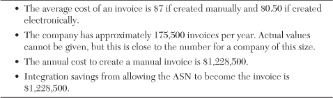
Table 4-6. Comparison of Invoice Created Manually and One Created Automatically by ASN

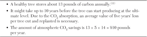
Table 4-7. Conversion of Number of Trees to Pounds of CO₂

Table 4-8. VMI Payback in Terms of Green Deployment

Table 4-9. Savings of Carrying Cost

Table 4-10. TMS and 3PL on CO₂: The Savings in Gasoline and CO₂ Emissions

Current progress from implementation of the TMS:

• Lean Savings

Inventory reduction is 5% × $206 million inventory = $10.3 million reduction.

Cost carrying reduction is $2.739 million.

Freed-up capital is 2% × $10.3 million inventory savings = $206,000.

Freight rate for consolidation savings is $4,527,270.

Freight rate savings from rate comparisons and rate shopping is $6,338,178.

Gasoline savings is 8% × 3.4 million gallons per year × $3.12 = $848,640.

New turns are $931 million / $196 million = 4.75 turns.

New inventory is at $196 million.

The Total Lean Savings is $14,659,088.

• Green Savings

Damaged inventory cost represents .75% of $10 million inventory = $75,000.

Obsolete inventory cost reduction is 9% of inventory reduction = $900,000.

Route optimization techniques save 3,019 tons of CO₂ from being released into the atmosphere.⁽¹³⁾

The TMS savings in dollars to the infrastructure per year is .09% × $20,000,000,000 × 38.5^{(4) (6)} = $6,930,000.

Green Savings is 19 trucks × 9,600 cars × 5 days × 51 weeks = 46,512,000 reduced cars on the road per year.⁽²⁾

The Total Green Savings is $7,905,000.

Total savings for the TMS program is $22,564,088.

Summary Savings

• The total cumulative Lean Savings from the VMI process to the TMS process is $78,156,488. This represents 8.39% of sales saved.

• The total cumulative Green Savings from the VMI process to the TMS process is $26,296,336. This represents 2.82% of sales saved.

• The total cumulative Lean and Green Savings from the VMI process to the TMS process is $104,452,824. This represents 11.22% of sales.

• For every dollar spent on Lean, $0.34 in Green is earned. So 34% of all Lean Savings goes into Green Savings at this point. This is significant.

The total savings for the entire program is $16,025,906, as itemized here:

• Lean Savings is $14,659,088.

• Green Savings is $1,366,818.

• There are 14 trees saved per year. Using the data given in Table 4-7, 14 trees equates to 910 pounds of CO₂ saved per year.

• There are 46,512,000 fewer cars on the road per year.

• Route optimization techniques save 3,019 tons of CO₂ from being released into the atmosphere.

• The TMS savings in dollars to the infrastructure per year is .09% × $20,000,000,000 × .25⁽⁴⁾ = $45,000,000.

The total TMS Savings Metrics in sales is $931 million, and in new inventory is $196 million. The new company turns are $931,000,000 / $196,000,000 = 4.75. The combined savings for the TMS Program is Lean Savings of $14,659,088 and Green Savings of $1,366,818.

The following is a summary of the Green Savings and corresponding references:

The Intergovernmental Panel on Climate Change (IPCC) guidelines for calculating emissions inventories require that an oxidation factor be applied to the carbon content to account for a small portion of the fuel that is not oxidized into CO₂. For all oil and oil products, the oxidation factor used is 0.99 (99% of the carbon in the fuel is eventually oxidized, while 1% remains unoxidized).⁽¹⁾

Finally, to calculate the CO₂ emissions from a gallon of fuel, the carbon emissions are multiplied by the ratio of the molecular weight of CO₂ (m.w. 44) to the molecular weight of carbon (m.w.12): 44 / 12.⁽¹⁾

CO₂ emissions from a gallon of gasoline are 2,421 grams × 0.99 × (44 / 12) = 8,788 grams = 8.8 kg/gallon = 19.4 pounds/gallon.⁽¹⁾

CO₂ emissions from a gallon of diesel are 2,778 grams × 0.99 × (44 / 12) = 10,084 grams = 10.1 kg/gallon = 22.2 pounds/gallon.⁽¹⁾

Note: These calculations and the supporting data have associated variation and uncertainty. EPA may use other values in certain circumstances, and in some cases it may be appropriate to use a range of values.⁽¹⁾

⁽²⁾ http://ftp.dot.state.tx.us/pub/txdot-info/gbe/french_fry.pdf.

⁽³⁾ Source: Department of Transportation: http://www.eia.gov/emeu/rtecs/chapter3.html.

⁽⁴⁾ http://cboblog.cbo.gov/?p=97.

⁽⁵⁾ RITA, Table 1-32: U.S. Vehicle-Miles, http://www.bts.gov/publications/national_transportation_statistics/html/table_01_32.html.

⁽⁶⁾ http://www.fhwa.dot.gov/policy/hcas/final/five.htm.

⁽⁷⁾ Feb 1, 2002, http://www.eia.doe.gov/emeu/rtecs/chapter3.html.

⁽⁸⁾ http://www.project.org/info.php?recordID=443 or http://www.fhwa.dot.gov/policyinformation/travel/tvt/history.

⁽⁹⁾ U.S. Environmental Protection Agency, “Emission Facts: Greenhouse Gas Emissions from a Typical Passenger Vehicle,” http://www.epa.gov/oms/climate/420f05004.htm.

⁽¹⁰⁾ http://www.arboristsite.com/firewood-heating-wood-burning-equipment/86041.htm.

⁽¹¹⁾ http://apps.sd.gov/news/showDoc.aspx?i=4092.

⁽¹²⁾ “Carbon Content in Motor Vehicle Fuels” and “Calculating CO₂ Emissions,” http://www.epa.gov/oms/climate/420f05001.htm.

⁽¹³⁾ http://ops.fhwa.dot.gov/freight/freight_analysis/econ_methods/lcdp_rep/index.htm, http://www.epa.gov/oms/climate/420f05001.htm.