
19. Forecasting Methodology and Gamma Smoothing: A Solution to Better Accuracy to Maintain Lean and Green
Introduction of Gamma Smoothing
Gamma smoothing is the culmination of a detailed examination of past forecast programs and their failures. The primary focus of this concept is a holistic integration of the needs of fortune 500 companies worldwide. It has been in practice for 20 years and continues to prove its superiority with increased service levels, turns, and low inventory.
Description of the Theory and the Formulas
Gamma smoothing always includes an underlining trend indicator (TI) to minimize the chance of out-of-stocks. The TI is a parameter that tells the system to add more trend component to the forecast. This becomes an automatic trend-detection system. It is not a filter that has to wait for two or three periods to trip the system as some forecast systems require.
Gamma smoothing also avoids the stair-step process of evaluating the tracking signal (TS). The process is constantly evaluating the change in demand and is more responsive to the variation in demand when calculating safety stock. With gamma smoothing, the safety stock is calculated with the variability of the demand pattern in mind.
Start by calculating the Dispersion Measure of the demand pattern:
• At-1 is the actual demand for the last period.
• Ft-1 is the forecast for the last period’s demand.
• γ Gamma = the smoothing constant for gamma smoothing = .10.
• δ Delta = the smoothing constant used for trend smoothing = .20.
• P or percent changed = Dn / D(n-1), which is the most recent demand divided by the last period demand.
• Pt is the initial smoothed value of P to be used in TICUM mentioned in the following text.
• TI = a running average of the trend component of demand pattern for the years.
• TIcum = the cumulative trend over the time series.
• (DM) Dispersion Measure is defined as follows:
• DM t-1 = (At-1 / Ft-1 − 1) when At-1 / Ft-1 > 1.00. This formula is used when the actual demand is greater than the forecast.
• DM t-1 = (1 − At-1 / Ft-1) when At-1 / Ft-1 < 1.00. This formula is used when the actual demand is less than the forecast when measuring the magnitude of the actual demand as less than the forecast.
• Ft is the forecast for the Horizontal Gamma Soothing Model and it is calculated as follows:
If At-1 / Ft-1 < 1 then:
• DM t-1 = (1 − At-1 / Ft-1)
• Ft = (1 − DM t-1 * γ) * Ft-1
If At-1 / Ft-1 > 1 then:
• DM t-1 = (At-1 / Ft-1 − 1)
• Ft = (DM t-1 * γ + 1) * Ft-1
• The mathematics behind the trend pattern follows by using the trend indicator:
• P or percent changed = Dn / D(n-1), which is the most recent demand divided by the last period demand.
If P < .80 it is set to P = .80. This is a default value to limit the variation or noise in the system for the lower bounds.
If P > 1.2 then it is set to P = 1.2. This is a default value to limit the variation or noise in the system for the upper bounds.
For values ≥ .80 and ≤ 1.2 use the P = Dn / D(n-1) value. This variation is within the tolerance of the system. Do not filter any of the forecasts P or Percent changed values.
• Pt = the Percent changed, which is the initial smoothed value for P. The smoothing constant for P is called Delta δ. Here use the value of Delta δ = .20.
If P < 1 use Pt = (1 − P) * δ.
If P ≥ 1 use Pt = (P − 1) * δ.
• If the P value of the demand is Dn / D(n-1) = 1.10 this means a 10% increase from this period compared to the last.
• After the smoothed value, increase the cumulative trend by 2%. Pt = (1.1 − 1) * .2 = .02. This value is used as a multiplier of TIcum, which in this case would be TIcum * (1.02).
• For example:
• TI = trend indicator is the cumulative trend of P where P = Dt / Dt-1. This is the cumulative smoothed value of TIcum for the time series. The TIcum is smoothed and updated throughout the year.
• TIcum is calculated in two different ways:
If P < 1 then TIcum+1 = (1 − Pt) * TIcum.
If P > 1 then TIcum+1 = (1 + Pt) * TIcum.
If P = 1 TIcum is not changed.
• Assume that the TIcum value at this time is 1.04.
• Given the Pt = .02.
• Now calculate the new value for TIcum+1, which is (1 + Pt) * TIcum = 1.02 * 1.04 = 1.06.
• The TIcum is a multiplicative sum of the average trend in the time series throughout the series.
• The Forecast Gamma (FG) will now have a trend component for the time series, which is represented as Fn+1 = Fn * TIcum+1. This stands for the forecast without safety stock.
• The forecast with safety stock and trend is equal to FSN+1 = FN+1 * TIcum+1 + k * MAD * β, where beta β is the coefficient determined by the Volatility Index (VI). The VI is based on the relative variation in the forecast values over time. If the system has decreased volatility, use a lower value of beta β. This FSN+1 is called OQ G because the focus is to compute safety stock and eventually a forecast using gamma smoothing.
• Including lead time in the preceding equation to calculate the OQ order quantity changes the formula to OQ G = FN+1 * (LT + RT) * TIcum + k * MAD * (LT + RT) .7 * β.
A Comparison Using Gamma Smoothing and Exponentials Smoothing
Figure 19-1 shows the forecasts for exponential smoothing as FE and gamma smoothing as FG. FE and FG are the initial forecast without safety stock. The graph also shows the order quantity using exponential (OQ E) and gamma smoothing (OQ G), which includes the safety stock calculation. As a matter of convention, reference to an order quantity always includes the safety stock calculation in the forecast.
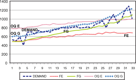
Figure 19-1. The comparison of exponential smoothing versus gamma smoothing without the TI
The data in Tables 19-1 has a slight trend that is not enough to trip the TS. But the TI picks it up in gamma smoothing. Figure 19-1 shows both the gamma smoothing and the exponential smoothing with and without the safety stock portion. Table 19-2 is without the use of the TI and it compares this to the Exponential Smoothing Model. The gamma smoothing can accelerate the findings of small trends that can go undetected in some systems. The results were simulated in an Excel spreadsheet and over time indicated the average turns and service levels.
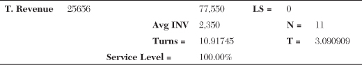
Table 19-1. The Exponential Smoothing Metrics for Figure 19-1
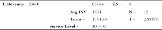
Table 19-2. The Gamma Smoothing Metrics Without TI and Beta at .50
Note that the differences in turns have accelerated between the exponential smoothing and gamma smoothing, from turns of 10.9 to 13.01. With the additional protection of the TI, the risk of out-of-stocks is reduced, making the forecast more accurate. This can be concluded by the lower MAD in the series as it was simulated over the past year. Reinitialization is necessary whenever a change is made to the forecast model to determine whether it is a better model. Because the MAD is lower, it’s necessary to simulate the new value for beta. In this model, a lower value for beta is used because the forecast is improved by the addition of the TI also shown graphically in Figure 19-2. The inclusion of the TI causes less variance in the forecast, which results in a lower MAD. The gamma smoothing metrics with TI uses a beta of .38 instead of the .50 used without the TI, as shown in Table 19-3.
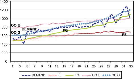
Figure 19-2. The gamma smoothing metrics with the use of the TI

Table 19-3. The Gamma Smoothing Metrics with TI and Beta at .38
Note that the gamma smoothing with the TI seems to get its turns from having a lower inventory in the beginning of the graph. As the trend begins to pick up, the OQ G picks up more sharply as compared to the previous graph without the trend indicator. To summarize, turns have improved from 13.01 to a value of 14.92 using the TI value. Note that the Order Quantity levels are higher at the end. This is because of the inclusion of the trend.
An Applied Example of the Gamma Smoothing Calculations over Time
If the demand in November was 500 and the forecast for November was 400 for an item carried by XYZ Retailer, then the actual demand in December was 600. What is the forecast for January when calculating in November? After December’s forecast is calculated, January’s can be done.
• At-1 for November = 500.
• At for December = 600.
• Ft-1 = 400.
• Gamma γ = .10. This is the gamma smoothing constant similar to α in exponential smoothing. In gamma smoothing, the γ is the smoothed average for the ratios of increase or decrease in the system between the actual demand and its forecast. In exponential smoothing, the α represents the smoothed average of the difference between the latest demand and the forecast for that period.
• Delta δ = .20 is used to smooth the trend component for TI.
• Calculate the forecast for December = Ft:
• Now At-1 / Ft-1 > 1 so
• DM t-1 = (At-1 / Ft-1 − 1) = (500 / 400 − 1) = 1.25 − 1.00 = .25
• The forecast for December is Ft = (DM t-1 * γ + 1) * Ft-1 = (.25 *.10 + 1) * 400 = (1.05) * 400 = 410.
• Calculate the forecast for January = Ft+1:
• Now At-1 / Ft-1 > 1 so
• DM t = (At / Ft − 1) = (600 / 410 − 1) = 1.46 − 1.00 − .46
• The forecast for January is Ft+1 = (DM t * γ + 1) * Ft = (.46 * .10 + 1) * 410 = (1.046) * 410 = 429.
• Introduce the TI for any possibility for trend to use as the TIcum for January.
• Assume that the TIcum = 1.06 for November.
• December demand = 600 and November demand = 500.
• P = Dt / Dt-1 = 600 / 500 = 1.2
• If P < 1 then
• Pt = (1 − P) * δ
• TIcum+1 = (1 - Pt) * TIcum
• If P > 1 then
• Pt = (P − 1) * δ = (1.2 − 1) * .2 = .04
• TIcum+1 = (1 + Pt) * TIcum
• TIcum+1 = (1 + Pt) * TIcum = (1 + .04) * 1.06 = 1.10
• The forecast for January is Fn+1 * TIcum+1 = 429 * 1.10 = 471.5.
The Trend Section of Gamma Smoothing Using TI
Gamma smoothing automates the trend model rather than forcing the user to wait for reinitialization notification. Gamma smoothing highlights the change in forecast models and reacts to it before a problem exists. This is especially true when using the trend indicator. If the actual demand gets larger or smaller than expected through time, the TI calculates the trend forecast system.
The system also measures various amounts of volatility in the demand pattern. This measurement is calibrated by the Volatility Index (VI), which equals MAD / AVG. The VI measures the volatility of the demand; the larger the value, the more volatility exists in the demand pattern. As the VI increases, so does the need to add extra safety stock.
VI will be valued at .069 and the gamma versus exponential smoothing results are graphed in Figure 19-3 to demonstrate this comparison.
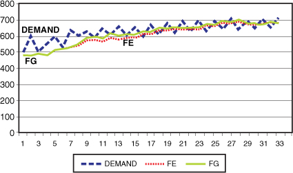
Figure 19-3. Graph using a VI = .069 and showing the gamma versus exponential smoothing
The value FE is the forecast value for exponential smoothing without safety stock. The value of FG is the forecast value for gamma smoothing without safety stock. Note that gamma smoothing corrects faster to the change in demand from demand periods 7 to 25. At the finish, both systems end up at approximately the same point. Both systems ride on the bottom edge of the demand pattern. This is the reason for safety stocks. The concept of ABCDE analysis discussed earlier can also be applied to improve the weighting values for safety stocks. The concept and calculation of safety stock will be covered in the dispersion section. The comparison begins with a very low-volatility demand pattern measured by the VI which equals .06845, as shown in Figure 19-4. As the chapter proceeds, the effects of safety stocks are measured with the different VIs compared in the next scenario of comparisons. The VI of .069 is very low, which indicates that the MAD does not deviate from the overall average very much.
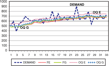
Figure 19-4. The graph of VI = 0.06845
Dispersion Measurement
This section discusses the concept of telling the computer what safety stock level is needed for the appropriate service level. Figure 19-4 shows a VI of 0.06845, which is a very low value indicating that the MAD variation compared to the average is 6.85% of the mean demand for the year. If confidence bands surrounded the mean, there would be a plus or minus 6.85% deviation around the mean. This is small so it’s considered a very stable demand that needs very little safety stock.
Add safety stock only selectively when it’s called for. Fast-moving items need only a small amount of safety stock because their pattern is so regular and this results in a low VI value. In most classic cases, more safety stock is added to the fast-moving items. This is not always necessary. It all depends on the volatility of the demand pattern. When demand is predictable, it makes sense to lower the safety stock level.
Figure 19-4 shows a demand pattern that moves from low to high. It also has a low VI which indicates that if the demand drops it will pick up in the near future. A low VI, in other words, says that the demand is predictable. This is called the wave pattern. When this pattern exists, the stock must be at a level that is a little higher than the wave patterns in the demand column. In this case, multiply the safety stock by the beta coefficient β. This is what makes gamma smoothing unique. There is a different beta coefficient for each VI. In this case, the VI is 0.06845. The beta used is .50. Beta is multiplied by the MAD to yield a reduced MAD. The new MAD = MAD * β, which = MAD * .5.
The next coefficient used is the k factor. This is used because of the importance of the item to overall service level, item demand, or profit margin. This was determined in the ABCDE hierarchy of inventory. The k values are in Chapter 21, “The New Sustainable EOQ Formula,” in Table 21-1, which gives the relationship of k to the Z transform. It’s necessary to balance the risk of the item with its priority or importance. The concept for determining safety stock is a two-step approach:
• Multiply MAD by β to get the correct risk factor for the demand pattern.
• Multiply MAD by k to get the correct service level for the ABCDE classification. How important is the item if sales are lost? What is its priority? This step converts the MAD into safety stock.
The safety stock is now prioritized by risk and priority.
For example, the calculation for safety stock is SS = k * MAD * β.
The demand pattern in Figure 19-5 follows a fairly predictable wave pattern. A larger value of VI is used for this example to illustrate the differences between the two systems. Exponential smoothing usually follows at the top of the wave pattern. It is marked as OQ E. The OQ G usually rides in the middle of the demand pattern. This is because it looks at the Volatility Index to check for a predictable wave pattern. It keeps the order quantity at midwave level, where half the demand will fall above and half will fall below. This assumes a stable wave pattern as measured by the VI indicator. If the demand drops, there is a reasonable probability it will increase in the next period or two. The converse is also accepted. If the demand increases, there is a reasonable probability that it will decrease in the next period or two.
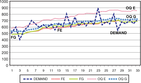
Figure 19-5. The graph of larger than VI = 0.06845
The β beta values are calculated from the VI as presented in the following bullet points. The list is only an example and each system requires its own analysis. To calculate, simulate the demand pattern history and use the beta values for a specific company. Those values may be different than the ones listed here:
• VI ≤ .10 yields β of .5 to .70 depending in the spikes in the demand. This means that the variation is less than 10% of the mean value for the time period.
• VI > .10 and ≤ .20 yields β of .50 to .80 depending in the spikes in the demand. This means that the variation is greater than 10% but less than or equal to 20% of the mean value for the time period.
• VI > .20 and ≤ .30 yields β of .50 to .80 depending in the spikes in the demand. This means that the variation is greater than 20% but less than or equal to 30% of the mean value for the time period.
• VI > .30 and ≤ .40 yields β of .50 to .80 depending in the spikes in the demand. This means that the variation is greater than 30% but less than or equal to 40% of the mean value for the time period.
• VI > .40 and ≤ .50 yields β of .50 to .80 depending in the spikes in the demand. This means that the variation is greater than 40% but less than or equal to 50% of the mean value for the time period.
• VI > .50 and ≤ 1.0 yields β of .50 to 1.0 depending in the spikes in the demand. This means that the variation is greater than 50% but less than or equal to 100% of the mean value for the time period.
• VI > 1.0 and ≤ 1.1 yields a β of .50 to 1.0 depending in the spikes in the demand. This means that the variation is greater than 100% but less than or equal to 110% of the mean value for the time period.
• VI > 1.1 indicates a need to check the TI, the TS tracking signal, the DF demand filter, and the OI for the outliner index. All of these are covered in the “Error Measurement” section later in this chapter. This means that the variation is greater than 110% of the mean value for the time period. This definitely needs more safety stock in the system to minimize the out-of-stock conditions.
Observing the Effects of Increasing the Volatility Index
This section graphs the various combinations of the Variability Index (VI). The section starts with VI ≤ .10 yields β of .50. This represents a point that is slightly above the average of the peaks and troughs of the demand pattern. The original VI from Figure 19-5 is 0.06845. Figure 19-6 shows an instance of VI = .0819, which is getting closer to .10, the first break point.
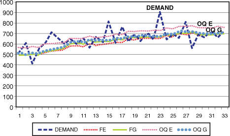
Figure 19-6. The graph of VI = .0819
The following list explains the values used in the forecast:
• Demand = the usage per the period.
• FE = the exponential smoothed forecast without safety stock.
• FG = the gamma smoothed forecast without safety stock.
• OQ E = the order quantity using exponential smoothing and including safety stocks.
• OQ G = the order quantity using gamma smoothing and including safety stocks.
Note that the OQ G is in the middle of the wave pattern and it is fairly consistent.
Figure 19-7 represents a VI of .10, and safety stock needs to be added because the volatility has increased from the VI of .0819. Note that as the VI indicator increases, the OQ E gap widens from the OQ G.
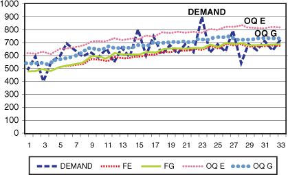
Figure 19-7. The graph of VI = .10
Notice as the VI increases to VI = .15 (Figure 19-8), the amplitude of the waves gets larger. Gamma smoothing is still at midlevel. The OQ G is still in the midrange of the demand patterns because the waves are still fairly predictable.
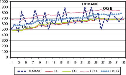
Figure 19-8. The graph of VI = .15
Amplitude increases as VI increases. A good service level exists because there are no real outliners and the waves are still predictable. This results in the OQ G being positioned in the middle of the demand patterns even with the large spikes in periods 10, 12, and 16 (Figure 19-9).
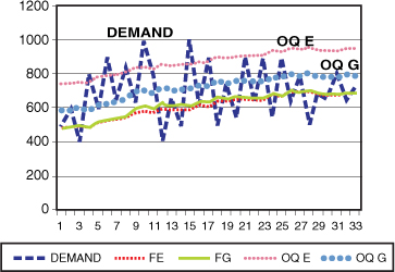
Figure 19-9. The graph of VI = .20
The next period requires additional safety stock analysis. Spikes should be analyzed to see whether they are occurring in a seasonal fashion. Are there any extraneous explanations to this sudden increase or decrease? Have inventory prices dropped or are there any promotions during this time? This is where inventory progress is made as long as there is no service-level sacrifice.
Inventory Control Metrics for Various VI Patterns
This section of the chapter compares the actual metrics in the various combinations of VI including the turns, number of times ordered, and service levels between the exponential smoothing systems and gamma smoothing systems using the various VI combinations. The section compares the Exponential Smoothing and Gamma Smoothing Models with the following combinations of VI at 0815, .20, .50, and finally at VI equal to 1.0. This section shows, in numerical terms, what happens to both systems as volatility goes up.
1. The following list compares the turns and service level for exponential smoothing and gamma smoothing.
2. Definitions:
• Demand = monthly demand.
• OQ E = order quantity for exponential smoothing, which is a one-period forecast.
• OQ = the OQ E multiplied by 4. As a standard, the company wants four periods of stock to be carried to cover lead time or any unexpected changes in demand. This is a normal procedure for most firms. The number of periods held in stock may change from one company to the next.
• OH = on hand.
• PO = purchase order created.
• Lost Sales = lost sales this period.
• n = 1 for any purchase orders created. This value is used in tracking the number of orders placed in the year.
• N = number of orders placed in the year.
• T = time between the orders.
Inventory at VI = .08187 with Exponential Smoothing and Gamma Smoothing
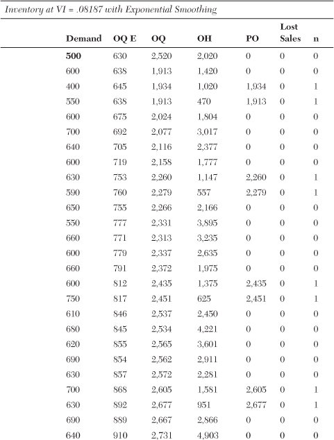
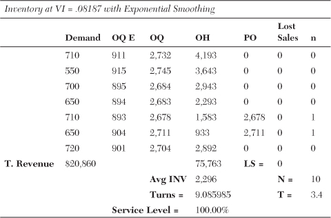
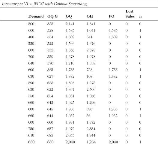
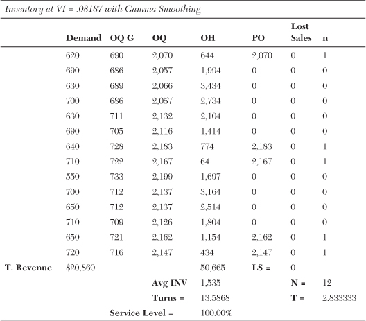
When comparing the two methods of forecasting, note that neither system experienced out-of-stocks or lost sales.
The Exponential Smoothing Model has the following benchmarks:
• Turns = 9.085.
• Lost Sales = 0.
• N = number of orders placed = 10.
• T = interval between orders = 3.4.
The Gamma Smoothing Model has the following benchmarks:
• Turns = 13.587.
• Lost Sales = 0.
• N = number of orders placed = 12.
• T = interval between orders = 2.8.
The difference becomes apparent. Gamma smoothing will increase the turns by 50%, from turns of 9.085 to turns of 13.587. There is also no sacrifice in lost sales. The number of orders placed throughout the year with gamma smoothing will also increase by 20%, from 10 to 12. This is because less stock is carried. If transportation is an issue, it will need to be addressed with higher stock levels.
Inventory at VI = .20 with Exponential Smoothing and Gamma Smoothing
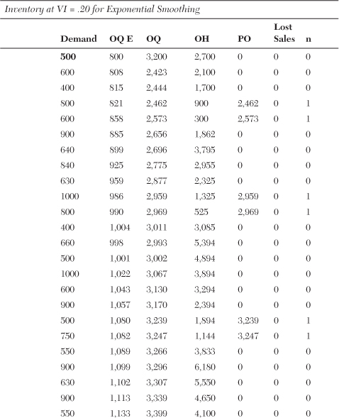
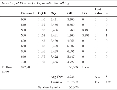
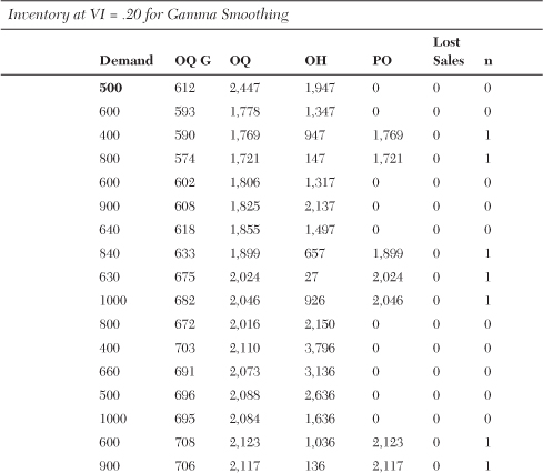
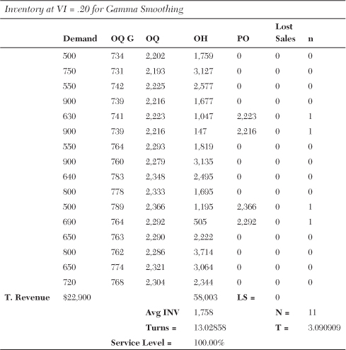
When the two methods of forecasting are compared, the difference is clear. Neither system experienced out-of-stocks, notated as LS for lost sales. The exponential smoothing has the following benchmarks:
• Turns = 7.
• Lost Sales = 0.
• N = number of orders placed = 8.
• T = interval between orders = 4.25.
The gamma smoothing has the following benchmarks:
• Turns = 13.03.
• Lost Sales = 0.
• N = number of orders placed = 11.
• T = interval between orders = 3.09.
Gamma smoothing will increase the turns by 84.1%, from turns of 7.075 to turns of 13.028. There is also no sacrifice in lost sales. The number of orders placed throughout the year will also increase by 38%, from 8 to 11.
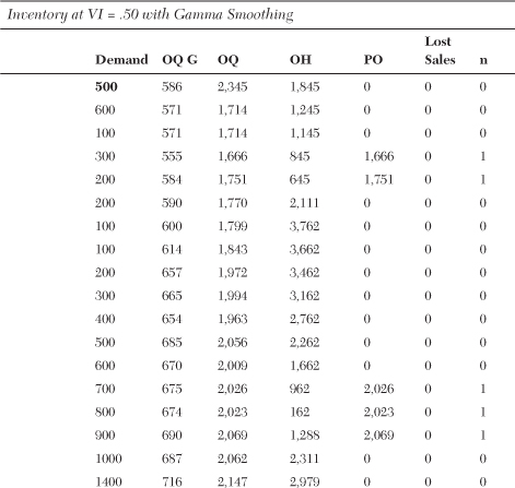
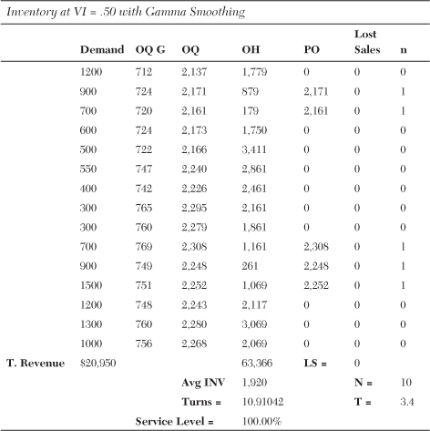
Inventory at VI = .50 with Exponential Smoothing and Gamma Smoothing
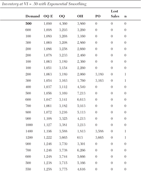
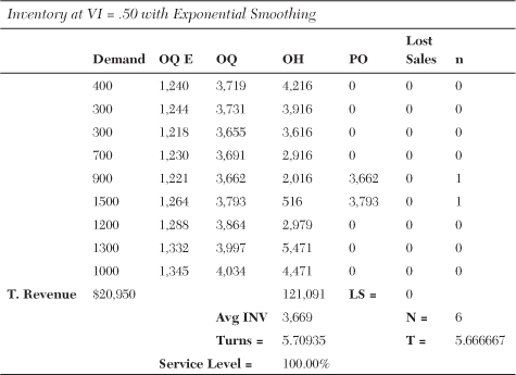
When comparing the two methods of forecasting, notice that neither system experienced out-of-stocks. The exponential smoothing mode has the following benchmarks:
• Turns = 5.71.
• Lost Sales = 0.
• N = number of orders placed = 6.
• T = interval between orders = 5.66.
The gamma smoothing has the following benchmarks:
• Turns = 10.91.
• Lost Sales = 0.
• Service Level = 100%
• N = number of orders placed = 10.
• T = interval between orders = 3.4.
Gamma smoothing increases the turns by 53%, from turns of 5.71 to turns of 10.91. There is also no sacrifice in lost sales. Exponential smoothing and gamma smoothing had a 100% service level. The number of orders placed throughout the year will also increase by 66.67%, from 6 to 10.
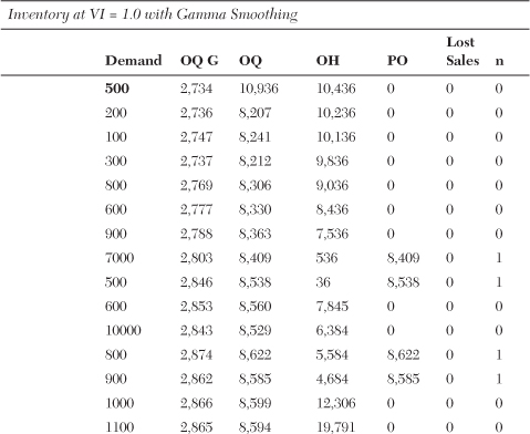
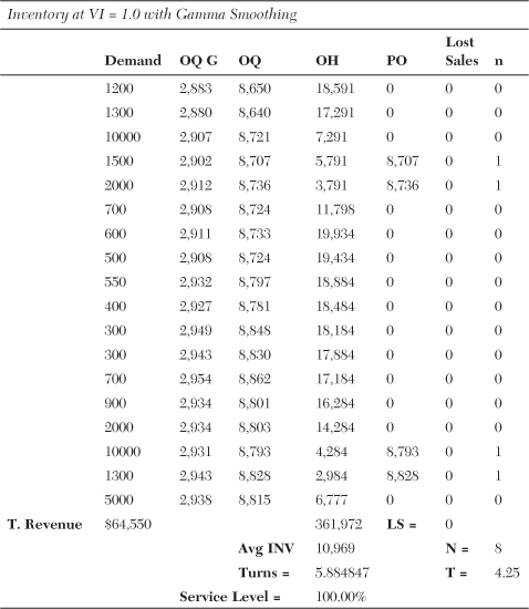
Inventory at VI = 1.0 with Exponential Smoothing and Gamma Smoothing
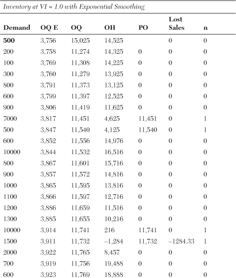
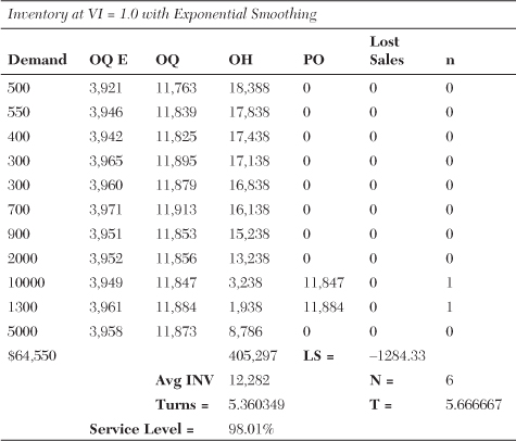
When comparing the two methods of forecasting, notice that neither system experienced out-of-stocks. The exponential smoothing mode has the following benchmarks:
• Turns = 5.36.
• Lost Sales = $1,284.
• Service Level = 98.1%.
• N = number of orders placed = 6.
• T = interval between orders = 5.66.
The gamma smoothing has the following benchmarks:
• Turns = 5.89.
• Lost Sales = 0.
• Service Level = 100%.
• N = number of orders placed = 8.
• T = interval between orders = 4.25.
Gamma smoothing will increase the turns by 10%, from turns of 5.36 to turns of 5.89. In the Exponential Smoothing Model, there are lost sales of 1.99%. The dollar amount of lost sales is $1,284. The service level is still high in the Exponential Smoothing Model at 98.01%. There is no sacrifice in lost sales for the Gamma Smoothing Model. The service level for gamma smoothing is 100%. The number of orders placed throughout the year will also increase by 33%, from 6 to 8, with gamma smoothing.
Turns began to fall at each level of VI for the Exponential Smoothing Model. At VI = .5 and VI = 1.0 the turns seemed to plateau on the low side at five plus turns. The Gamma Smoothing Model also decreased in turns as the VI increased but not as fast as the Exponential Smoothing Model. The Gamma Smoothing Model received its worst turns when VI = 1.0. The Gamma and Exponential Smoothing Models were close in turns at VI = 1. Normally, as the Volatility Index increases, the spread between the turns of exponential smoothing versus gamma smoothing increases in favor of gamma smoothing. In the last case where VI = 1.0, the spread between exponential smoothing and gamma smoothing was close due to the spikes in demand. This is registered by the outliner index (OI).
In this case the OI registered at 4. The OI monitors the number of outliners in the forecast. An outliner indicates that the demand is beyond the forecast’s capability to measure. Because the outliner cannot be measured, it represents an unpredictable spike or decrease in demand that cannot be forecasted in the model. To make things worse, the 4 out of 32 demand buckets indicates an incapability to measure demand on 12.5% of the demand series. Each increment of the OI will add significantly to the extra safety stock carried by the gamma smoothing. In this case, it’s necessary to carry extra safety stock because there are four instances in which the demand can’t be forecasted. This also explains the decrease in turns.
VI = 1.0
• The OI outliner index = 4 in the system. This means that there are four large spikes in demand. Figure 19-10 illustrates the four OI outliners on the demand line.
• FE = forecast using exponential smoothing without safety stocks.
• FG = forecast using gamma smoothing without safety stocks.
• OQ E = the order quantity for exponential smoothing, forecast plus safety stock.
• OQ G = the order quantity for gamma smoothing forecast plus safety stock.
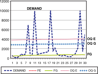
Figure 19-10. The graph showing the four outliners
Seasonal Exponential Smoothing and Seasonal Gamma Smoothing
The seasonal model uses base indexes for the monthly usage. It averages out the last three years’ monthly usages to create 12 monthly averages. Then divide each monthly average by the three year overage average to create 12 monthly base indexes. The reason for using the last three years’ usage is that it averages out late or early seasonal patterns.
How is forecasting using exponential smoothing and using the Ft value done? Ft stands for the current forecast for the current month. Ft+1 stands for the next month’s forecast. Table 19-4 is used for creating the appropriate forecast and base index values for the forecast.
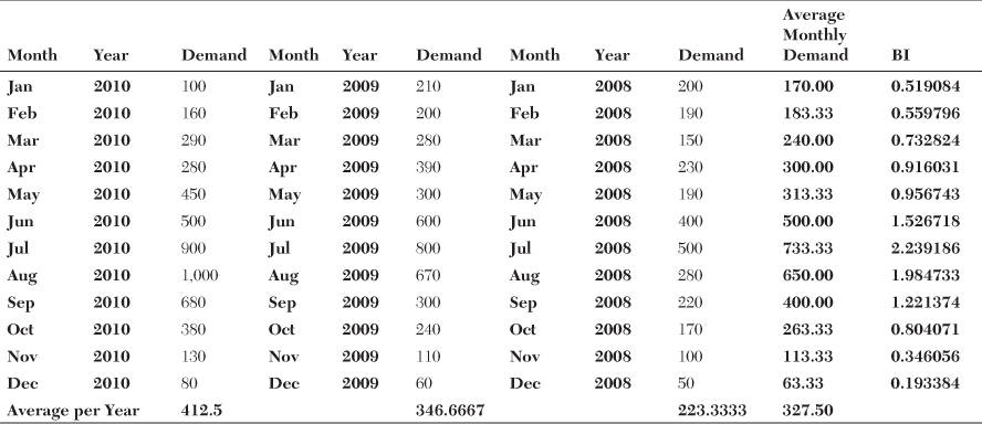
Table 19-4. Calculation of Initial Base Indexes (BI)
Table 19-4 shows the usages for three years and will be used in the calculations.
The average demand for all three years is equal to 327.50. Looking at the example of December 2010, the FDt for December is the overall average of 327.50, and the base index for December is equal to .1933. Both gamma smoothing and exponential smoothing use the concept of deseasonalized averages, termed FD to create the forecast.
All values calculating the demand for January, February, and March of 2011 will be smoothed in the future. Table 19-4 shows how to create the process. In forecasting terminology this is called initialization. Initialization is the creation of all the default values necessary to begin the forecasting and the eventual smoothing of all the values for future forecasts.
In this example are the forecasts for January, February, and March starting in December for exponential smoothing.
• FDDec stands for the new average for December and the average again is 327.50.
• FDJan stands for the new average for January after the month is complete.
• The alpha used in the smoothing of base index values and deseasonalized demand is .20.
• After January is completed, calculate the new deseasonalized demand for January = FDJan.
• ADec = the actual demand for December.
• FSJan = the seasonal forecast for January, which is FST+1 = FDT * BIT-11. Note that the BIT-11 says to use the base index 11 months back from December, which would be January 2010. The BI is .15908. So the new forecast for January 2011 or FSJan = FDDec * BIJan 2010 = 327.50 * .15908 = 170.
• FSJAN stands for January seasonalized forecast.
• After January’s demand is set at 130, the two contents of exponential smoothing can be considered.
• Next, smooth the forecast for changes in demand. Update the FD and BI constants:
• BIJan 2011 = AJan 2011 / FDDec 2010 = 130 / 327.50 = 0.397.
• Smoothed BIJan 2010 = 0.519084 + .20 * (0.397 − 0.519) = 0.495. This is the new smoothed base index for January 2011. This is the BI for the year when forecasting for January 2012.
• FDJan 2011 = (FDDec + .2 * (AJan 2010 / (BIJan 2010) − FDDec 2010) = 327.50 + .20 * (130 / 0.519084 − 327.50) = 351.588.
• After January is complete, it is time to calculate the forecast for February.
• The new forecast for February is FSFeb 2011 = BIFeb2010 * FDJan 2011 = 0.559796 * 351.588 = 196.818.
• FSFeb stands for February seasonalized forecast.
• Smooth the forecast for changes in demand. Update the FD and BI constants:
• BIFeb 2011 = AFeb 2011 / FDJan 2011 = 200 / 351.588 = 0.569.
• Smoothed BIFeb 2011 = 0.560 + .20 * (0.569 − 0.560) = 0.5616368. This is the new BI for February 2011. This is the BI used next year when forecasting for February 2012.
• FDFeb 2011 = (FDJan 2011 + .2 * (AFeb 2010 / (BIFeb 2010) − FDJan 2011) = (351.588 − .20 * (200 / 0.559796 − 351.588) = 352.725.
• After February’s demand is calculated, March’s forecast can be determined.
• The new forecast for March is FSMar 2011 = BIMar 2010 * FDFeb 2011 = 0.732824 * 352.725 = 258.4853454.
• FSMar 2011 stands for March seasonalized forecast.
• Next, smooth the forecast for changes in demand. Update the FD and BI constants:
• BIMar 2011 = AMar 2011 / FDFeb 2011 = 380 / 352.725 = 1.077.
• Smoothed BIMar 2011 = 0.733 + .20 * (1.077 − 0.733) = 0.801. This is the BI used next year when forecasting for March 2012.
• FDMar 2011 = (FDFeb 2011 + .2 * (AMar 2010 / (BIMar 2010) − FDFeb 2011) = (352.725 − .20 * (380 / 0.732824 − (352.725) = 385.888.
Another calculation that can be utilized is the demand for the next three months, January through March. If starting in December, the equation is FS(J to M) = FDDec * (BIt-11 + BIt-10 + BIt-9). This calculates the seasonalized demand for January through March.
Figures 19-11 and 19-12 show the difference between exponential smoothing and gamma smoothing. In gamma smoothing, the calculated BI for the month required taking the actual demand for the month and dividing it by the 12-month average demand. This is performed each month. The monthly average is the new FD. To calculate the new forecast for the next month, use the following formula:
This is done instead of smoothing the BI from period to period as was done previously. The big difference in the two algorithms is that the gamma smoothing system measures the Volatility Index and prorates the safety stock based on the degree of predictability in the demand patterns. Again, the formula for VI = MAD / (Average Demand). The Average Demand is for 12 months. The VI is 1.304 and this indicates a use of 40% of the safety stock values because the pattern is still predictable. As the VI gets larger, greater amounts of safety stock are necessary. For a good comparison, Figure 19-11 graphs the exponential smoothing seasonal forecast, and Figure 19-12 graphs the gamma smoothing seasonal forecast.
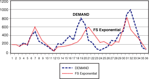
Figure 19-11. The exponential smoothing seasonal forecast
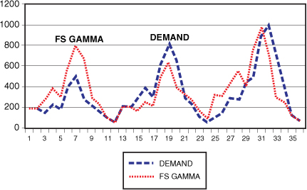
Figure 19-12. The gamma smoothing seasonal forecast
Figure 19-13 is a comparison of both exponential and gamma smoothing on the same graph versus demand. Note that in both models, the gamma smoothing does not lag as does the exponential smoothing. The Gamma Smoothing Model does initially include a lower amount of stock, which is based on the Volatility Index.
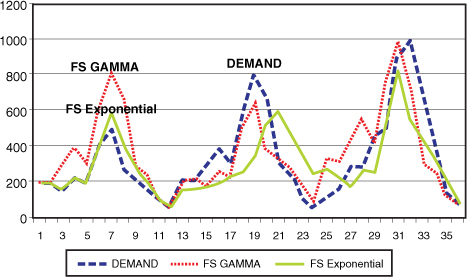
Figure 19-13. The graph compares exponential smoothing and gamma smoothing.
Graph of Exponential Smoothing Order Quantity
The order quantity is the forecast with safety stock added in for the Exponential Smoothing Model. The equation is OQS Exp = FS Exponential + k * MAD. The FS Exponential is the forecast seasonalized as described previously for the exponential model, where FSN+1 = FDN * BI(N − 11). The OQ Exponential = FSN+1 = FDN * BI(N-11) + k * MAD.
The formula for the forecast for gamma smoothing is FSN+1 = FDN * BI(N-12). The order quantity is the forecast with safety stock for the Exponential Smoothing Model. The OQ Gamma = FSN+1 = FDN * BI(N-12) + k * MAD * β, where beta β is the coefficient determined by the VI.
The Gamma Smoothing Model gives a closer fit to the demand pattern. This is because it measures the volatility of the demand pattern with the Volatility Index. This measures its predictability and reduces the need for unnecessary safety stock with the beta β coefficient.
Tables 19-5 and 19-6 show the effect on turns, number of times ordered, and inventory level using the two approaches. The order quantity (OQ) is the order quantity seasonalized and bought for three periods. This is a policy decision that can change from company to company. The three periods’ quantity is established to match the lead times and any large demand pattern.
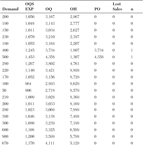
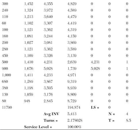
Table 19-5. Seasonal Exponential Smoothing
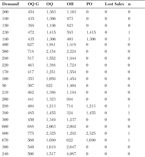
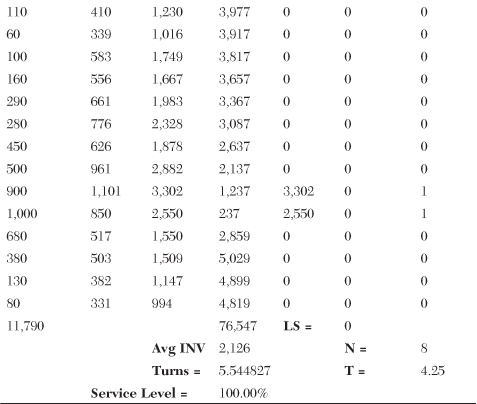
Table 19-6. Seasonal Gamma Smoothing
When comparing the two methods of forecasting, note that neither system experienced out-of-stocks, notated as LS for lost sales. The Exponential Smoothing Model has the following benchmarks:
• Turns = 2.18.
• Lost Sales = 0.
• Service Level = 100%.
• N = number of orders placed = 4.
• T = interval between orders = 8.5.
The gamma smoothing has the following benchmarks:
• Turns = 5.55.
• Lost Sales = 0.
• Service Level = 100%.
• N = number of orders placed = 8.
• T = interval between orders = 4.25.
Gamma smoothing increases the turns by 155%, from turns of 2.18 to turns of 5.55. There is no sacrifice in lost sales. The number of orders placed throughout the year increases by 100%, from four to eight.
Error Measurement
In this case, the VI is 0.06845. This results in beta β of .50. This figure is multiplied by the MAD to yield a reduced Mean Absolute Deviation. The new MAD = MAD * β, or MAD * .5. This measure is used with the k factor as well so that the user can selectively create the ABCDE hierarchy of inventory based on the importance of the item to overall sales. The theory requires a multiple-step approach:
• The Volatility Index measures the variation and degree of unpredictability:
• Multiply safety stock to get the correct risk profile for the demand pattern. This is determined by the VI and VI = MAD/AVG.
• VI is a measurement of instability in the demand pattern, and it dictates the need to add or subtract more safety stock from the system.
• Add safety stock only selectively when necessary. Many fast-moving items need only a small amount of safety stock because their pattern is so regular. In most classical cases, the experts say to add more safety stock to the fast-moving items. This is not necessarily true. It all depends on the volatility of the demand pattern.
• The VI indicates what beta β value to use to approximate the risk in volatility in the demand pattern.
• Priority is measured using the k factor:
• Next, multiply safety stock by k to get the correct service level for the ABCDE classification.
• The safety stock is now prioritized by risk and order of importance. When balancing both priorities, the new calculation for safety stock is SS = k * MAD * β.
• When including lead time (LT) and review time (RT) values of the Order Quantity, the formula becomes OQ = FS * (LT + RT) + k * MAD.7 * β.
• Taking the MAD components to the .7 power was determined to give the best multiplicative coefficient for the lead-time variability on MAD. To simulate this, multiply MAD for both the exponential smoothing and the gamma smoothing by a constant equal to .764.
• Outliner Indicator (OI):
• This system checks for outliners or spikes in the demand pattern that cannot be anticipated.
• OI = Dt / AVGt
• Dt = the current demand.
• AVGt = the average demand for the last month.
• If OI > 3 then this is an exception and the OI is set from 0 to 1.
• This system counts how many times in a rolling year there is an exception.
• It increases the safety stock level for the system as follows:
• Safety stock = k * MAD * (β + .1 * OI). This could change by system. If it changes, use a different coefficient other than the .1, for example .15 or .20 value.
• If the Volatility Index states a beta of .5 with three exceptions, or OI = 3 throughout the year, the new beta will be equal to .80, or .5 + .3.= .8
• Updated safety stock is k * MAD * .8 = k * MAD * .7.
• Tracking signal indicator (TS):
• The tracking signal traces the running sum of errors (RSE) in the system. Over a period of time as these errors accumulate, they will show either upward or downward bias in the forecast system.
• The formula for the tracking signal is ![]()
• Any value greater than a 3 is a concern.
• Downward or upward bias can be tracked using the demand filter.
• Demand Filter (DF):
• DF = cumulative forecast error divided by the MAD. The formula notation is ![]() .
.
• A value of DF > 6 will trip the Demand Filter device.
• This option checks how many MADs are over or under in the forecast.
• Any value above a 6 or below a –6 is a concern. The filters of plus or minus 6 are not cast in concrete. A 4 or 5 may also be used, depending on the importance of demand change.
• Error measurement is the process of closing the loop in the system. It will notify the user when one of the following conditions arises:
• Forecast is erroneous.
• There exists spurious demand.
• The demand pattern is changing.
• The beginning of a fad is present.
• Similar items are on promotion.
• A competitor advertised the items.