3. An Introduction to Classification

Overview

This chapter introduces you to classification. You will implement various techniques, such as k-nearest neighbors and SVMs. You will use the Euclidean and Manhattan distances to work with k-nearest neighbors. You will apply these concepts to solve intriguing problems such as predicting whether a credit card applicant has a risk of defaulting and determining whether an employee would stay with a company for more than two years. By the end of this chapter, you will be confident enough to work with any data using classification and come to a certain conclusion.

Introduction

In the previous chapter, you were introduced to regression models and learned how to fit a linear regression model with single or multiple variables, as well as with a higher-degree polynomial.

Unlike regression models, which focus on learning how to predict continuous numerical values (which can have an infinite number of values), classification, which will be introduced in this chapter, is all about splitting data into separate groups, also called classes.

For instance, a model can be trained to analyze emails and predict whether they are spam or not. In this case, the data is categorized into two possible groups (or classes). This type of classification is also called binary classification, which we will see a few examples of in this chapter. However, if there are more than two groups (or classes), you will be working on a multi-class classification (you will come across some examples of this in Chapter 4, An Introduction to Decision Trees).

But what is a real-world classification problem? Consider a model that tries to predict a given user's rating for a movie where this score can only take values: like, neutral, or dislike. This is a classification problem.

In this chapter, we will learn how to classify data using the k-nearest neighbors classifier and SVM algorithms. Just as we did for regression in the previous chapter, we will build a classifier based on cleaned and prepared training data and test the performance of our classifier using testing data.

We'll begin by looking at the fundamentals of classification.

The Fundamentals of Classification

As stated earlier, the goal of any classification problem is to separate the data into relevant groups accurately using a training set. There are a lot of applications of such projects in different industries, such as education, where a model can predict whether a student will pass or fail an exam, or healthcare, where a model can assess the level of severity of a given disease for each patient.

A classifier is a model that determines the label (output) or value (class) of any data point that it belongs to. For instance, suppose you have a set of observations that contains credit-worthy individuals, and another one that contains individuals that are risky in terms of their credit repayment tendencies.

Let's call the first group P and the second one Q. Here is an example of such data:

Figure 3.1: Sample dataset

With this data, you will train a classification model that will be able to correctly classify a new observation into one of these two groups (this is binary classification). The model can find patterns such as a person with a salary above $60,000 being less risky or that having a mortgage/income ratio above ratio 10 makes an individual more at risk of not repaying their debts. This will be a multi-class classification exercise.

Classification models can be grouped into different families of algorithms. The most famous ones are as follows:

• Distance-based, such as k-nearest neighbors
• Linear models, such as logistic regression or SVMs
• Tree-based, such as random forest

In this chapter, you will be introduced to two algorithms from the first two types of family: k-nearest neighbors (distance-based) and SVMs (linear models).

Note

We'll walk you through tree-based algorithms such as random forest in Chapter 4, An Introduction to Decision Trees.

But before diving into the models, we need to clean and prepare the dataset that we will be using in this chapter.

In the following section, we will work on a German credit approvals dataset and perform all the data preparation required for the modeling stage. Let's start by loading the data.

Exercise 3.01: Predicting Risk of Credit Card Default (Loading the Dataset)

In this exercise, we will be loading a dataset into a pandas DataFrame and exploring its contents. We will use the dataset of German credit approvals to determine whether an individual presents a risk of defaulting.

Note

The CSV version of this dataset can be found on our GitHub repository:

https://packt.live/3eriWTr.

The original dataset and information regarding the dataset can be found at https://archive.ics.uci.edu/ml/datasets/Statlog+%28German+Credit+Data%29.

The data files are located at https://archive.ics.uci.edu/ml/machine-learning-databases/statlog/german/.

Citation - Dua, D., & Graff, C.. (2017). UCI Machine Learning Repository.

1. Open a new Jupyter Notebook file.
2. Import the pandas package as pd:

   import pandas as pd

3. Create a new variable called file_url, which will contain the URL to the raw dataset file, as shown in the following code snippet:

   file_url = 'https://raw.githubusercontent.com/'

              'PacktWorkshops/'

              'The-Applied-Artificial-Intelligence-Workshop/'

              'master/Datasets/german_credit.csv'

4. Import the data using the pd.read_csv() method:

   df = pd.read_csv(file_url)

5. Use df.head() to print the first five rows of the DataFrame:

   df.head()

   The expected output is this:

   

   Figure 3.2: The first five rows of the dataset

   As you can see, the output in the preceding screenshot shows us the features of the dataset, which can be either numerical or categorical (text).

6. Now, use df.tail() to print the last five rows of the DataFrame:

   df.tail()

   The expected output is this:

   

   Figure 3.3: The last five rows of the dataset

   The last rows of the DataFrame are very similar to the first ones we saw earlier, so we can assume the structure is consistent across the rows.

7. Now, use df.dtypes to print the list of columns and their data types:

   df.dtypes

   The expected output is this:

   

Figure 3.4: The list of columns and their data types

Note

To access the source code for this specific section, please refer to https://packt.live/3hQXJEs.

You can also run this example online at https://packt.live/3fN0DrT. You must execute the entire Notebook in order to get the desired result.

From the preceding output, we can see that this DataFrame has some numerical features ( int64) but also text (object). We can also see that most of these features are either personal details for an individual, such as their age, or financial information such as credit history or credit amount.

By completing this exercise, we have successfully loaded the data into the DataFrame and had a first glimpse of the features and information it contains.

In the topics ahead, we will be looking at preprocessing this data.

Data Preprocessing

Before building a classifier, we need to format our data so that we can keep relevant data in the most suitable format for classification and remove all the data that we are not interested in.

The following points are the best ways to achieve this:

• Replacing or dropping values:

  For instance, if there are N/A (or NA) values in the dataset, we may be better off substituting these values with a numeric value we can handle. Recall from the previous chapter that NA stands for Not Available and that it represents a missing value. We may choose to ignore rows with NA values or replace them with an outlier value.

  Note

  An outlier value is a value such as -1,000,000 that clearly stands out from regular values in the dataset.

  The fillna() method of a DataFrame does this type of replacement. The replacement of NA values with an outlier looks as follows:

  df.fillna(-1000000, inplace=True)

  The fillna() method changes all NA values into numeric values.

  This numeric value should be far from any reasonable value in the DataFrame. Minus one million is recognized by the classifier as an exception, assuming that only positive values are there, as mentioned in the preceding note.

• Dropping rows or columns:

  The alternative to replacing missing values with extreme values is simply dropping these rows:

  df.dropna(0, inplace=True)

  The first argument (value 0) specifies that we drop rows, not columns. The second argument (inplace=True) specifies that we perform the drop operation without cloning the DataFrame, and will save the result in the same DataFrame. This DataFrame doesn't have any missing values, so the dropna() method didn't alter the DataFrame.

  Note

  Dropping the NA values is less desirable, as you often lose a reasonable chunk of your dataset.

  If there is a column we do not want to include in the classification, we are better off dropping it. Otherwise, the classifier may detect false patterns in places where there is absolutely no correlation.

  For instance, your phone number itself is very unlikely to correlate with your credit score. It is a 9 to 12-digit number that may very easily feed the classifier with a lot of noise. So, we can drop the telephone column, as shown in the following code snippet:

  df.drop(['telephone'], 1, inplace=True)

  The second argument (value 1) indicates that we are dropping columns, instead of rows. The first argument is an enumeration of the columns we would like to drop (here, this is ['telephone']). The inplace argument is used so that the call modifies the original DataFrame.

• Transforming data:

  Often, the data format we are working with is not always optimal for the classification process. We may want to transform our data into a different format for multiple reasons, such as to highlight aspects of the data we are interested in (for example, Minmax scaling or normalization), to drop aspects of the data we are not interested in (for example, binarization), label encoding to transform categorical variables into numerical ones, and so on.

  Minmax scaling scales each column in the data so that the lowest number in the column becomes 0, the highest number becomes 1, and all of the values in-between are proportionally scaled between 0 and 1.

  This type of operation can be performed by the MinMaxScaler method of the scikit-learn preprocessing utility, as shown in the following code snippet:

  from sklearn import preprocessing

  import numpy as np

  data = np.array([[19, 65],

                   [4, 52],

                   [2, 33]])

  preprocessing.MinMaxScaler(feature_range=(0,1)).fit_transform(data)

  The expected output is this:

  array([[1. , 1. ],

         [0.11764706, 0.59375 ],

         [0. , 0. ]])

  Binarization transforms data into ones and zeros based on a condition, as shown in the following code snippet:

  preprocessing.Binarizer(threshold=10).transform(data)

  The expected output is this:

  array([[1, 1],

         [0, 1],

         [0, 1]])

In the preceding example, we transformed the original data ([19, 65],[4, 52],[2, 33]) into a binary form based on the condition of whether each value is greater than 10 or not (as defined by the threshold=10 parameter). For instance, the first value, 19, is above 10, so it is replaced by 1 in the results.

Label encoding is important for preparing your features (inputs) for the modeling stage. While some of your features are string labels, scikit-learn algorithms expect this data to be transformed into numbers.

This is where the preprocessing library of scikit-learn comes into play.

Note

You might have noticed that in the credit scoring example, there were two data files. One contained labels in string form, while the other contained labels in integer form. We loaded the data with string labels so that you got some experience of how to preprocess data properly with the label encoder.

Label encoding is not rocket science. It creates a mapping between string labels and numeric values so that we can supply numbers to scikit-learn, as shown in the following example:

from sklearn import preprocessing

labels = ['Monday', 'Tuesday', 'Wednesday',

          'Thursday', 'Friday']

label_encoder = preprocessing.LabelEncoder()

label_encoder.fit(labels)

Let's enumerate the encoding:

[x for x in enumerate(label_encoder.classes_)]

The expected output is this:

[(0, 'Friday'),

 (1, 'Monday'),

 (2, 'Thursday'),

 (3, 'Tuesday'),

 (4, 'Wednesday')]

The preceding result shows us that scikit-learn has created a mapping for each day of the week to a respective number; for example, Friday will be 0 and Tuesday will be 3.

Note

By default, scikit-learn assigned the mapping number by sorting the original values alphabetically. This is why Friday is mapped to 0.

Now, we can use this mapping (also called an encoder) to transform data.

Let's try this out on two examples, Wednesday and Friday, using the transform() method:

label_encoder.transform(['Wednesday', 'Friday'])

The expected output is this:

array([4, 0], dtype=int64)

As expected, we got the results 4 and 0, which are the mapping values for Wednesday and Friday, respectively.

We can also use this encoder to perform the inverse transformation with the inverse_transform function. Let's try this with the values 0 and 4:

label_encoder.inverse_transform([0, 4])

The expected output is this:

array(['Friday', 'Wednesday'], dtype='<U9')

As expected, we got back the values Friday and Wednesday. Now, let's practice what we've learned here on the German dataset.

Exercise 3.02: Applying Label Encoding to Transform Categorical Variables into Numerical Variables

In this exercise, we will use one of the preprocessing techniques we just learned, label encoding, to transform all categorical variables into numerical ones. This step is necessary before training any machine learning model.

Note

We will be using the same dataset that we used in the previous exercise: the German credit approval dataset: https://packt.live/3eriWTr.

The following steps will help you complete this exercise:

1. Open a new Jupyter Notebook file.
2. Import the pandas package as pd:

   import pandas as pd

3. Create a new variable called file_url, which will contain the URL to the raw dataset:

   file_url = 'https://raw.githubusercontent.com/'

              'PacktWorkshops/'

              'The-Applied-Artificial-Intelligence-Workshop/'

              'master/Datasets/german_credit.csv'

4. Load the data using the pd.read_csv() method:

   df = pd.read_csv(file_url)

5. Import preprocessing from scikit-learn:

   from sklearn import preprocessing

6. Define a function called fit_encoder() that takes a DataFrame and a column name as parameters and will fit a label encoder on the values of the column. You will use .LabelEncoder() and .fit() from preprocessing and .unique() from pandas (this will extract all the possible values of a DataFrame column):

   def fit_encoder(dataframe, column):

       encoder = preprocessing.LabelEncoder()

       encoder.fit(dataframe[column].unique())

       return encoder

7. Define a function called encode() that takes a DataFrame, a column name, and a label encoder as parameters and will transform the values of the column using the label encoder. You will use the .transform() method to do this:

   def encode(dataframe, column, encoder):

       return encoder.transform(dataframe[column])

8. Create a new DataFrame called cat_df that contains only non-numeric columns and print its first five rows. You will use the .select_dtypes() method from pandas and specify exclude='number':

   cat_df = df.select_dtypes(exclude='number')

   cat_df.head()

   The expected output (not all columns are shown) is this:

   

   Figure 3.5: First five rows of the DataFrame containing only non-numeric columns

9. Create a list called cat_cols that contains the column name of cat_df and print its content. You will use .columns from pandas to do this:

   cat_cols = cat_df.columns

   cat_cols

   The expected output is this:

   Index(['account_check_status', 'credit_history', 'purpose',

          'savings', 'present_emp_since', 'other_debtors',

          'property', 'other_installment_plans', 'housing',

          'job', 'telephone', 'foreign_worker'], dtype='object')

10. Create a for loop that will iterate through each column from cat_cols, fit a label encoder using fit_encoder(), and transform the column with the encode() function:

    for col in cat_cols:

        label_encoder = fit_encoder(df, col)

        df[col] = encode(df, col, label_encoder)

11. Print the first five rows of df:

    df.head()

    The expected output is this:

    

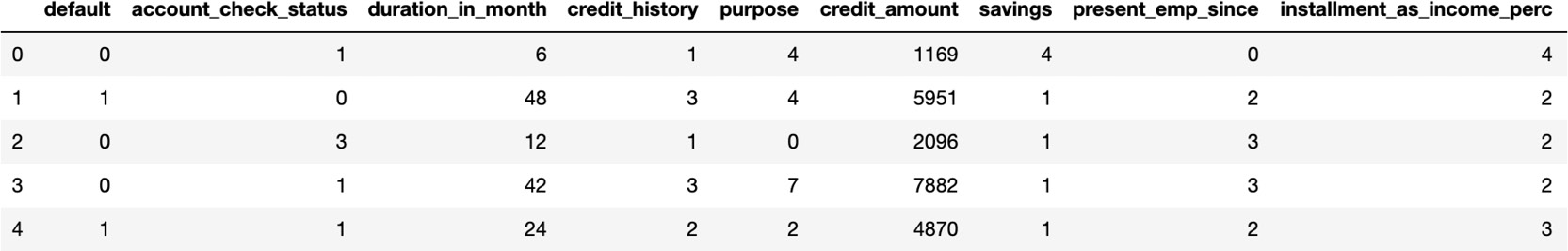
Figure 3.6: First five rows of the encoded DataFrame

Note

To access the source code for this specific section, please refer to https://packt.live/2Njh57h.

You can also run this example online at https://packt.live/2YZhtx5. You must execute the entire Notebook in order to get the desired result.

We have successfully encoded non-numeric columns. Now, our DataFrame contains only numeric values.

Identifying Features and Labels

Before training our model, we still have to perform two final steps. The first one is to separate our features from the label (also known as a response variable or dependent variable). The label column is the one we want our model to predict. For the German credit dataset, in our case, it will be the column called default, which tells us whether an individual will present a risk of defaulting or not.

The features are all the other columns present in the dataset. The model will use the information contained in those columns and find the relevant patterns in order to accurately predict the corresponding label.

The scikit-learn package requires the labels and features to be stored in two different variables. Luckily, the pandas package provides a method to extract a column from a DataFrame called .pop().

We will extract the default column and store it in a variable called label:

label = df.pop('default')

label

The expected output is this:

0 0

1 1

2 0

3 0

4 1

..

995 0

996 0

997 0

998 1

999 0

Name: default, Length: 1000, dtype: int64

Now, if we look at the content of df, we will see that the default column is not present anymore:

df.columns

The expected output is this:

Index(['account_check_status', 'duration_in_month',

       'credit_history', 'purpose', 'credit_amount',

       'savings', 'present_emp_since',

       'installment_as_income_perc', 'other_debtors',

       'present_res_since', 'property', 'age',

       'other_installment_plans', 'housing',

       'credits_this_bank', 'job', 'people_under_maintenance',

       'telephone', 'foreign_worker'],

      dtype='object')

Now that we have our features and labels ready, we need to split our dataset into training and testing sets.

Splitting Data into Training and Testing Using Scikit-Learn

The final step that's required before training a classifier is to split our data into training and testing sets. We already saw how to do this in Chapter 2, An Introduction to Regression:

from sklearn import model_selection

features_train, features_test,

label_train, label_test =

model_selection.train_test_split(df, label, test_size=0.1,

                                 random_state=8)

The train_test_split method shuffles and then splits our features and labels into a training dataset and a testing dataset.

We can specify the size of the testing dataset as a number between 0 and 1. A test_size of 0.1 means that 10% of the data will go into the testing dataset. You can also specify a random_state so that you get the exact same split if you run this code again.

We will use the training set to train our classifier and use the testing set to evaluate its predictive performance. By doing so, we can assess whether our model is overfitting and has learned patterns that are only relevant to the training set.

In the next section, we will introduce you to the famous k-nearest neighbors classifier.

The K-Nearest Neighbors Classifier

Now that we have our training and testing data, it is time to prepare our classifier to perform k-nearest neighbor classification. After being introduced to the k-nearest neighbor algorithm, we will use scikit-learn to perform classification.

Introducing the K-Nearest Neighbors Algorithm (KNN)

The goal of classification algorithms is to divide data so that we can determine which data points belong to which group.

Suppose that a set of classified points is given to us. Our task is to determine which class a new data point belongs to.

In order to train a k-nearest neighbor classifier (also referred to as KNN), we need to provide the corresponding class for each observation on the training set, that is, which group it belongs to. The goal of the algorithm is to find the relevant relationship or patterns between the features that will lead to this class. The k-nearest neighbors algorithm is based on a proximity measure that calculates the distance between data points.

The two most famous proximity (or distance) measures are the Euclidean and the Manhattan distance. We will go through more details in the next section.

For any new given point, KNN will find its k nearest neighbor, see which class is the most frequent between those k neighbors, and assign it to this new observation. But what is k, you may ask? Determining the value of k is totally arbitrary. You will have to set this value upfront. This is not a parameter that can be learned by the algorithm; it needs to be set by data scientists. This kind of parameter is called a hyperparameter. Theoretically, you can set the value of k to between 1 and positive infinity.

There are two main best practices to take into consideration:

• k should always be an odd number. The reason behind this is that we want to avoid a situation that ends in a tie. For instance, if you set k=4 and it so happens that two of the neighbors of a point are from class A and the other two are from class B, then KNN doesn't know which class to choose. To avoid this situation, it is better to choose k=3 or k=5.
• The greater k is, the more accurate KNN will be. For example, if we compare the cases between k=1 and k=15, the second one will give you more confidence that KNN will choose the right class as it will need to look at more neighbors before making a decision. On the other hand, with k=1, it only looks at the closest neighbor and assigns the same class to an observation. But how can we be sure it is not an outlier or a special case? Asking more neighbors will lower the risk of making the wrong decision. But there is a drawback to this: the higher k is, the longer it will take KNN to make a prediction. This is because it will have to perform more calculations to get the distance between all the neighbors of an observation. Due to this, you have to find the sweet spot that will give correct predictions without compromising too much on the time it takes to make a prediction.

Distance Metrics With K-Nearest Neighbors Classifier in Scikit-Learn

Many distance metrics could work with the k-nearest neighbors algorithm. We will present the two most frequently used ones: the Euclidean distance and the Manhattan distance of two data points.

The Euclidean Distance

The distance between two points, A and B, with the coordinates A=(a1, a2, …, an) and B=(b1, b2, …, bn), respectively, is the length of the line connecting these two points. For example, if A and B are two-dimensional data points, the Euclidean distance, d, will be as follows:

Figure 3.7: Visual representation of the Euclidean distance between A and B

The formula to calculate the Euclidean distance is as follows:

Figure 3.8: Distance between points A and B

As we will be using the Euclidean distance in this book, let's see how we can use scikit-learn to calculate the distance of multiple points.

We have to import euclidean_distances from sklearn.metrics.pairwise. This function accepts two sets of points and returns a matrix that contains the pairwise distance of each point from the first and second sets of points.

Let's take the example of an observation, Z, with coordinates (4, 4). Here, we want to calculate the Euclidean distance with 3 others points, A, B, and C, with the coordinates (2, 3), (3, 7), and (1, 6), respectively:

from sklearn.metrics.pairwise import euclidean_distances

observation = [4,4]

neighbors = [[2,3], [3,7], [1,6]]

euclidean_distances([observation], neighbors)

The expected output is this:

array([[2.23606798, 3.16227766, 3.60555128]])

Here, the distance of Z=(4,4) and B=(3,7) is approximately 3.162, which is what we got in the output.

We can also calculate the Euclidean distances between points in the same set:

euclidean_distances(neighbors)

The expected output is this:

array([[0. , 4.12310563, 3.16227766],

       [4.12310563, 0. , 2.23606798],

       [3.16227766, 2.23606798, 0. ]])

The diagonal that contains value 0 corresponds to the Euclidean distance between each data point and itself. This matrix is symmetric from this diagonal as it calculates the distance of two points and its reverse. For example, the value 4.12310563 on the first row is the distance between A and B, while the same value on the second row corresponds to the distance between B and A.

The Manhattan/Hamming Distance

The formula of the Manhattan (or Hamming) distance is very similar to the Euclidean distance, but rather than using the square root, it relies on calculating the absolute value of the difference of the coordinates of the data points:

Figure 3.9: The Manhattan and Hamming distance

You can think of the Manhattan distance as if we're using a grid to calculate the distance rather than using a straight line:

Figure 3.10: Visual representation of the Manhattan distance between A and B

As shown in the preceding plot, the Manhattan distance will follow the path defined by the grid to point B from A.

Another interesting property is that there can be multiple shortest paths between A and B, but their Manhattan distances will all be equal to each other. In the preceding example, if each cell of the grid equals a unit of 1, then all three of the shortest paths highlighted will have a Manhattan distance of 9.

The Euclidean distance is a more accurate generalization of distance, while the Manhattan distance is slightly easier to calculate as you only need to find the difference between the absolute value rather than calculating the difference between squares and then taking the root.

Exercise 3.03: Illustrating the K-Nearest Neighbors Classifier Algorithm in Matplotlib

Suppose we have a list of employee data. Our features are the number of hours worked per week and the yearly salary. Our label indicates whether an employee has stayed with our company for more than 2 years. The length of stay is represented by zero if it is less than 2 years and one if it is greater than or equal to 2 years.

We want to create a three-nearest neighbors classifier that determines whether an employee will stay with our company for at least 2 years.

Then, we would like to use this classifier to predict whether an employee with a request to work 32 hours a week and earning 52,000 dollars per year is going to stay with the company for 2 years or not.

Follow these steps to complete this exercise:

Note

The aforementioned dataset is available on GitHub at https://packt.live/2V5VaV9.

1. Open a new Jupyter Notebook file.
2. Import the pandas package as pd:

   import pandas as pd

3. Create a new variable called file_url(), which will contain the URL to the raw dataset:

   file_url = 'https://raw.githubusercontent.com/'

              'PacktWorkshops/'

              'The-Applied-Artificial-Intelligence-Workshop/'

              'master/Datasets/employees_churned.csv'

4. Load the data using the pd.read_csv() method:

   df = pd.read_csv(file_url)

5. Print the rows of the DataFrame:

   df

   The expected output is this:

   

   Figure 3.11: DataFrame of the employees dataset

6. Import preprocessing from scikit-learn:

   from sklearn import preprocessing

7. Instantiate a MinMaxScaler with feature_range=(0,1) and save it to a variable called scaler:

   scaler = preprocessing.MinMaxScaler(feature_range=(0,1))

8. Scale the DataFrame using .fit_transform(), save the results in a new variable called scaled_employees, and print its content:

   scaled_employees = scaler.fit_transform(df)

   scaled_employees

   The expected output is this:

   array([[0. , 0.18518519, 0. ],

          [0.2 , 0. , 0. ],

          [0.6 , 0.11111111, 0. ],

          [0.2 , 0.37037037, 0. ],

          [1. , 0.18518519, 0. ],

          [1. , 0.62962963, 1. ],

          [1. , 0.11111111, 1. ],

          [0.6 , 0.37037037, 1. ],

          [1. , 1. , 1. ],

          [0.6 , 0.55555556, 1. ]])

   In the preceding code snippet, we have scaled our original dataset so that all the values range between 0 and 1.

9. From the scaled data, extract each of the three columns and save them into three variables called hours_worked, salary, and over_two_years, as shown in the following code snippet:

   hours_worked = scaled_employees[:, 0]

   salary = scaled_employees[:, 1]

   over_two_years = scaled_employees[:, 2]

10. Import the matplotlib.pyplot package as plt:

    import matplotlib.pyplot as plt

11. Create two scatter plots with plt.scatter using hours_worked as the x-axis and salary as the y-axis, and then create different markers according to the value of over_two_years. You can add the labels for the x and y axes with plt.xlabel and plt.ylabel. Display the scatter plots with plt.show():

    plt.scatter(hours_worked[:5], salary[:5], marker='+')

    plt.scatter(hours_worked[5:], salary[5:], marker='o')

    plt.xlabel("hours_worked")

    plt.ylabel("salary")

    plt.show()

    The expected output is this:

    

    Figure 3.12: Scatter plot of the scaled data

    In the preceding code snippet, we have displayed the data points of the scaled data on a scatter plot. The + points represent the employees that stayed less than 2 years, while the o ones are for the employees who stayed for more than 2 years.

    Now, let's say we got a new observation and we want to calculate the Euclidean distance with the data from the scaled dataset.

12. Create a new variable called observation with the coordinates [0.5, 0.26]:

    observation = [0.5, 0.26]

13. Import the euclidean_distances function from sklearn.metrics.pairwise:

    from sklearn.metrics.pairwise import euclidean_distances

14. Create a new variable called features, which will extract the first two columns of the scaled dataset:

    features = scaled_employees[:,:2]

15. Calculate the Euclidean distance between observation and features using euclidean_distances, save it into a variable called dist, and print its value, as shown in the following code snippet:

    dist = euclidean_distances([observation], features)

    dist

    The expected output is this:

    array([[0.50556627, 0.39698866, 0.17935412, 0.3196586 ,

            0.50556627, 0.62179262, 0.52169714, 0.14893495,

            0.89308454, 0.31201456]])

    Note

    To access the source code for this specific section, please refer to https://packt.live/3djY1jO.

    You can also run this example online at https://packt.live/3esx7HF. You must execute the entire Notebook in order to get the desired result.

From the preceding output, we can see that the three nearest neighbors are as follows:

• 0.1564897 for point [0.6, 0.37037037, 1.]
• 0.17114358 for point [0.6, 0.11111111, 0.]
• 0.32150303 for point [0.6, 0.55555556, 1.]

If we choose k=3, KNN will look at the classes for these three nearest neighbors and since two of them have a label of 1, it will assign this class to our new observation, [0.5, 0.26]. This means that our three-nearest neighbors classifier will classify this new employee as being more likely to stay for at least 2 years.

By completing this exercise, we saw how a KNN classifier will classify a new observation by finding its three closest neighbors using the Euclidean distance and then assign the most frequent class to it.

Parameterization of the K-Nearest Neighbors Classifier in scikit-learn

The parameterization of the classifier is where you fine-tune the accuracy of your classifier. Since we haven't learned all of the possible variations of k-nearest neighbors, we will concentrate on the parameters that you will understand based on this topic:

Note

You can access the documentation of the k-nearest neighbors classifier here: http://scikit-learn.org/stable/modules/generated/sklearn.neighbors.KNeighborsClassifier.html.

• n_neighbors: This is the k value of the k-nearest neighbors algorithm. The default value is 5.
• metric: When creating the classifier, you will see a name – Minkowski. Don't worry about this name – you have learned about the first- and second-order Minkowski metrics already. This metric has a power parameter. For p=1, the Minkowski metric is the same as the Manhattan metric. For p=2, the Minkowski metric is the same as the Euclidean metric.
• p: This is the power of the Minkowski metric. The default value is 2.

You have to specify these parameters once you create the classifier:

classifier = neighbors.KNeighborsClassifier(n_neighbors=50, p=2)

Then, you will have to fit the KNN classifier with your training data:

classifier.fit(features, label)

The predict() method can be used to predict the label for any new data point:

classifier.predict(new_data_point)

In the next exercise, we will be using the KNN implementation from scikit-learn to automatically find the nearest neighbors and assign corresponding classes.

Exercise 3.04: K-Nearest Neighbors Classification in scikit-learn

In this exercise, we will use scikit-learn to automatically train a KNN classifier on the German credit approval dataset and try out different values for the n_neighbors and p hyperparameters to get the optimal output values. We will need to scale the data before fitting KNN.

Follow these steps to complete this exercise:

Note

This exercise is a follow up from Exercise 3.02, Applying Label Encoding to Transform Categorical Variables into Numerical. We already saved the resulting dataset from Exercise 3.02, Applying Label Encoding to Transform Categorical Variables into Numerical in the GitHub repository at https://packt.live/2Yqdb2Q.

1. Open a new Jupyter Notebook.
2. Import the pandas package as pd:

   import pandas as pd

3. Create a new variable called file_url, which will contain the URL to the raw dataset:

   file_url = 'https://raw.githubusercontent.com/'

              'PacktWorkshops/'

              'The-Applied-Artificial-Intelligence-Workshop/'

              'master/Datasets/german_prepared.csv'

4. Load the data using the pd.read_csv() method:

   df = pd.read_csv(file_url)

5. Import preprocessing from scikit-learn:

   from sklearn import preprocessing

6. Instantiate MinMaxScaler with feature_range=(0,1) and save it to a variable called scaler:

   scaler = preprocessing.MinMaxScaler(feature_range=(0,1))

7. Fit the scaler and apply the corresponding transformation to the DataFrame using .fit_transform() and save the results to a variable called scaled_credit:

   scaled_credit = scaler.fit_transform(df)

8. Extract the response variable (the first column) to a new variable called label:

   label = scaled_credit[:, 0]

9. Extract the features (all the columns except for the first one) to a new variable called features:

   features = scaled_credit[:, 1:]

10. Import model_selection.train_test_split from sklearn:

    from sklearn.model_selection import train_test_split

11. Split the scaled dataset into training and testing sets with test_size=0.2 and random_state=7 using train_test_split:

    features_train, features_test,

    label_train, label_test =

    train_test_split(features, label, test_size=0.2,

                     random_state=7)

12. Import neighbors from sklearn:

    from sklearn import neighbors

13. Instantiate KNeighborsClassifier and save it to a variable called classifier:

    classifier = neighbors.KNeighborsClassifier()

14. Fit the k-nearest neighbors classifier on the training set:

    classifier.fit(features_train, label_train)

    Since we have not mentioned the value of k, the default is 5.

15. Print the accuracy score for the training set with .score():

    acc_train = classifier.score(features_train, label_train)

    acc_train

    You should get the following output:

    0.78625

    With this, we've achieved an accuracy score of 0.78625 on the training set with the default hyperparameter values: k=5 and the Euclidean distance.

    Let's have a look at the score for the testing set.

16. Print the accuracy score for the testing set with .score():

    acc_test = classifier.score(features_test, label_test)

    acc_test

    You should get the following output:

    0.75

    The accuracy score dropped to 0.75 on the testing set. This means our model is overfitting and doesn't generalize well to unseen data. In the next activity, we will try different hyperparameter values and see if we can improve this.

    Note

    To access the source code for this specific section, please refer to https://packt.live/2ATeluO.

    You can also run this example online at https://packt.live/2VbDTKx. You must execute the entire Notebook in order to get the desired result.

In this exercise, we learned how to split a dataset into training and testing sets and fit a KNN algorithm. Our final model can accurately predict whether an individual is more likely to default or not 75% of the time.

Activity 3.01: Increasing the Accuracy of Credit Scoring

In this activity, you will be implementing the parameterization of the k-nearest neighbors classifier and observing the end result. The accuracy of credit scoring is currently 75%. You need to find a way to increase it by a few percentage points.

You can try different values for k (5, 10, 15, 25, and 50) with the Euclidean and Manhattan distances.

Note

This activity requires you to complete Exercise 3.04, K-Nearest Neighbors Classification in scikit-learn first as we will be using the previously prepared data here.

The following steps will help you complete this activity:

1. Import neighbors from sklearn.
2. Create a function to instantiate KNeighborsClassifier with hyperparameters specified, fit it with the training data, and return the accuracy score for the training and testing sets.
3. Using the function you created, assess the accuracy score for k = (5, 10, 15, 25, 50) for both the Euclidean and Manhattan distances.
4. Find the best combination of hyperparameters.

The expected output is this:

(0.775, 0.785)

Note

The solution to this activity can be found on page 343.

In the next section, we will introduce you to another machine learning classifier: a Support Vector Machine (SVM).

Classification with Support Vector Machines

We first used SVMs for regression in Chapter 2, An Introduction to Regression. In this topic, you will find out how to use SVMs for classification. As always, we will use scikit-learn to run our examples in practice.

What Are Support Vector Machine Classifiers?

The goal of an SVM is to find a surface in an n-dimensional space that separates the data points in that space into multiple classes.

In two dimensions, this surface is often a straight line. However, in three dimensions, the SVM often finds a plane. These surfaces are optimal in the sense that they are based on the information available to the machine so that it can optimize the separation of the n-dimensional spaces.

The optimal separator found by the SVM is called the best separating hyperplane.

An SVM is used to find one surface that separates two sets of data points. In other words, SVMs are binary classifiers. This does not mean that SVMs can only be used for binary classification. Although we were only talking about one plane, SVMs can be used to partition a space into any number of classes by generalizing the task itself.

The separator surface is optimal in the sense that it maximizes the distance of each data point from the separator surface.

A vector is a mathematical structure defined on an n-dimensional space that has a magnitude (length) and a direction. In two dimensions, you draw the vector (x, y) from the origin to the point (x, y). Based on geometry, you can calculate the length of the vector using the Pythagorean theorem and the direction of the vector by calculating the angle between the horizontal axis and the vector.

For instance, in two dimensions, the vector (3, -4) has the following magnitude:

np.sqrt( 3 * 3 + 4 * 4 )

The expected output is this:

5.0

It has the following direction (in degrees):

np.arctan(-4/3) / 2 / np.pi * 360

The expected output is this:

-53.13010235415597

Understanding Support Vector Machines

Suppose that two sets of points with two different classes, 0 and 1, are given. For simplicity, we can imagine a two-dimensional plane with two features: one mapped on the horizontal axis and one mapped on the vertical axis.

The objective of the SVM is to find the best separating line that separates points A, D, C, B, and H, which all belong to class 0, from points E, F, and G, which are of class 1:

Figure 3.13: Line separating red and blue members

But separation is not always that obvious. For instance, if there is a new point of class 0 in-between E, F, and G, there is no line that could separate all the points without causing errors. If the points from class 0 form a full circle around the class 1 points, there is no straight line that could separate the two sets:

Figure 3.14: Graph with two outlier points

For instance, in the preceding graph, we tolerate two outlier points, O and P.

In the following solution, we do not tolerate outliers, and instead of a line, we create the best separating path consisting of two half-lines:

Figure 3.15: Graph removing the separation of the two outliers

The perfect separation of all data points is rarely worth the resources. Therefore, the SVM can be regularized to simplify and restrict the definition of the best separating shape and allow outliers.

The regularization parameter of an SVM determines the rate of errors to allow or forbid misclassifications.

An SVM has a kernel parameter. A linear kernel strictly uses a linear equation to describe the best separating hyperplane. A polynomial kernel uses a polynomial, while an exponential kernel uses an exponential expression to describe the hyperplane.

A margin is an area centered around the separator and is bounded by the points closest to the separator. A balanced margin has points from each class that are equidistant from the line.

When it comes to defining the allowed error rate of the best separating hyperplane, a gamma parameter decides whether only the points near the separator count in determining the position of the separator, or whether the points farthest from the line count, too. The higher the gamma, the lower the number of points that influence the location of the separator.

Support Vector Machines in scikit-learn

Our entry point is the end result of Activity 3.02, Support Vector Machine Optimization in scikit-learn. Once we have split the training and test data, we are ready to set up the classifier:

features_train, features_test,

label_train, label_test =

model_selection.train_test_split(scaled_features, label,

                                 test_size=0.2)

Instead of using the k-nearest neighbors classifier, we will use the svm.SVC() classifier:

from sklearn import svm

classifier = svm.SVC()

classifier.fit(features_train, label_train)

classifier.score(features_test, label_test)

The expected output is this:

0.745

It seems that the default SVM classifier of scikit-learn does a slightly better job than the k-nearest neighbors classifier.

Parameters of the scikit-learn SVM

The following are the parameters of the scikit-learn SVM:

• kernel: This is a string or callable parameter specifying the kernel that's being used in the algorithm. The predefined kernels are linear, poly, rbf, sigmoid, and precomputed. The default value is rbf.
• degree: When using a polynomial, you can specify the degree of the polynomial. The default value is 3.
• gamma: This is the kernel coefficient for rbf, poly, and sigmoid. The default value is auto, which is computed as 1/number_of_features.
• C: This is a floating-point number with a default of 1.0 that describes the penalty parameter of the error term.

  Note

  You can read about the parameters in the reference documentation at http://scikit-learn.org/stable/modules/generated/sklearn.svm.SVC.html.

Here is an example of an SVM:

classifier = svm.SVC(kernel="poly", C=2, degree=4, gamma=0.05)

Activity 3.02: Support Vector Machine Optimization in scikit-learn

In this activity, you will be using, comparing, and contrasting the different SVMs' classifier parameters. With this, you will find a set of parameters resulting in the highest classification data on the training and testing data that we loaded and prepared in Activity 3.01, Increasing the Accuracy of Credit Scoring.

You must different combinations of hyperparameters for SVM:

• kernel="linear"
• kernel="poly", C=1, degree=4, gamma=0.05
• kernel="poly", C=1, degree=4, gamma=0.05
• kernel="poly", C=1, degree=4, gamma=0.25
• kernel="poly", C=1, degree=4, gamma=0.5
• kernel="poly", C=1, degree=4, gamma=0.16
• kernel="sigmoid"
• kernel="rbf", gamma=0.15
• kernel="rbf", gamma=0.25
• kernel="rbf", gamma=0.5
• kernel="rbf", gamma=0.35

The following steps will help you complete this activity:

1. Open a new Jupyter Notebook file and execute all the steps mentioned in the previous, Exercise 3.04, K-Nearest Neighbor Classification in scikit-learn.
2. Import svm from sklearn.
3. Create a function to instantiate an SVC with the hyperparameters specified, fit with the training data, and return the accuracy score for the training and testing sets.
4. Using the function you created, assess the accuracy scores for the different hyperparameter combinations.
5. Find the best combination of hyperparameters.

The expected output is this:

(0.78125, 0.775)

Note

The solution for this activity can be found on page 347.

Summary

In this chapter, we learned about the basics of classification and the difference between regression problems. Classification is about predicting a response variable with limited possible values. As for any data science project, data scientists need to prepare the data before training a model. In this chapter, we learned how to standardize numerical values and replace missing values. Then, you were introduced to the famous k-nearest neighbors algorithm and discovered how it uses distance metrics to find the closest neighbors to a data point and then assigns the most frequent class among them. We also learned how to apply an SVM to a classification problem and tune some of its hyperparameters to improve the performance of the model and reduce overfitting.

In the next chapter, we will walk you through a different type of algorithm, called decision trees.