4. An Introduction to Decision Trees

Overview

This chapter introduces you to two types of supervised learning algorithms in detail. The first algorithm will help you classify data points using decision trees, while the other algorithm will help you classify data points using random forests. Furthermore, you'll learn how to calculate the precision, recall, and F1 score of models, both manually and automatically. By the end of this chapter, you will be able to analyze the metrics that are used for evaluating the utility of a data model and classify data points based on decision trees and random forest algorithms.

Introduction

In the previous two chapters, we learned the difference between regression and classification problems, and we saw how to train some of the most famous algorithms. In this chapter, we will look at another type of algorithm: tree-based models.

Tree-based models are very popular as they can model complex non-linear patterns and they are relatively easy to interpret. In this chapter, we will introduce you to decision trees and the random forest algorithms, which are some of the most widely used tree-based models in the industry.

Decision Trees

A decision tree has leaves, branches, and nodes. Nodes are where a decision is made. A decision tree consists of rules that we use to formulate a decision (or prediction) on the prediction of a data point.

Every node of the decision tree represents a feature, while every edge coming out of an internal node represents a possible value or a possible interval of values of the tree. Each leaf of the tree represents a label value of the tree.

This may sound complicated, but let's look at an application of this.

Suppose we have a dataset with the following features and the response variable is determining whether a person is creditworthy or not:

Figure 4.1: Sample dataset to formulate the rules

A decision tree, remember, is just a group of rules. Looking at the dataset in Figure 4.1, we can come up with the following rules:

• All people with house loans are determined as creditworthy.
• If debtors are employed and studying, then loans are creditworthy.
• People with income above 75,000 a year are creditworthy.
• At or below 75,000 a year, people with car loans and who are employed are creditworthy.

Following the order of the rules we just defined, we can build a tree, as shown in Figure 4.2 and describe one possible credit scoring method:

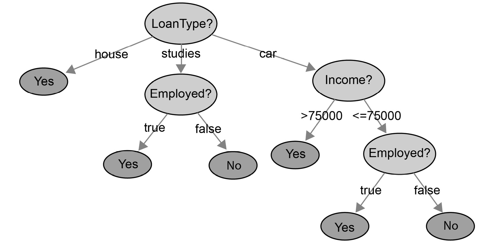
Figure 4.2: Decision tree for the loan type

First, we determine the loan type. House loans are automatically creditworthy according to the first rule. Study loans are described by the second rule, resulting in a subtree containing another decision on employment. Since we have covered both house and study loans, there are only car loans left. The third rule describes an income decision, while the fourth rule describes a decision on employment.

Whenever we must score a new debtor to determine whether they are creditworthy, we have to go through the decision tree from top to bottom and observe the true or false value at the bottom.

Obviously, a model based on seven data points is highly inaccurate because we can't generalize rules that simply do not match reality. Therefore, rules are often determined based on large amounts of data.

This is not the only way that we can create a decision tree. We can build decision trees based on other sequences of rules, too. Let's extract some other rules from the dataset in Figure 4.1.

Observation 1: Notice that individual salaries that are greater than 75,000 are all creditworthy.

Rule 1: Income > 75,000 => CreditWorthy is true.

Rule 1 classifies four out of seven data points (IDs C, E, F, G); we need more rules for the remaining three data points.

Observation 2: Out of the remaining three data points, two are not employed. One is employed (ID D) and is creditworthy. With this, we can claim the following rule:

Rule 2: Assuming Income <= 75,000, the following holds true: Employed == true => CreditWorthy.

Note that with this second rule, we can also classify the remaining two data points (IDs A and B) as not creditworthy. With just two rules, we accurately classified all the observations from this dataset:

Figure 4.3: Decision tree for income

The second decision tree is less complex. At the same time, we cannot overlook the fact that the model says, employed people with a lower income are less likely to pay back their loans. Unfortunately, there is not enough training data available (there are only seven observations in this example), which makes it likely that we'll end up with false conclusions.

Overfitting is a frequent problem in decision trees when making a decision based on a few data points. This decision is rarely representative.

Since we can build decision trees in any possible order, it makes sense to define an efficient way of constructing a decision tree. Therefore, we will now explore a measure for ordering the features in the decision process.

Entropy

In information theory, entropy measures how randomly distributed the possible values of an attribute are. The higher the degree of randomness is, the higher the entropy of the attribute.

Entropy is the highest possibility of an event. If we know beforehand what the outcome will be, then the event has no randomness. So, entropy is zero.

We use entropy to order the splitting of nodes in the decision tree. Taking the previous example, which rule should we start with? Should it be Income <= 75000 or is employed? We need to use a metric that can tell us that one specific split is better than the other. A good split can be defined by the fact it clearly split the data into two homogenous groups. One of these metrics is information gain, and it is based on entropy.

Here is the formula for calculating entropy:

Figure 4.4: Entropy formula

pi represents the probability of one of the possible values of the target variable occurring. So, if this column has n different unique values, then we will have the probability for each of them ([p1, p2, ..., pn]) and apply the formula.

To manually calculate the entropy of a distribution in Python, we can use the np.log2 and np.dot() methods from the NumPy library. There is no function in numpy to automatically calculate entropy.

Have a look at the following example:

import numpy as np

probabilities = list(range(1,4))

minus_probabilities = [-x for x in probabilities]

log_probabilities = [x for x in map(np.log2, probabilities)]

entropy_value = np.dot(minus_probabilities, log_probabilities)

The probabilities are given as a NumPy array or a regular list on line 2: pi.

We need to create a vector of the negated values of the distribution in line 3: - pi.

In line 4, we must take the base two logarithms of each value in the distribution list: logi pi.

Finally, we calculate the sum with the scalar product, also known as the dot product of the two vectors:

Figure 4.5: Dot product of two vectors

Note

You learned about the dot product for the first time in Chapter 2, An Introduction to Regression. The dot product of two vectors is calculated by multiplying the ith coordinate of the first vector by the ith coordinate of the second vector, for each i. Once we have all the products, we sum the values:

np.dot([1, 2, 3], [4, 5, 6])

This results in 1*4 + 2*5 + 3*6 = 32.

In the next exercise, we will be calculating entropy on a small sample dataset.

Exercise 4.01: Calculating Entropy

In this exercise, we will calculate the entropy of the features in the dataset in Figure 4.6:

Figure 4.6: Sample dataset to formulate the rules

Note

The dataset file can also be found in our GitHub repository:

https://packt.live/2AQ6Uo9.

We will calculate entropy for the Employed, Income, LoanType, and LoanAmount features.

The following steps will help you complete this exercise:

1. Open a new Jupyter Notebook file.
2. Import the numpy package as np:

   import numpy as np

3. Define a function called entropy() that receives an array of probabilities and then returns the calculated entropy value, as shown in the following code snippet:

   def entropy(probabilities):

       minus_probabilities = [-x for x in probabilities]

       log_probabilities = [x for x in map(np.log2,

                                           probabilities)]

       return np.dot(minus_probabilities, log_probabilities)

   Next, we will calculate the entropy of the Employed column. This column contains only two possible values: true or false. The true value appeared four times out of seven rows, so its probability is 4/7. Similarly, the probability of the false value is 3/7 as it appeared three times in this dataset.

4. Use the entropy() function to calculate the entropy of the Employed column with the probabilities 4/7 and 3/7:

   H_employed = entropy([4/7, 3/7])

   H_employed

   You should get the following output:

   0.9852281360342515

   This value is quite close to zero, which means the groups are quite homogenous.

5. Now, use the entropy() function to calculate the entropy of the Income column with its corresponding list of probabilities:

   H_income = entropy([1/7, 2/7, 1/7, 2/7, 1/7])

   H_income

   You should get the following output:

   2.2359263506290326

   Compared to the Employed column, the entropy for Income is higher. This means the probabilities of this column are more spread.

6. Use the entropy function to calculate the entropy of the LoanType column with its corresponding list of probabilities:

   H_loanType = entropy([3/7, 2/7, 2/7])

   H_loanType

   You should get the following output:

   1.5566567074628228

   This value is higher than 0, so the probabilities for this column are quite spread.

7. Let's use the entropy function to calculate the entropy of the LoanAmount column with its corresponding list of probabilities:

   H_LoanAmount = entropy([1/7, 1/7, 3/7, 1/7, 1/7])

   H_LoanAmount

   You should get the following output:

   2.128085278891394

   The entropy for LoanAmount is quite high, so its values are quite random.

   Note

   To access the source code for this specific section, please refer to https://packt.live/37T8DVz.

   You can also run this example online at https://packt.live/2By7aI6. You must execute the entire Notebook in order to get the desired result.

Here, you can see that the Employed column has the lowest entropy among the four different columns because it has the least variation in terms of values.

By completing this exercise, you've learned how to manually calculate the entropy for each column of a dataset.

Information Gain

When we partition the data points in a dataset according to the values of an attribute, we reduce the entropy of the system.

To describe information gain, we can calculate the distribution of the labels. Initially, in Figure 4.1, we had five creditworthy and two not creditworthy individuals in our dataset. The entropy belonging to the initial distribution is as follows:

H_label = entropy([5/7, 2/7])

H_label

The output is as follows:

0.863120568566631

Let's see what happens if we partition the dataset based on whether the loan amount is greater than 15,000 or not:

• In group 1, we get one data point belonging to the 15,000 loan amount. This data point is not creditworthy.
• In group 2, we have five creditworthy individuals and one non-creditworthy individual.

The entropy of the labels in each group is as follows.

For group 1, we have the following:

H_group1 = entropy([1])

H_group1

The output is as follows:

-0.0

For group 2, we have the following:

H_group2 = entropy([5/6, 1/6])

H_group2

The output is as follows:

0.6500224216483541

To calculate the information gain, let's calculate the weighted average of the group entropies:

H_group1 * 1/7 + H_group2 * 6/7

The output is as follows:

0.5571620756985892

Now, to find the information gain, we need to calculate the difference between the original entropy (H_label) and the one we just calculated:

Information_gain = 0.863120568566631 - 0.5572

Information_gain

The output is as follows:

0.30592056856663097

By splitting the data with this rule, we gain a little bit of information.

When creating the decision tree, on each node, our job is to partition the dataset using a rule that maximizes the information gain.

We could also use Gini Impurity instead of entropy-based information gain to construct the best rules for splitting decision trees.

Gini Impurity

Instead of entropy, there is another widely used metric that can be used to measure the randomness of a distribution: Gini Impurity.

Gini Impurity is defined as follows:

Figure 4.7: Gini Impurity

pi here represents the probability of one of the possible values of the target variable occurring.

Entropy may be a bit slower to calculate because of the usage of the logarithm. Gini Impurity, on the other hand, is less precise when it comes to measuring randomness.

Note

Some programmers prefer Gini Impurity because you don't have to calculate with logarithms. Computation-wise, none of the solutions are particularly complex, and so both can be used. When it comes to performance, the following study concluded that there are often just minimal differences between the two metrics: https://www.unine.ch/files/live/sites/imi/files/shared/documents/papers/Gini_index_fulltext.pdf.

With this, we have learned that we can optimize a decision tree by splitting the data based on information gain or Gini Impurity. Unfortunately, these metrics are only available for discrete values. What if the label is defined on a continuous interval such as a price range or salary range?

We have to use other metrics. You can technically understand the idea behind creating a decision tree based on a continuous label, which was about regression. One metric we can reuse in this chapter is the mean squared error. Instead of Gini Impurity or information gain, we have to minimize the mean squared error to optimize the decision tree. As this is a beginner's course, we will omit this metric.

In the next section, we will discuss the exit condition for a decision tree.

Exit Condition

We can continuously split the data points according to more and more specific rules until each leaf of the decision tree has an entropy of zero. The question is whether this end state is desirable.

Often, this is not what we expect, because we risk overfitting the model. When our rules for the model are too specific and too nitpicky, and the sample size that the decision was made on is too small, we risk making a false conclusion, thus recognizing a pattern in the dataset that simply does not exist in real life.

For instance, if we spin a roulette wheel three times and we get 12, 25, and 12, this concludes that every odd spin resulting in the value 12 is not a sensible strategy. By assuming that every odd spin equals 12, we find a rule that is exclusively due to random noise.

Therefore, posing a restriction on the minimum size of the dataset that we can still split is an exit condition that works well in practice. For instance, if you stop splitting as soon as you have a dataset that's lower than 50, 100, 200, or 500 in size, you avoid drawing conclusions on random noise, and so you minimize the risk of overfitting the model.

Another popular exit condition is the maximum restriction on the depth of the tree. Once we reach a fixed tree depth, we classify the data points in the leaves.

Building Decision Tree Classifiers Using scikit-learn

We have already learned how to load data from a .csv file, how to apply preprocessing to data, and how to split data into training and testing datasets. If you need to refresh yourself on this knowledge, you can go back to the previous chapters, where you can go through this process in the context of regression and classification.

Now, we will assume that a set of training features, training labels, testing features, and testing labels have been given as a return value of the scikit-learn train-test-split call:

from sklearn import model_selection

features_train, features_test,

label_train, label_test =

model_selection.train_test_split(features, label, test_size=0.1,

                                 random_state=8)

In the preceding code snippet, we used train_test_split to split the dataset (features and labels) into training and testing sets. The testing set represents 10% of the observation (test_size=0.1). The random_state parameter is used to get reproducible results.

We will not focus on how we got these data points because this process is exactly the same as in the case of regression and classification.

It's time to import and use the decision tree classifier of scikit-learn:

from sklearn.tree import DecisionTreeClassifier

decision_tree = DecisionTreeClassifier(max_depth=6)

decision_tree.fit(features_train, label_train)

We set one optional parameter in DecisionTreeClassifier, that is, max_depth, to limit the depth of the decision tree.

Note

You can read the official documentation for the full list of parameters: http://scikit-learn.org/stable/modules/generated/sklearn.tree.DecisionTreeClassifier.html.

Some of the more important parameters are as follows:

• criterion: Gini stands for Gini Impurity, while entropy stands for information gain. This will define which measure will be used to assess the quality of a split at each node.
• max_depth: This is the parameter that defines the maximum depth of the tree.
• min_samples_split: This is the minimum number of samples needed to split an internal node.

You can also experiment with all the other parameters that were enumerated in the documentation. We will omit them in this section.

Once the model has been built, we can use the decision tree classifier to predict data:

decision_tree.predict(features_test)

You will build a decision tree classifier in the activity at the end of this section.

Performance Metrics for Classifiers

After splitting the training and testing data, the decision tree model has a score method to evaluate how well testing data is classified by the model (also known as the accuracy score). We learned how to use the score method in the previous two chapters:

decision_tree.score(features_test, label_test)

The return value of the score method is a number that's less than or equal to 1. The closer we get to 1, the better our model is.

Now, we will learn about another way to evaluate the model.

Note

Feel free to use this method on the models you constructed in the previous chapter as well.

Suppose we have one test feature and one test label:

predicted_label = decision_tree.predict(features_test)

Let's use the previous creditworthy example and assume we trained a decision tree and now have its predictions:

Figure 4.8: Sample dataset to formulate the rules

Our model, in general, made good predictions but had few errors. It incorrectly predicted the results for IDs A, D, and E. Its accuracy score will be 4 / 7 = 0.57.

We will use the following definitions to define some metrics that will help you evaluate how good your classifier is:

• True positive (or TP): All the observations where the true label (the Creditworthy column, in our example) and the corresponding predictions both have the value Yes. In our example, IDs C, F, and G will fall under this category.
• True negative (or TN): All the observations where the true label and the corresponding predictions both have the value No. Only ID B will be classified as true negative.
• False positive (or FP): All the observations where the prediction is Yes but the true label is actually No. This will be the case for ID A.
• False negative (or FN): All the observations where the prediction is No but the true label is actually Yes, such as for IDs D and E.

Using the preceding four definitions, we can define four metrics that describe how well our model predicts the target variable. The #( X ) symbol denotes the number of values in X. Using technical terms, #( X ) denotes the cardinality of X:

Definition (Accuracy): #( True Positives ) + #( True Negatives ) / #( Dataset )

Accuracy is a metric that's used for determining how many times the classifier gives us the correct answer. This is the first metric we used to evaluate the score of a classifier.

In our previous example (Figure 4.8), the accuracy score will be TP + TN / total = (3 + 1) / 7 = 4/7.

We can use the function provided by scikit-learn to calculate the accuracy of a model:

from sklearn.metrics import accuracy_score

accuracy_score(label_test, predicted_label)

Definition (Precision): #TruePositives / (#TruePositives + #FalsePositives)

Precision centers around values that our classifier found to be positive. Some of these results are true positive, while others are false positive. High precision means that the number of false positive results is very low compared to the true positive results. This means that a precise classifier rarely makes a mistake when finding a positive result.

Definition (Recall): #True Positives / (#True Positives + #False Negatives)

Recall centers around values that are positive among the test data. Some of these results are found by the classifier. These are the true positive values. Those positive values that are not found by the classifier are false negatives. A classifier with a high recall value finds most of the positive values.

Using our previous example (Figure 4.8), we will get the following measures:

• Precision = TP / (TP + FP) = 4 / (4 + 1) = 4/6 = 0.8
• Recall = TP / (TP + FN) = 4 / (4 + 2) = 4/6 = 0.6667

With these two measures, we can easily see where our model is performing better or worse. In this example, we know it tends to misclassify false negative cases. These measures are more granular than the accuracy score, which only gives you an overall score.

The F1 score is a metric that combines precision and recall scores. Its value ranges between 0 and 1. If the F1 score equals 1, it means the model is perfectly predicting the right outcomes. On the other hand, an F1 score of 0 means the model cannot predict the target variable accurately. The advantage of the F1 score is that it considers both false positives and false negatives.

The formula for calculating the F1 score is as follows:

Figure 4.9: Formula to calculate the F1 score

As a final note, the scikit-learn package also provides a handy function that can show all these measures in one go: classification_report(). A classification report is useful to check the quality of our predictions:

from sklearn.metrics import classification_report

print(classification_report(label_test, predicted_label))

In the next exercise, we will be practicing how to calculate these scores manually.

Exercise 4.02: Precision, Recall, and F1 Score Calculation

In this exercise, we will calculate the precision, recall value, and the F1 score of two different classifiers on a simulated dataset.

The following steps will help you complete this exercise:

1. Open a new Jupyter Notebook file.
2. Import the numpy package as np using the following code:

   import numpy as np

3. Create a numpy array called real_labels that contains the values [True, True, False, True, True]. This list will represent the true values of the target variable for our simulated dataset. Print its content:

   real_labels = np.array([True, True, False, True, True])

   real_labels

   The expected output will be as follows:

   array([ True, True, False, True, True])

4. Create a numpy array called model_1_preds that contains the values [True, False, False, False, False]. This list will represent the predicted values of the first classifier. Print its content:

   model_1_preds = np.array([True, False, False, False, False])

   model_1_preds

   The expected output will be as follows:

   array([ True, False, False, False, False])

5. Create another numpy array called model_2_preds that contains the values [True, True, True, True, True]. This list will represent the predicted values of the first classifier. Print its content:

   model_2_preds = np.array([True, True, True, True, True])

   model_2_preds

   The expected output will be as follows:

   array([ True, True, True, True, True])

6. Create a variable called model_1_tp_cond that will find the true positives for the first model:

   model_1_tp_cond = (real_labels == True)

                      & (model_1_preds == True)

   model_1_tp_cond

   The expected output will be as follows:

   array([ True, False, False, False, False])

7. Create a variable called model_1_tp that will get the number of true positives for the first model by summing model_1_tp_cond:

   model_1_tp = model_1_tp_cond.sum()

   model_1_tp

   The expected output will be as follows:

   1

   There is only 1 true positive case for the first model.

8. Create a variable called model_1_fp that will get the number of false positives for the first model:

   model_1_fp = ((real_labels == False)

                  & (model_1_preds == True)).sum()

   model_1_fp

   The expected output will be as follows:

   0

   There is no false positive for the first model.

9. Create a variable called model_1_fn that will get the number of false negatives for the first model:

   model_1_fn = ((real_labels == True)

                  & (model_1_preds == False)).sum()

   model_1_fn

   The expected output will be as follows:

   3

   The first classifier presents 3 false negative cases.

10. Create a variable called model_1_precision that will calculate the precision for the first model:

    model_1_precision = model_1_tp / (model_1_tp + model_1_fp)

    model_1_precision

    The expected output will be as follows:

    1.0

    The first classifier has a precision score of 1, so it didn't predict any false positives.

11. Create a variable called model_1_recall that will calculate the recall for the first model:

    model_1_recall = model_1_tp / (model_1_tp + model_1_fn)

    model_1_recall

    The expected output will be as follows:

    0.25

    The recall score for the first model is only 0.25, so it is predicting quite a lot of false negatives.

12. Create a variable called model_1_f1 that will calculate the F1 score for the first model:

    model_1_f1 = 2*model_1_precision * model_1_recall

                 / (model_1_precision + model_1_recall)

    model_1_f1

    The expected output will be as follows:

    0.4

    As expected, the F1 score is quite low for the first model.

13. Create a variable called model_2_tp that will get the number of true positives for the second model:

    model_2_tp = ((real_labels == True)

                   & (model_2_preds == True)).sum()

    model_2_tp

    The expected output will be as follows:

    4

    There are 4 true positive cases for the second model.

14. Create a variable called model_2_fp that will get the number of false positives for the second model:

    model_2_fp = ((real_labels == False)

                   & (model_2_preds == True)).sum()

    model_2_fp

    The expected output will be as follows:

    1

    There is only one false positive for the second model.

15. Create a variable called model_2_fn that will get the number of false negatives for the second model:

    model_2_fn = ((real_labels == True)

                   & (model_2_preds == False)).sum()

    model_2_fn

    The expected output will be as follows:

    0

    There is no false negative for the second classifier.

16. Create a variable called model_2_precision that will calculate precision for the second model:

    model_2_precision = model_2_tp / (model_2_tp + model_2_fp)

    model_2_precision

    The expected output will be as follows:

    0.8

    The precision score for the second model is quite high: 0.8. It is not making too many mistakes regarding false positives.

17. Create a variable called model_2_recall that will calculate recall for the second model:

    model_2_recall = model_2_tp / (model_2_tp + model_2_fn)

    model_2_recall

    The expected output will be as follows:

    1.0

    In terms of recall, the second classifier did a great job and didn't misclassify observations to false negatives.

18. Create a variable called model_2_f1 that will calculate the F1 score for the second model:

    model_2_f1 = 2*model_2_precision*model_2_recall

                 / (model_2_precision + model_2_recall)

    model_2_f1

    The expected output will be as follows:

    0.888888888888889

    The F1 score is quite high for the second model.

    Note

    To access the source code for this specific section, please refer to https://packt.live/3evqbtu.

    You can also run this example online at https://packt.live/2NoxLdo. You must execute the entire Notebook in order to get the desired result.

In this exercise, we saw how to manually calculate the precision, recall, and F1 score for two different models. The first classifier has excellent precision but bad recall, while the second classifier has excellent recall and quite good precision.

Evaluating the Performance of Classifiers with scikit-learn

The scikit-learn package provides some functions for automatically calculating the precision, recall, and F1 score for you. You will need to import them first:

from sklearn.metrics import recall_score,

precision_score, f1_score

To get the precision score, you will need to get the predictions from your model, as shown in the following code snippet:

label_predicted = decision_tree.predict(data)

precision_score(label_test, predicted_label,

                average='weighted')

Calculating the recall_score can be done like so:

recall_score(label_test, label_predicted, average='weighted')

Calculating the f1_score can be done like so:

f1_score(label_test, predicted_label, average='weighted')

In the next section, we will learn how to use another tool, called the confusion matrix, to analyze the performance of a classifier.

The Confusion Matrix

Previously, we learned how to use some calculated metrics to assess the performance of a classifier. There is another very interesting tool that can help you evaluate the performance of a multi-class classification model: the confusion matrix.

A confusion matrix is a square matrix where the number of rows and columns equals the number of distinct label values (or classes). In the columns of the matrix, we place each test label value. In the rows of the matrix, we place each predicted label value.

A confusion matrix looks like this:

Figure 4.10: Sample confusion matrix

In the preceding example, the first row of the confusion matrix is showing us that the model is doing the following:

• Correctly predicting class A 88 times
• Predicting class A when the true value is B 3 times
• Predicting class A when the true value is C 2 times

We can also see the scenario where the model is making a lot of mistakes when it is predicting C while the true value is A (16 times). A confusion matrix is a powerful tool to quickly and easily spot which classes your model is performing well or badly for.

The scikit-learn package provides a function to calculate and display a confusion matrix:

from sklearn.metrics import confusion_matrix

confusion_matrix(label_test, predicted_label)

In the next activity, you will be building a decision tree that will classify cars as unacceptable, acceptable, good, and very good for customers.

Activity 4.01: Car Data Classification

In this activity, you will build a reliable decision tree model that's capable of aiding a company in finding cars that clients are likely to buy. We will be assuming that the car rental agency is focusing on building a lasting relationship with its clients. Your task is to build a decision tree model that classifies cars into one of four categories: unacceptable, acceptable, good, and very good.

Note

The dataset file can also be found in our GitHub repository: https://packt.live/2V95I6h.

The dataset for this activity can be accessed here: https://archive.ics.uci.edu/ml/datasets/Car+Evaluation.

Citation – Dua, D., & Graff, C.. (2017). UCI Machine Learning Repository.

It is composed of six different features: buying, maintenance, doors, persons, luggage_boot, and safety. The target variable ranks the level of acceptability for a given car. It can take four different values: unacc, acc, good, and vgood.

The following steps will help you complete this activity:

1. Load the dataset into Python and import the necessary libaries.
2. Perform label encoding with LabelEncoder() from scikit-learn.
3. Extract the label variable using pop() from pandas.
4. Now, separate the training and testing data with train_test_spit() from scikit-learn. We will use 10% of the data as test data.
5. Build the decision tree classifier using DecisionTreeClassifier() and its methods, fit() and predict().
6. Check the score of our model based on the test data with score().
7. Create a deeper evaluation of the model using classification_report() from scikit-learn.

Expected output:

Figure 4.11: Output showing the expected classification report

Note

The solution to this activity can be found on page 353.

In the next section we will be looking at Random Forest Classifier.

Random Forest Classifier

If you think about the name random forest classifier, it can be explained as follows:

• A forest consists of multiple trees.
• These trees can be used for classification.
• Since the only tree we have used so far for classification is a decision tree, it makes sense that the random forest is a forest of decision trees.
• The random nature of the trees means that our decision trees are constructed in a randomized manner.

Therefore, we will base our decision tree construction on information gain or Gini Impurity.

Once you understand these basic concepts, you essentially know what a random forest classifier is all about. The more trees you have in the forest, the more accurate prediction is going to be. When performing prediction, each tree performs classification. We collect the results, and the class that gets the most votes wins.

Random forests can be used for regression as well as for classification. When using random forests for regression, instead of counting the most votes for a class, we take the average of the arithmetic mean (average) of the prediction results and return it. Random forests are not as ideal for regression as they are for classification, though, because the models that are used to predict values are often out of control, and often return a wide range of values. The average of these values is often not too meaningful. Managing the noise in a regression exercise is harder than in classification.

Random forests are often better than one simple decision tree because they provide redundancy. They treat outlier values better and have a lower probability of overfitting the model. Decision trees seem to behave great as long as you are using them on the data that was used when creating the model. Once you use them to predict new data, random forests lose their edge. Random forests are widely used for classification problems, whether it be customer segmentation for banks or e-commerce, classifying images, or medicine. If you own an Xbox with Kinect, your Kinect device contains a random forest classifier to detect your body.

Random forest is an ensemble algorithm. The idea behind ensemble learning is that we take an aggregated view of a decision of multiple agents that potentially have different weaknesses. Due to the aggregated vote, these weaknesses cancel out, and the majority vote likely represents the correct result.

Random Forest Classification Using scikit-learn

As you may have guessed, the scikit-learn package provides an implementation of the RandomForest classifier with the RandomForestClassifier class. This class provides the exact same methods as all the scikit-learn models you have seen so far – you need to instantiate a model, then fit it with the training set with .fit(), and finally make predictions with .predict():

from sklearn.ensemble import RandomForestClassifier

random_forest_classifier = RandomForestClassifier()

random_forest_classifier.fit(features_train, label_train)

labels_predicted = random_forest_classifier.predict

                   (features_test)

In the next section, we will be looking at the parameterization of the random forest classifier.

The Parameterization of the Random Forest Classifier

We will be considering a subset of the possible parameters, based on what we already know, which is based on the description of constructing random forests:

• n_estimators: The number of trees in the random forest. The default value is 10.
• criterion: Use Gini or entropy to determine whether you use Gini Impurity or information gain using the entropy in each tree. This will be used to find the best split at each node.
• max_features: The maximum number of features considered in any tree of the forest. Possible values include an integer. You can also add some strings such as sqrt for the square root of the number of features.
• max_depth: The maximum depth of each tree.
• min_samples_split: The minimum number of samples in the dataset in a given node to perform a split. This may also reduce the tree's size.
• bootstrap: A Boolean that indicates whether to use bootstrapping on data points when constructing trees.

Feature Importance

A random forest classifier gives you information on how important each feature in the data classification process is. Remember, we used a lot of randomly constructed decision trees to classify data points. We can measure how accurately these data points behave, and we can also see which features are vital when it comes to decision-making.

We can retrieve the array of feature importance scores with the following query:

random_forest_classifier.feature_importances_

In this six-feature classifier, the fourth and sixth features are clearly a lot more important than any other features. The third feature has a very low importance score.

Feature importance scores come in handy when we have a lot of features and we want to reduce the feature size to avoid the classifier getting lost in the details. When we have a lot of features, we risk overfitting the model. Therefore, reducing the number of features by dropping the least significant ones is often helpful.

Cross-Validation

Earlier, we learned how to use different metrics to assess the performance of a classifier, such as the accuracy, precision, recall, or the F1 score on a training and testing set. The objective is to have a high score on both sets that are very close to each other. In that case, your model is performant and not prone to overfitting.

The test set is used as a proxy to evaluate whether your model can generalize well to unseen data or whether it learns patterns that are only relevant to the training set.

But in the case of having quite a few hyperparameters to tune (such as for RandomForest), you will have to train a lot of different models and test them on your testing set. This kind of defeats the purpose of the testing set. Think of the testing set as the final exam that will define whether you pass a subject or not. You will not be allowed to pass and repass it over and over.

One solution for avoiding using the testing set too much is creating a validation set. You will train your model on the training set and use the validation set to assess its score according to different combinations of hyperparameters. Once you find your best model, you will use the testing set to make sure it doesn't overfit too much. This is, in general, the suggested approach for any data science project.

The drawback of this approach is that you are reducing the number of observations for the training set. If you have a dataset with millions of rows, it is not a problem. But for a small dataset, this can be problematic. This is where cross-validation comes in.

The following Figure 4.12, shows that this is a technique where you create multiple splits of the training data. For each split, the training data is separated into folds (five, in this example) and one of the folds will be used as the validation set while the others will be used for training.

For instance, for the top split, fold 5 will be used for validation and the four other folds (1 to 4) will be used to train the model. You will follow the same process for each split. After going through each split, you will have used the entire training data and the final performance score will be the average of all the models that were trained on each split:

Figure 4.12: Cross-validation example

With scikit-learn, you can easily perform cross-validation, as shown in the following code snippet:

from sklearn.ensemble import RandomForestClassifier

random_forest_classifier = RandomForestClassifier()

from sklearn.model_selection import cross_val_score

cross_val_score(random_forest_classifier, features_train,

                label_train, cv=5, scoring='accuracy')

cross_val_score takes two parameters:

• cv: Specifies the number of splits.
• scoring: Defines which performance metrics you want to use. You can find the list of possible values here: https://scikit-learn.org/stable/modules/model_evaluation.html#scoring-parameter.

In the next section, we will look at a specific variant of RandomForest, called extratrees.

Extremely Randomized Trees

Extremely randomized trees increase the randomization inside random forests by randomizing the splitting rules on top of the already randomized factors in random forests.

Parameterization is like the random forest classifier. You can see the full list of parameters here: http://scikit-learn.org/stable/modules/generated/sklearn.ensemble.ExtraTreesClassifier.html.

The Python implementation is as follows:

from sklearn.ensemble import ExtraTreesClassifier

extra_trees_classifier =

ExtraTreesClassifier(n_estimators=100,

                     max_depth=6)

extra_trees_classifier.fit(features_train, label_train)

labels_predicted = extra_trees_classifier.predict(features_test)

In the following activity, we will be optimizing the classifier built in Activity 4.01, Car Data Classification.

Activity 4.02: Random Forest Classification for Your Car Rental Company

In this activity, you will optimize your classifier so that you satisfy your clients more when selecting future cars for your car fleet. We will be performing random forest and extreme random forest classification on the car dealership dataset that you worked on in the previous activity of this chapter.

The following steps will help you complete this activity:

1. Follow Steps 1 - 4 of the previous Activity 4.01, Car Data Classification.
2. Create a random forest using RandomForestClassifier.
3. Train the models using .fit().
4. Import the confusion_matrix function to find the quality of the RandomForest.
5. Print the classification report using classification_report().
6. Print the feature importance with .feature_importance_.
7. Repeat Steps 2 to 6 with an extratrees model.

Expected output:

array([0.08844544, 0.0702334 , 0.01440408, 0.37662014,

       0.05965896, 0.39063797])

Note

The solution to this activity can be found on page 357.

By completing this activity, you've learned how to fit the RandomForest and extratrees models and analyze their classification report and feature importance. Now, you can try different hyperparameters on your own and see if you can improve their results.

Summary

In this chapter, we learned how to use decision trees for prediction. Using ensemble learning techniques, we created complex reinforcement learning models to predict the class of an arbitrary data point.

Decision trees proved to be very accurate on the surface, but they were prone to overfitting the model. Random forests and extremely randomized trees reduce overfitting by introducing some random elements and a voting algorithm, where the majority wins.

Beyond decision trees, random forests, and extremely randomized trees, we also learned about new methods for evaluating the utility of a model. After using the well-known accuracy score, we started using the precision, recall, and F1 score metrics to evaluate how well our classifier works. All of these values were derived from the confusion matrix.

In the next chapter, we will describe the clustering problem and compare and contrast two clustering algorithms.