6. Neural Networks and Deep Learning

Overview

In this chapter, you will be introduced to the final topic on neural networks and deep learning. You will be learning about TensorFlow, Convolutional Neural Networks (CNNs), and Recurrent Neural Networks (RNNs). You will use key deep learning concepts to determine creditworthiness of individuals and predict housing prices in a neighborhood. Later on, you will also implement an image classification program using the skills you learned. By the end of this chapter, you will have a firm grasp on the concepts of neural networks and deep learning.

Introduction

In the previous chapter, we learned about what clustering problems are and saw several algorithms, such as k-means, that can automatically group data points on their own. In this chapter, we will learn about neural networks and deep learning networks.

The difference between neural networks and deep learning networks is the complexity and depth of the networks. Traditionally, neural networks have only one hidden layer, while deep learning networks have more than that.

Although we will use neural networks and deep learning for supervised learning, note that neural networks can also model unsupervised learning techniques. This kind of model was actually quite popular in the 1980s, but because the computation power required was limited at the time, it's only recently that this model has been widely adopted. With the democratization of Graphics Processing Units (GPUs) and cloud computing, we now have access to a tremendous amount of computation power. This is the main reason why neural networks and especially deep learning are hot topics again.

Deep learning can model more complex patterns than traditional neural networks, and so deep learning is more widely used nowadays in computer vision (in applications such as face detection and image recognition) and natural language processing (in applications such as chatbots and text generation).

Artificial Neurons

Artificial Neural Networks (ANNs), as the name implies, try to replicate how a human brain works, and more specifically how neurons work.

A neuron is a cell in the brain that communicates with other cells via electrical signals. Neurons can respond to stimuli such as sound, light, and touch. They can also trigger actions such as muscle contractions. On average, a human brain contains 10 to 20 billion neurons. That's a pretty huge network, right? This is the reason why humans can achieve so many amazing things. This is also why researchers have tried to emulate how the brain operates and in doing so created ANNs.

ANNs are composed of multiple artificial neurons that connect to each other and form a network. An artificial neuron is simply a processing unit that performs mathematical operations on some inputs (x1, x2, …, xn) and returns the final results (y) to the next unit, as shown here:

Figure 6.1: Representation of an artificial neuron

We will see how an artificial neuron works more in detail in the coming sections.

Neurons in TensorFlow

TensorFlow is currently the most popular neural network and deep learning framework. It was created and is maintained by Google. TensorFlow is used for voice recognition and voice search, and it is also the brain behind translate.google.com. Later in this chapter, we will use TensorFlow to recognize written characters.

The TensorFlow API is available in many languages, including Python, JavaScript, Java, and C. TensorFlow works with tensors. You can think of a tensor as a container composed of a matrix (usually with high dimensions) and additional information related to the operations it will perform (such as weights and biases, which you will be looking at later in this chapter). A tensor with no dimensions (with no rank) is a scalar. A tensor of rank 1 is a vector, rank 2 tensors are matrices, and a rank 3 tensor is a three-dimensional matrix. The rank indicates the dimensions of a tensor. In this chapter, we will be looking at tensors of ranks 2 and 3.

Note

Mathematicians use the terms matrix and dimension, whereas deep learning programmers use tensor and rank instead.

TensorFlow also comes with mathematical functions to transform tensors, such as the following:

• Arithmetic operations: add and multiply
• Exponential operations: exp and log
• Relational operations: greater, less, and equal
• Array operations: concat, slice, and split
• Matrix operations: matrix_inverse, matrix_determinant, and matmul
• Non-linear operations: sigmoid, relu, and softmax

We will go through them in more detail later in this chapter.

In the next exercise, we will be using TensorFlow to compute an artificial neuron.

Exercise 6.01: Using Basic Operations and TensorFlow Constants

In this exercise, we will be using arithmetic operations in TensorFlow to emulate an artificial neuron by performing a matrix multiplication and addition, and applying a non-linear function, sigmoid.

The following steps will help you complete the exercise:

1. Open a new Jupyter Notebook file.
2. Import the tensorflow package as tf:

   import tensorflow as tf

3. Create a tensor called W of shape [1,6] (that is, with 1 row and 6 columns), using tf.constant(), that contains the matrix [1.0, 2.0, 3.0, 4.0, 5.0, 6.0]. Print its value:

   W = tf.constant([1.0, 2.0, 3.0, 4.0, 5.0, 6.0], shape=[1, 6])

   W

   The expected output is this:

   <tf.Tensor: shape=(1, 6), dtype=float32, numpy=array([[1., 2., 3., 4., 5., 6.]], dtype=float32)>

4. Create a tensor called X of shape [6,1] (that is, with 6 rows and 1 column), using tf.constant(), that contains [7.0, 8.0, 9.0, 10.0, 11.0, 12.0]. Print its value:

   X = tf.constant([7.0, 8.0, 9.0, 10.0, 11.0, 12.0],

                   shape=[6, 1])

   X

   The expected output is this:

   <tf.Tensor: shape=(6, 1), dtype=float32, numpy=

   array([[ 7.],

          [ 8.],

          [ 9.],

          [10.],

          [11.],

          [12.]], dtype=float32)>

5. Now, create a tensor called b, using tf.constant(), that contains -88. Print its value:

   b = tf.constant(-88.0)

   b

   The expected output is this:

   <tf.Tensor: shape=(), dtype=float32, numpy=-88.0>

6. Perform a matrix multiplication between W and X using tf.matmul, save its results in the mult variable, and print its value:

   mult = tf.matmul(W, X)

   mult

   The expected output is this:

   <tf.Tensor: shape=(1, 1), dtype=float32, numpy=array([[217.]], dtype=float32)>

7. Perform a matrix addition between mult and b, save its results in a variable called Z, and print its value:

   Z = mult + b

   Z

   The expected output is this:

   <tf.Tensor: shape=(1, 1), dtype=float32, numpy=array([[129.]], dtype=float32)>

8. Apply the sigmoid function to Z using tf.math.sigmoid, save its results in a variable called a, and print its value. The sigmoid function transforms any numerical value within the range 0 to 1 (we will learn more about this in the following sections):

   a = tf.math.sigmoid(Z)

   a

   The expected output is this:

   <tf.Tensor: shape=(1, 1), dtype=float32, numpy=array([[1.]], dtype=float32)>

The sigmoid function has transformed the original value of Z, which was 129, to 1.

Note

To access the source code for this specific section, please refer to https://packt.live/31ekGLM.

You can also run this example online at https://packt.live/3evuKnC. You must execute the entire Notebook in order to get the desired result.

In this exercise, you successfully implemented an artificial neuron using TensorFlow. This is the base of any neural network model.

In the next section, we will be looking at the architecture of neural networks.

Neural Network Architecture

Neural networks are the newest branch of Artificial Intelligence (AI). Neural networks are inspired by how the human brain works. They were invented in the 1940s by Warren McCulloch and Walter Pitts. The neural network was a mathematical model that was used to describe how the human brain can solve problems.

We will use ANN to refer to both the mathematical model, and the biological neural network when talking about the human brain.

The way a neural network learns is more complex compared to other classification or regression models. The neural network model has a lot of internal variables, and the relationship between the input and output variables may involve multiple internal layers. Neural networks have higher accuracy than other supervised learning algorithms.

Note

Mastering neural networks with TensorFlow is a complex process. The purpose of this section is to provide you with an introductory resource to get started.

In this chapter, the main example we are going to use is the recognition of digits from an image. We are considering this format since each image is small, and we have around 70,000 images available. The processing power required to process these images is similar to that of a regular computer.

ANNs work similarly to how the human brain works. A dendroid in a human brain is connected to a nucleus, and the nucleus is connected to an axon. In an ANN, the input is the dendroid, where the calculations occur is the nucleus, and the output is the axon.

An artificial neuron is designed to replicate how a nucleus works. It will transform an input signal by calculating a matrix multiplication followed by an activation function. If this function determines that a neuron has to fire, a signal appears in the output. This signal can be the input of other neurons in the network:

Figure 6.2: Figure showing how an ANN works

Let's understand the preceding figure further by taking the example of n=4. In this case, the following applies:

• X is the input matrix, which is composed of x1, x2, x3, and x4.
• W, the weight matrix, will be composed of w1, w2, w3, and w4.
• b is the bias.
• f is the activation function.

We will first calculate Z (the left-hand side of the neuron) with matrix multiplication and bias:

Z = W * X + b = x1*w1 + x2*w2 + x3*w3 + x4*w4 + b

Then the output, y, will be calculated by applying a function, f:

y = f(Z) = f(x1*w1 + x2*w2 + x3*w3 + x4*w4 + b)

Great – this is how an artificial neuron works under the hood. It is two matrix operations, a product followed by a sum, and a function transformation.

We now move on to the next section – weights.

Weights

W (also called the weight matrix) refers to weights, which are parameters that are automatically learned by neural networks in order to predict accurately the output, y.

A single neuron is the combination of the weighted sum and the activation function and can be referred to as a hidden layer. A neural network with one hidden layer is called a regular neural network:

Figure 6.3: Neurons 1, 2, and 3 form the hidden layer of this sample network

When connecting inputs and outputs, we may have multiple hidden layers. A neural network with multiple layers is called a deep neural network.

The term deep learning comes from the presence of multiple layers. When creating an Artificial Neural Network (ANN), we can specify the number of hidden layers.

Biases

Previously, we saw that the equation for a neuron is as follows:

y = f(x1*w1 + x2*w2 + x3*w3 + x4*w4)

The problem with this equation is that there is no constant factor that depends on the inputs x1, x2, x3, and x4. The preceding equation can model any linear function that will go through the point 0: if all w values are equal to 0 then y will also equal to 0. But what about other functions that don't go through the point 0? For example, imagine that we are predicting the probability of churn for an employee by their month of tenure. Even if they haven't worked for the full month yet, the probability of churn is not zero.

To accommodate this situation, we need to introduce a new parameter called bias. It is a constant that is also referred to as the intercept. Using the churn example, the bias b can equal to 0.5 and therefore the churn probability for a new employer during the first month will be 50%.

Therefore, we add bias to the equation:

y = f(x1*w1 + x2*w2 + x3*w3 + x4*w4 + b)

y = f(x w + b)

The first equation is the verbose form, describing the role of each coordinate, weight coefficient, and bias. The second equation is the vector form, where x = (x1, x2, x3, x4) and w = (w1, w2, w3, w4). The dot operator between the vectors symbolizes the dot or scalar product of the two vectors. The two equations are equivalent. We will use the second form in practice because it is easier to define a vector of variables using TensorFlow than to define each variable one by one.

Similarly, for w1, w2, w3, and w4, the bias, b, is a variable, meaning that its value can change during the learning process.

With this constant factor built into each neuron, a neural network model becomes more flexible in terms of fitting a specific training dataset better.

Note

It may happen that the product p = x1*w1 + x2*w2 + x3*w3 + x4*w4 is negative due to the presence of a few negative weights. We may still want to give the model the flexibility to execute (or fire) a neuron with values above a given negative number. Therefore, adding a constant bias, b = 5, for instance, can ensure that the neuron fires for values between -5 and 0 as well.

TensorFlow provides the Dense() class to model the hidden layer of a neural network (also called the fully connected layer):

from tensorflow.keras import layers

layer1 = layers.Dense(units=128, input_shape=[200])

In this example, we have created a fully connected layer of 128 neurons that takes as input a tensor of shape 200.

Note

You can find more information on this TensorFlow class at https://www.tensorflow.org/api_docs/python/tf/keras/layers/Dense.

The Dense() class is expected to have a flattened input (only one row). For instance, if your input is of shape 28 by 28, you will have to flatten it beforehand with the Flatten() class in order to get a single row with 784 neurons (28 * 28):

from tensorflow.keras import layers

input_layer = layers.Flatten(input_shape=(28, 28))

layer1 = layers.Dense(units=128)

Note

You can find more information on this TensorFlow class at https://www.tensorflow.org/api_docs/python/tf/keras/layers/Flatten.

In the following sections, we will learn about how we can extend this layer of neurons with additional parameters.

Use Cases for ANNs

ANNs have their place among supervised learning techniques. They can model both classification and regression problems. A classifier neural network seeks a relationship between features and labels. The features are the input variables, while each class the classifier can choose as a return value is a separate output. In the case of regression, the input variables are the features, while there is one single output: the predicted value. While traditional classification and regression techniques have their use cases in AI, ANNs are generally better at finding complex relationships between inputs and outputs.

In the next section, we will be looking at activation functions and their different types.

Activation Functions

As seen previously, a single neuron needs to perform a transformation by applying an activation function. Different activation functions can be used in neural networks. Without these functions, a neural network would simply be a linear model that could easily be described using matrix multiplication.

The activation function of a neural network provides non-linearity and therefore can model more complex patterns. Two very common activation functions are sigmoid and tanh (the hyperbolic tangent function).

Sigmoid

The formula of sigmoid is as follows:

Figure 6.4: The sigmoid formula

The output values of a sigmoid function range from 0 to 1. This activation function is usually used at the last layer of a neural network for a binary classification problem.

Tanh

The formula of the hyperbolic tangent is as follows:

Figure 6.5: The tanh formula

The tanh activation function is very similar to the sigmoid function and was quite popular until recently. It is usually used in the hidden layers of a neural network. Its values range between -1 and 1.

ReLU

Another important activation function is relu. ReLU stands for Rectified Linear Unit. It is currently the most widely used activation function for hidden layers. Its formula is as follows:

Figure 6.6: The ReLU formula

There are now different variants of relu functions, such as leaky ReLU and PReLU.

Softmax

The function shrinks the values of a list to be between 0 and 1 so that the sum of the elements of the list becomes 1. The definition of the softmax function is as follows:

Figure 6.7: The softmax formula

The softmax function is usually used as the last layer of a neural network for multi-class classification problems as it can generate probabilities for each of the different output classes.

Remember, in TensorFlow, we can extend a Dense() layer with an activation function; we just need to set the activation parameter. In the following example, we will add the relu activation function:

from tensorflow.keras import layers

layer1 = layers.Dense(units=128, input_shape=[200],

                      activation='relu')

Let's use these different activation functions and observe how these functions dampen the weighted inputs by solving the following exercise.

Exercise 6.02: Activation Functions

In this exercise, we will be implementing the following activation functions using the numpy package: sigmoid, tanh, relu, and softmax.

The following steps will help you complete the exercise:

1. Open a new Jupyter Notebook file.
2. Import the numpy package as np:

   import numpy as np

3. Create a sigmoid function, as shown in the following code snippet, that implements the sigmoid formula (shown in the previous section) using the np.exp() method:

   def sigmoid(x):

       return 1 / (1 + np.exp(-x))

4. Calculate the result of sigmoid function on the value -1:

   sigmoid(-1)

   The expected output is this:

   0.2689414213699951

   This is the result of performing a sigmoid transformation on the value -1.

5. Import the matplotlib.pyplot package as plt:

   import matplotlib.pyplot as plt

6. Create a numpy array called x that contains values from -10 to 10 evenly spaced by an increment of 0.1, using the np.arange() method. Print its value:

   x = np.arange(-10, 10, 0.1)

   x

   The expected output is this:

   array([-1.00000000e+01, -9.90000000e+00, -9.80000000e+00,

          -9.70000000e+00, -9.60000000e+00, -9.50000000e+00,

          -9.40000000e+00, -9.30000000e+00, -9.20000000e+00,

          -9.10000000e+00, -9.00000000e+00, -8.90000000e+00,

          -8.80000000e+00, -8.70000000e+00, -8.60000000e+00,

          -8.50000000e+00, -8.40000000e+00, -8.30000000e+00,

          -8.20000000e+00, -8.10000000e+00, -8.00000000e+00,

          -7.90000000e+00, -7.80000000e+00, -7.70000000e+00,

          -7.60000000e+00, -7.50000000e+00, -7.40000000e+00,

          -7.30000000e+00, -7.20000000e+00, -7.10000000e+00,

          -7.00000000e+00, -6.90000000e+00,

   Great – we generated a numpy array containing values between -10 and 10.

   Note

   The preceding output is truncated.

7. Plot a line chart with x and sigmoid(x) using plt.plot() and plt.show():

   plt.plot(x, sigmoid(x))

   plt.show()

   The expected output is this:

   

   Figure 6.8: Line chart using the sigmoid function

   We can see here that the output of the sigmoid function ranges between 0 and 1. The slope is quite steep for values around 0.

8. Create a tanh() function that implements the Tanh formula (shown in the previous section) using the np.exp() method:

   def tanh(x):

       return 2 / (1 + np.exp(-2*x)) - 1

9. Plot a line chart with x and tanh(x) using plt.plot() and plt.show():

   plt.plot(x, tanh(x))

   plt.show()

   The expected output is this:

   

   Figure 6.9: Line chart using the tanh function

   The shape of the tanh function is very similar to sigmoid but its slope is steeper for values close to 0. Remember, its range is between -1 and 1.

10. Create a relu function that implements the ReLU formula (shown in the previous section) using the np.maximum() method:

    def relu(x):

        return np.maximum(0, x)

11. Plot a line chart with x and relu(x) using plt.plot() and plt.show():

    plt.plot(x, relu(x))

    plt.show()

    The expected output is this:

    

    Figure 6.10: Line chart using the relu function

    The ReLU function equals 0 when values are negative, and equals the identity function, f(x)=x, for positive values.

12. Create a softmax function that implements the softmax formula (shown in the previous section) using the np.exp() method:

    def softmax(list):

        return np.exp(list) / np.sum(np.exp(list))

13. Calculate the output of softmax on the list of values, [0, 1, 168, 8, 2]:

    result = softmax( [0, 1, 168, 8, 2])

    result

    The expected output is this:

    array([1.09276566e-73, 2.97044505e-73, 1.00000000e+00,

           3.25748853e-70, 8.07450679e-73])

As expected, the item at the third position has the highest softmax probabilities as its original value was the highest.

Note

To access the source code for this specific section, please refer to https://packt.live/3fJzoOU.

You can also run this example online at https://packt.live/3188pZi. You must execute the entire Notebook in order to get the desired result.

By completing this exercise, we have implemented some of the most important activation functions for neural networks.

Forward Propagation and the Loss Function

So far, we have seen how a neuron can take an input and perform some mathematical operations on it and get an output. We learned that a neural network is a combination of multiple layers of neurons.

The process of transforming the inputs of a neural network into a result is called forward propagation (or the forward pass). What we are asking the neural network to do is to make a prediction (the final output of the neural network) by applying multiple neurons to the input data:

Figure 6.11: Figure showing forward propagation

The neural network relies on the weights matrices, biases, and activation function of each neuron to calculate the predicted output value, . For now, let's assume the values of the weight matrices and biases are set in advance. The activation functions are defined when you design the architecture of the neural networks.

As for any supervised machine learning algorithm, the goal is to make accurate predictions. This implies that we need to assess how accurate the predictions are compared to the true values. For traditional machine learning algorithms, we used scoring metrics such as mean squared error, accuracy, or the F1 score. This can also be applied to neural networks, but the only difference is that such scores are used in two different ways:

• They are used by data scientists to assess the performance of a model on training and testing sets and then tune hyperparameters if needed. This also applies to neural networks, so nothing new here.
• They are used by neural networks to automatically learn from mistakes and update weight matrices and biases. This will be explained in more detail in the next section, which is about backpropagation. So, the neural network will use a metric (also called a loss function) to compare its predicted values, to the true label, (y), and then learn how to make better predictions automatically.

The loss function is critical to a neural network learning to make good predictions. This is a hyperparameter that needs to be defined by data scientists while designing the architecture of a neural network. The choice of which loss function to use is totally arbitrary and depending on the dataset or the problem you want to solve, you will pick one or another. Luckily for us, though, there are some basic rules of thumb that work in most cases:

• If you are working on a regression problem, you can use mean squared error.
• If it is a binary classification, the loss function should be binary cross-entropy.
• If it is a multi-class classification, then categorical cross-entropy should be your go-to choice.

As a final note, the choice of loss function will also define which activation function you will have to use on the last layer of the neural network. Each loss function expects a certain type of data in order to properly assess prediction performance.

Here is the list of activation functions according to the loss function and type of project/problem:

Figure 6.12: Overview of the different activation functions and their applications

With TensorFlow, in order to build your custom architecture, you can instantiate the Sequential() class and add your layers of fully connected neurons as shown in the following code snippet:

import tensorflow as tf

from tensorflow.keras import layers

model = tf.keras.Sequential()

input_layer = layers.Flatten(input_shape=(28,28))

layer1 = layers.Dense(128, activation='relu')

model.add(input_layer)

model.add(layer1)

Now it is time to have a look at how a neural network improves its predictions with backpropagation.

Backpropagation

Previously, we learned how a neural network makes predictions by using weight matrices and biases (we can combine them into a single matrix) from its neurons. Using the loss function, a network determines how good or bad the predictions are. It would be great if it could use this information and update the parameters accordingly. This is exactly what backpropagation is about: optimizing a neural network's parameters.

Training a neural network involves executing forward propagation and backpropagation multiple times in order to make predictions and update the parameters from the errors. During the first pass (or propagation), we start by initializing all the weights of the neural network. Then, we apply forward propagation, followed by backpropagation, which updates the weights.

We apply this process several times and the neural network will optimize its parameters iteratively. You can decide to stop this learning process by setting the maximum number of times the neural networks will go through the entire dataset (also called epochs) or define an early stop threshold if the neural network's score is not improving anymore after few epochs.

Optimizers and the Learning Rate

In the previous section, we saw that a neural network follows an iterative process to find the best solution for any input dataset. Its learning process is an optimization process. You can use different optimization algorithms (also called optimizers) for a neural network. The most popular ones are Adam, SGD, and RMSprop.

One important parameter for the neural networks optimizer is the learning rate. This value defines how quickly the neural network will update its weights. Defining a too-low learning rate will slow down the learning process and the neural network will take a long time before finding the right parameters. On the other hand, having too-high a learning rate can make the neural network not learn a solution as it is making bigger weight changes than required. A good practice is to start with a not-too-small learning rate (such as 0.01 or 0.001), then stop the neural network training once its score starts to plateau or get worse, and lower the learning rate (by an order of magnitude, for instance) and keep training the network.

With TensorFlow, you can instantiate an optimizer from tf.keras.optimizers. For instance, the following code snippet shows us how to create an Adam optimizer with 0.001 as the learning rate and then compile our neural network by specifying the loss function ('sparse_categorical_crossentropy') and metrics to be displayed ('accuracy'):

import tensorflow as tf

optimizer = tf.keras.optimizers.Adam(0.001)

model.compile(loss='sparse_categorical_crossentropy',

              optimizer=optimizer, metrics=['accuracy'])

Once the model is compiled, we can then train the neural network with the .fit() method like this:

model.fit(features_train, label_train, epochs=5)

Here we trained the neural network on the training set for 5 epochs. Once trained, we can use the model on the testing set and assess its performance with the .evaluate() method:

model.evaluate(features_test, label_test)

Note

You can find more information on this TensorFlow optimizers at https://www.tensorflow.org/api_docs/python/tf/keras/optimizers.

In the next exercise, we will be training a neural network on a dataset.

Exercise 6.03: Classifying Credit Approval

In this exercise, we will be using the German credit approval dataset, and train a neural network to classify whether an individual is creditworthy or not.

Note

The dataset file can also be found in our GitHub repository:

https://packt.live/2V7uiV5.

The following steps will help you complete the exercise:

1. Open a new Jupyter Notebook file.
2. Import the loadtxt method from numpy:

   from numpy import loadtxt

3. Create a variable called file_url containing the link to the raw dataset:

   file_url = 'https://raw.githubusercontent.com/'

              'PacktWorkshops/'

              'The-Applied-Artificial-Intelligence-Workshop'

              '/master/Datasets/german_scaled.csv'

4. Load the data into a variable called data using loadtxt() and specify the delimiter=',' parameter. Print its content:

   data = loadtxt(file_url, delimiter=',')

   data

   The expected output is this:

   array([[0. , 0.33333333, 0.02941176, ..., 0. , 1. ,

           1. ],

          [1. , 0. , 0.64705882, ..., 0. , 0. ,

           1. ],

          [0. , 1. , 0.11764706, ..., 1. , 0. ,

           1. ],

          ...,

          [0. , 1. , 0.11764706, ..., 0. , 0. ,

           1. ],

          [1. , 0.33333333, 0.60294118, ..., 0. , 1. ,

           1. ],

          [0. , 0. , 0.60294118, ..., 0. , 0. ,

           1. ]])

5. Create a variable called label that contains the data only from the first column (this will be our response variable):

   label = data[:, 0]

6. Create a variable called features that contains all the data except for the first column (which corresponds to the response variable):

   features = data[:, 1:]

7. Import the train_test_split method from sklearn.model_selection:

   from sklearn.model_selection import train_test_split

8. Split the data into training and testing sets and save the results into four variables called features_train, features_test, label_train, and label_test. Use 20% of the data for testing and specify random_state=7:

   features_train, features_test,

   label_train, label_test = train_test_split(features,

                                              label,

                                              test_size=0.2,

                                              random_state=7)

9. Import numpy as np, tensorflow as tf, and layers from tensorflow.keras:

   import numpy as np

   import tensorflow as tf

   from tensorflow.keras import layers

10. Set 1 as the seed for numpy and tensorflow using np.random_seed() and tf.random.set_seed():

    np.random.seed(1)

    tf.random.set_seed(1)

11. Instantantiate a tf.keras.Sequential() class and save it into a variable called model:

    model = tf.keras.Sequential()

12. Instantantiate a layers.Dense() class with 16 neurons, activation='relu', and input_shape=[19], then save it into a variable called layer1:

    layer1 = layers.Dense(16, activation='relu',

                          input_shape=[19])

13. Instantantiate a second layers.Dense() class with 1 neuron and activation='sigmoid', then save it into a variable called final_layer:

    final_layer = layers.Dense(1, activation='sigmoid')

14. Add the two layers you just defined to the model using .add():

    model.add(layer1)

    model.add(final_layer)

15. Instantantiate a tf.keras.optimizers.Adam() class with 0.001 as the learning rate and save it into a variable called optimizer:

    optimizer = tf.keras.optimizers.Adam(0.001)

16. Compile the neural network using .compile() with loss='binary_crossentropy', optimizer=optimizer, metrics=['accuracy'] as shown in the following code snippet:

    model.compile(loss='binary_crossentropy',

                  optimizer=optimizer, metrics=['accuracy'])

17. Print a summary of the model using .summary():

    model.summary()

    The expected output is this:

    

    Figure 6.13: Summary of the sequential model

    This output summarizes the architecture of our neural networks. We can see it is composed of three layers, as expected, and we know each layer's output size and number of parameters, which corresponds to the weights and biases. For instance, the first layer has 16 neurons and 320 parameters to be learned (weights and biases).

18. Next, fit the neural networks with the training set and specify epochs=10:

    model.fit(features_train, label_train, epochs=10)

    The expected output is this:

    

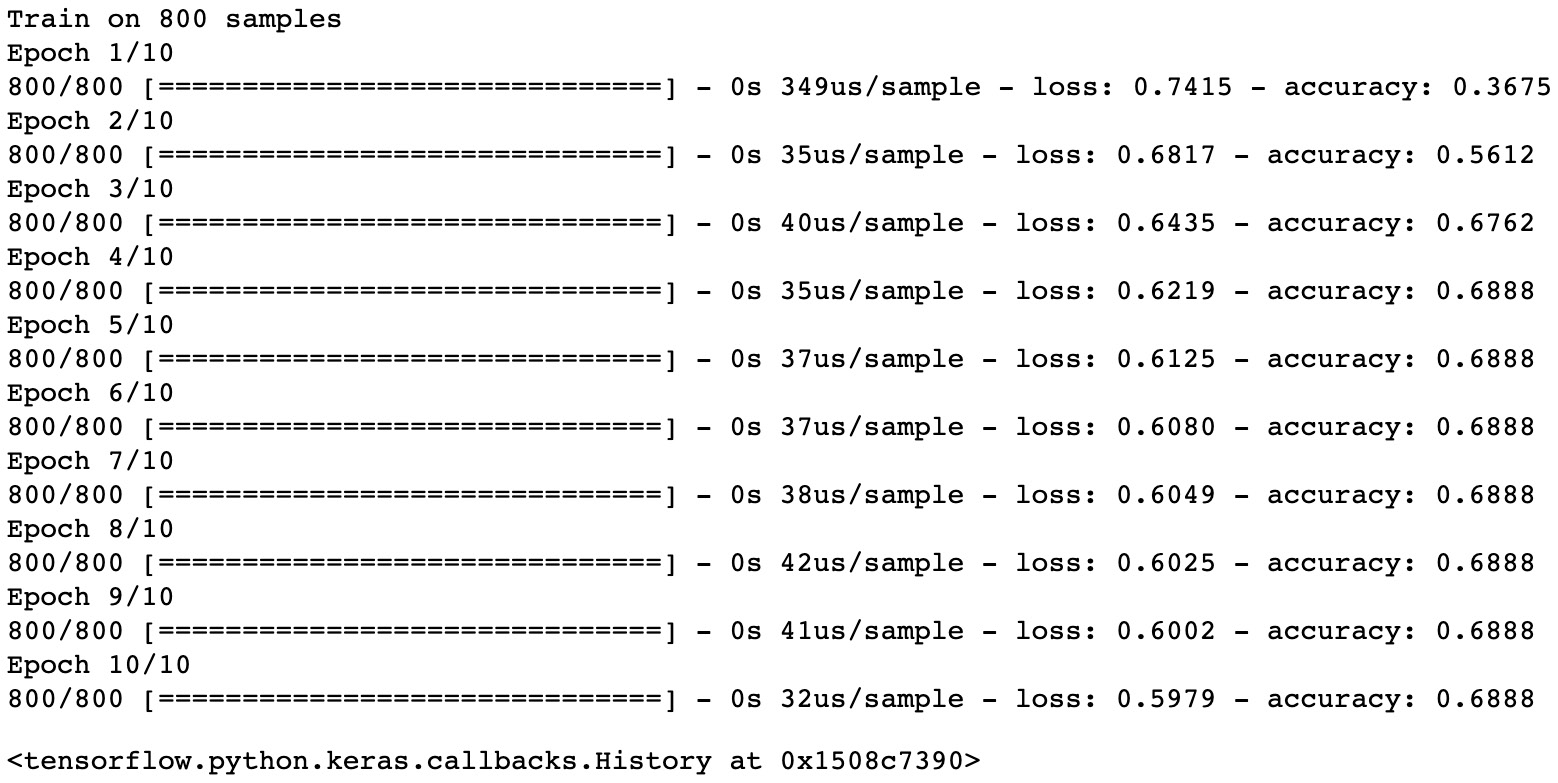
Figure 6.14: Fitting the neural network with the training set

The output provides a lot of information about the training of the neural network. The first line tells us the training set was composed of 800 observations. Then we can see the results of each epoch:

Total processing time in seconds

Processing time by data sample in us/sample

Loss value and accuracy score

The final result of this neural network is the last epoch (epoch=10), where we achieved an accuracy score of 0.6888. But we can see that the trend was improving: the accuracy score was still increasing after each epoch. So, we may get better results if we train the neural network for longer by increasing the number of epochs or lowering the learning rate.

Note

To access the source code for this specific section, please refer to https://packt.live/3fMhyLk.

You can also run this example online at https://packt.live/2Njghza. You must execute the entire Notebook in order to get the desired result.

By completing this exercise, you just trained your first classifier. In traditional machine learning algorithms, you would need to use more lines of code to achieve this, as you would have to define the entire architecture of the neural network. Here the neural network got 0.6888 after 10 epochs, but it could still improve if we let it train for longer. You can try this on your own.

Next, we will be looking at regularization.

Regularization

As with any machine learning algorithm, neural networks can face the problem of overfitting when they learn patterns that are only relevant to the training set. In such a case, the model will not be able to generalize the unseen data.

Luckily, there are multiple techniques that can help reduce the risk of overfitting:

• L1 regularization, which adds a penalty parameter (absolute value of the weights) to the loss function
• L2 regularization, which adds a penalty parameter (squared value of the weights) to the loss function
• Early stopping, which stops the training if the error for the validation set increases while the error decreases for the training set
• Dropout, which will randomly remove some neurons during training

All these techniques can be added at each layer of a neural network we create. We will be looking at this in the next exercise.

Exercise 6.04: Predicting Boston House Prices with Regularization

In this exercise, you will build a neural network that will predict the median house price for a suburb in Boston and see how to add regularizers to a network.

Note

The dataset file can also be found in our GitHub repository: https://packt.live/2V9kRUU.

Citation: The data was originally published by Harrison, D. and Rubinfeld, D.L. 'Hedonic prices and the demand for clean air', J. Environ. Economics & Management, vol.5, 81-102, 1978.

The dataset is composed of 12 different features that provide information about the suburb and a target variable (MEDV). The target variable is numeric and represents the median value of owner-occupied homes in units of $1,000.

The following steps will help you complete the exercise:

1. Open a new Jupyter Notebook file.
2. Import the pandas package as pd:

   import pandas as pd

3. Create a file_url variable containing a link to the raw dataset:

   file_url = 'https://raw.githubusercontent.com/'

              'PacktWorkshops/'

              'The-Applied-Artificial-Intelligence-Workshop'

              '/master/Datasets/boston_house_price.csv'

4. Load the dataset into a variable called df using pd.read_csv():

   df = pd.read_csv(file_url)

5. Display the first five rows using .head():

   df.head()

   The expected output is this:

   

   Figure 6.15: Output showing the first five rows of the dataset

6. Extract the target variable using .pop() and save it into a variable called label:

   label = df.pop('MEDV')

7. Import the scale function from sklearn.preprocessing:

   from sklearn.preprocessing import scale

8. Scale the DataFrame, df, and save the results into a variable called scaled_features. Print its content:

   scaled_features = scale(df)

   scaled_features

   The expected output is this:

   array([[-0.41978194, 0.28482986, -1.2879095 , ..., -0.66660821,

           -1.45900038, -1.0755623 ],

          [-0.41733926, -0.48772236, -0.59338101, ..., -0.98732948,

           -0.30309415, -0.49243937],

          [-0.41734159, -0.48772236, -0.59338101, ..., -0.98732948,

           -0.30309415, -1.2087274 ],

          ...,

          [-0.41344658, -0.48772236, 0.11573841, ..., -0.80321172,

            1.17646583, -0.98304761],

          [-0.40776407, -0.48772236, 0.11573841, ..., -0.80321172,

            1.17646583, -0.86530163],

          [-0.41500016, -0.48772236, 0.11573841, ..., -0.80321172,

   In the output, you can see that all our features are now standardized.

9. Import train_test_split from sklearn.model_selection:

   from sklearn.model_selection import train_test_split

10. Split the data into training and testing sets and save the results into four variables called features_train, features_test, label_train, and label_test. Use 10% of the data for testing and specify random_state=8:

    features_train, features_test,

    label_train, label_test = train_test_split(scaled_features,

                                               label,

                                               test_size=0.1,

                                               random_state=8)

11. Import numpy as np, tensorflow as tf, and layers from tensorflow.keras:

    import numpy as np

    import tensorflow as tf

    from tensorflow.keras import layers

12. Set 8 as the seed for NumPy and TensorFlow using np.random_seed() and tf.random.set_seed():

    np.random.seed(8)

    tf.random.set_seed(8)

13. Instantantiate a tf.keras.Sequential() class and save it into a variable called model:

    model = tf.keras.Sequential()

14. Next, create a combined l1 and l2 regularizer using tf.keras.regularizers.l1_l2 with l1=0.01 and l2=0.01. Save it into a variable called regularizer:

    regularizer = tf.keras.regularizers.l1_l2(l1=0.1, l2=0.01)

15. Instantantiate a layers.Dense() class with 10 neurons, activation='relu', input_shape=[12], and kernel_regularizer=regularizer, and save it into a variable called layer1:

    layer1 = layers.Dense(10, activation='relu',

             input_shape=[12], kernel_regularizer=regularizer)

16. Instantantiate a second layers.Dense() class with 1 neuron and save it into a variable called final_layer:

    final_layer = layers.Dense(1)

17. Add the two layers you just defined to the model using .add() and add a layer in between each of them with layers.Dropout(0.25):

    model.add(layer1)

    model.add(layers.Dropout(0.25))

    model.add(final_layer)

    We added a dropout layer in between each dense layer that will randomly remove 25% of the neurons.

18. Instantantiate a tf.keras.optimizers.SGD() class with 0.001 as the learning rate and save it into a variable called optimizer:

    optimizer = tf.keras.optimizers.SGD(0.001)

19. Compile the neural network using .compile() with loss='mse', optimizer=optimizer, metrics=['mse']:

    model.compile(loss='mse', optimizer=optimizer,

                  metrics=['mse'])

20. Print a summary of the model using .summary():

    model.summary()

    The expected output is this:

    

    Figure 6.16: Summary of the model

    This output summarizes the architecture of our neural networks. We can see it is composed of three layers with two dense layers and one dropout layer.

21. Instantiate a tf.keras.callbacks.EarlyStopping() class with monitor='val_loss' and patience=2 as the learning rate and save it into a variable called callback:

    callback = tf.keras.callbacks.EarlyStopping(monitor='val_loss',

                                                patience=2)

    We just defined a callback stating the neural network will stop its training if the validation loss (monitor='val_loss') does not improve after 2 epochs (patience=2).

22. Fit the neural networks with the training set and specify epochs=50, validation_split=0.2, callbacks=[callback], and verbose=2:

    model.fit(features_train, label_train,

              epochs=50, validation_split = 0.2,

              callbacks=[callback], verbose=2)

    The expected output is this:

    

Figure 6.17: Fitting the neural network with the training set

In the output, we see that the neural network stopped its training after the 22nd epoch. It stopped well before the maximum number of epochs, 50. This is due to the callback we set earlier: if the validation loss does not improve after two epochs, the training should stop.

Note

To access the source code for this specific section, please refer to https://packt.live/2Yobbba.

You can also run this example online at https://packt.live/37SVSu6. You must execute the entire Notebook in order to get the desired result.

You just applied multiple regularization techniques and trained a neural network to predict the median value of housing in Boston suburbs.

Activity 6.01: Finding the Best Accuracy Score for the Digits Dataset

In this activity, you will be training and evaluating a neural network that will be recognizing handwritten digits from the images provided by the MNIST dataset. You will be focusing on achieving an optimal accuracy score.

Note

You can read more about this dataset on TensorFlow's website at https://www.tensorflow.org/datasets/catalog/mnist.

Citation: This dataset was originally shared by Yann Lecun.

The following steps will help you complete the activity:

1. Import the MNIST dataset.
2. Standardize the data by applying a division by 255.
3. Create a neural network architecture with the following layers:

   A flatten input layer using layers.Flatten(input_shape=(28,28))

   A fully connected layer with layers.Dense(128, activation='relu')

   A dropout layer with layers.Dropout(0.25)

   A fully connected layer with layers.Dense(10, activation='softmax')

4. Specify an Adam optimizer with a learning rate of 0.001.
5. Define an early stopping on the validation loss and patience of 5.
6. Train the model.
7. Evaluate the model and find the accuracy score.

The expected output is this:

Figure 6.18: Expected accuracy score

Note

The solution for this activity can be found on page 378

In the next part, we will dive into deep learning topics.

Deep Learning

Now that we are comfortable in building and training a neural network with one hidden layer, we can look at more complex architecture with deep learning.

Deep learning is just an extension of traditional neural networks but with deeper and more complex architecture. Deep learning can model very complex patterns, be applied in tasks such as detecting objects in images and translating text into a different language.

Shallow versus Deep Networks

Now that we are comfortable in building and training a neural network with one hidden layer, we can look at more complex architecture with deep learning.

As mentioned earlier, we can add more hidden layers to a neural network. This will increase the number of parameters to be learned but can potentially help to model more complex patterns. This is what deep learning is about: increasing the depth of a neural network to tackle more complex problems.

For instance, we can add a second layer to the neural network we presented earlier in the section on forward propagation and loss functions:

Figure 6.19: Figure showing two hidden layers in a neural network

In theory, we can add an infinite number of hidden layers. But there is a drawback with deeper networks. Increasing the depth will also increase the number of parameters to be optimized. So, the neural network will have to train for longer. So, as good practice, it is better to start with a simpler architecture and then steadily increase its depth.

Computer Vision and Image Classification

Deep learning has achieved amazing results in computer vision and natural language processing. Computer vision is a field that involves analyzing digital images. A digital image is a matrix composed of pixels. Each pixel has a value between 0 and 255 and this value represents the intensity of the pixel. An image can be black and white and have only one channel. But it can also have colors, and in that case, it will have three channels for the colors red, green, and blue. This digital version of an image that can be fed to a deep learning model.

There are multiple applications of computer vision, such as image classification (recognizing the main object in an image), object detection (localizing different objects in an image), and image segmentation (finding the edges of objects in an image). In this book, we will only look at image classification.

In the next section, we will look at a specific type of architecture: CNNs.

Convolutional Neural Networks (CNNs)

CNNs are ANNs that are optimized for image-related pattern recognition. CNNs are based on convolutional layers instead of fully connected layers.

A convolutional layer is used to detect patterns in an image with a filter. A filter is just a matrix that is applied to a portion of an input image through a convolutional operation and the output will be another image (also called a feature map) with the highlighted patterns found by the filter. For instance, a simple filter can be one that recognizes vertical lines on a flower, such as for the following image:

Figure 6.20: Convolution detecting patterns in an image

These filters are not set in advance but learned by CNNs automatically. After the training is over, a CNN can recognize different shapes in an image. These shapes can be anywhere on the image, and the convolutional operator recognizes similar image information regardless of its exact position and orientation.

Convolutional Operations

A convolution is a specific type of matrix operation. For an input image, a filter of size n*n will go through a specific area of an image and apply an element-wise product and a sum and return the calculated value:

Figure 6.21: Convolutional operations

In the preceding example, we applied a filter to the top-left part of the image. Then we applied an element-wise product that just multiplied an element from the input image to the corresponding value on the filter. In the example, we calculated the following:

• 1st row, 1st column: 5 * 2 = 10
• 1st row, 2nd column: 10 * 0 = 0
• 1st row, 3rd column: 15 * (-1) = -15
• 2nd row, 1st column: 10 * 2 = 20
• 2nd row, 2nd column: 20 * 0 = 0
• 2nd row, 3rd column: 30 * (-1) = -30
• 3rd row, 1st column: 100 * 2 = 200
• 3rd row, 2nd column: 150 * 0 = 0
• 3rd row, 3rd column: 200 * (-1) = -200

Finally, we perform the sum of these values: 10 + 0 -15 + 20 + 0 - 30 + 200 + 0 - 200 = -15.

Then we will perform the same operation by sliding the filter to the right by one column from the input image. We keep sliding the filter until we have covered the entire image:

Figure 6.22: Convolutional operations on different rows and columns

Rather than sliding column by column, we can also slide by two, three, or more columns. The parameter defining the length of this sliding operation is called the stride.

You may have noticed that the result of the convolutional operation is an image (or feature map) with smaller dimensions than the input image. If you want to keep the exact same dimensions, you can add additional rows and columns with the value 0 around the border of the input image. This operation is called padding.

This is what is behind a convolutional operation. A convolutional layer is just the application of this operation with multiple filters.

We can declare a convolutional layer in TensorFlow with the following code snippet:

from tensorflow.keras import layers

layers.Conv2D(32, kernel_size=(3, 3), strides=(1,1),

              padding="valid", activation="relu")

In the preceding example, we have instantiated a convolutional layer with 32 filters (also called kernels) of size (3, 3) with stride of 1 (sliding window by 1 column or row at a time) and no padding (padding="valid").

Note

You can read more about this Conv2D class on TensorFlow's website, at https://www.tensorflow.org/api_docs/python/tf/keras/layers/Conv2D.

In TensorFlow, convolutional layers expect the input to be tensors with the following format: (rows, height, width, channel). Depending on the dataset, you may have to reshape the images to conform to this requirement. TensorFlow provides a function for this, shown in the following code snippet:

features_train.reshape(60000, 28, 28, 1)

Pooling Layer

Another frequent layer in a CNN's architecture is the pooling layer. We have seen previously that the convolutional layer reduces the size of the image if no padding is added. Is this behavior expected? Why don't we keep the exact same size as for the input image? In general, with CNNs, we tend to reduce the size of the feature maps as we progress through different layers. The main reason for this is that we want to have more and more specific pattern detectors closer to the end of the network.

Closer to the beginning of the network, a CNN will tend to have more generic filters, such as vertical or horizontal line detectors, but as it goes deeper, we would, for example, have filters that can detect a dog's tail or a cat's whiskers if we were training a CNN to recognize cats versus dogs, or the texture of objects if we were classifying images of fruits. Also, having smaller feature maps reduces the risk of false patterns being detected.

By increasing the stride, we can further reduce the size of the output feature map. But there is another way to do this: adding a pooling layer after a convolutional layer. A pooling layer is a matrix of a given size and will apply an aggregation function to each area of the feature map. The most frequent aggregation method is finding the maximum value of a group of pixels:

Figure 6.23: Workings of the pooling layer

In the preceding example, we use a max pooling of size (2, 2) and stride=2. We look at the top-left corner of the feature map and find the maximum value among the pixels 6, 8, 1, and 2 and get the result, 8. Then we slide the max pooling by a stride of 2 and perform the same operation on the pixels 6, 1, 7, and 4. We repeat the same operation on the bottom groups and get a new feature map of size (2,2).

In TensorFlow, we can use the MaxPool2D() class to declare a max-pooling layer:

from tensorflow.keras import layers

layers.MaxPool2D(pool_size=(2, 2), strides=2)

Note

You can read more about this Conv2D class on TensorFlow's website at https://www.tensorflow.org/api_docs/python/tf/keras/layers/MaxPool2D.

CNN Architecture

As you saw earlier, you can define your own custom CNN architecture by specifying the type and number of hidden layers, the activation functions to be used, and so on. But this may be a bit daunting for beginners. How do we know how many filters need to be added at each layer or what the right stride will be? We will have to try multiple combinations and see which ones work.

Luckily, a lot of researchers in deep learning have already done such exploratory work and have published the architecture they designed. Currently, the most famous ones are these:

• AlexNet
• VGG
• ResNet
• Inception

  Note

  We will not go through the details of each architecture as it is not in the scope of this book, but you can read more about the different CNN architectures implemented on TensorFlow at https://www.tensorflow.org/api_docs/python/tf/keras/applications.

Activity 6.02: Evaluating a Fashion Image Recognition Model Using CNNs

In this activity, we will be training a CNN to recognize clothing images that belong to 10 different classes from the Fashion MNIST dataset. We will be finding the accuracy of this CNN model.

Note

You can read more about this dataset on TensorFlow's website at https://www.tensorflow.org/datasets/catalog/fashion_mnist.

The original dataset was shared by Han Xiao.

The following steps will help you complete the activity:

1. Import the Fashion MNIST dataset.
2. Reshape the training and testing set.
3. Standardize the data by applying a division by 255.
4. Create a neural network architecture with the following layers:

   Three convolutional layers with Conv2D(64, (3,3), activation='relu') followed by MaxPooling2D(2,2)

   A flatten layer

   A fully connected layer with Dense(128, activation=relu)

   A fully connected layer with Dense(10, activation='softmax')

5. Specify an Adam optimizer with a learning rate of 0.001.
6. Train the model.
7. Evaluate the model on the testing set.

The expected output is this:

10000/10000 [==============================] - 1s 108us/sample - loss: 0.2746 - accuracy: 0.8976

[0.27461639745235444, 0.8976]

Note

The solution for this activity can be found on page 382.

In the following section, we will learn about a different type of deep learning architecture: the RNN.

Recurrent Neural Networks (RNNs)

In the last section, we learned how we can use CNNs for computer vision tasks such as classifying images. With deep learning, computers are now capable of achieving and sometimes surpassing human performance. Another field that is attracting a lot of interest from researchers is natural language processing. This is a field where RNNs excel.

In the last few years, we have seen a lot of different applications of RNN technology, such as speech recognition, chatbots, and text translation applications. But RNNs are also quite performant in predicting time series patterns, something that's used for forecasting stock markets.

RNN Layers

The common point with all the applications mentioned earlier is that the inputs are sequential. There is a time component with the input. For instance, a sentence is a sequence of words, and the order of words matters; stock market data consists of a sequence of dates with corresponding stock prices.

To accommodate such input, we need neural networks to be able to handle sequences of inputs and be able to maintain an understanding of the relationships between them. One way to do this is to create memory where the network can take into account previous inputs. This is exactly how a basic RNN works:

Figure 6.24: Overview of a single RNN

In the preceding figure, we can see a neural network that takes an input called Xt and performs some transformations and gives the output results, . Nothing new so far.

But you may have noticed that there is an additional output called Ht-1 that is an output but also an input to the neural network. This is how RNN simulates memory – by considering its previous results and taking them in as an additional input. Therefore, the result will depend on the input xt but also Ht-1. Now, we can represent a sequence of four inputs that get fed into the same neural network:

Figure 6.25: Overview of an RNN

We can see the neural network is taking an input (x) and generating an output (y) at each time step (t, t+1, …, t+3) but also another output (h), which is feeding the next iteration.

Note

The preceding figure may be a bit misleading – there is actually only one RNN here (all the RNN boxes in the middle form one neural network), but it is easier to see how the sequencing works in this format.

An RNN cell looks like this on the inside:

Figure 6.26: Internal workings of an RNN using tanh

It is very similar to a simple neuron, but it takes more inputs and uses tanh as the activation function.

Note

You can use any activation function in an RNN cell. The default value in TensorFlow is tanh.

This is the basic logic of RNNs. In TensorFlow, we can instantiate an RNN layer with layers.SimpleRNN:

from tensorflow.keras import layers

layers.SimpleRNN(4, activation='tanh')

In the code snippet, we created an RNN layer with 4 outputs and the tanh activation function (which is the most widely used activation function for RNNs).

The GRU Layer

One drawback with the previous type of layer is that the final output takes into consideration all the previous outputs. If you have a sequence of 1,000 input units, the final output, y, is influenced by every single previous result. If this sequence was composed of 1,000 words and we were trying to predict the next word, it would really be overkill to have to memorize all of the 1,000 words before making a prediction. Probably, you only need to look at the previous 100 words from the final output.

This is exactly what Gated Recurrent Unit (GRU) cells are for. Let's look at what is inside them:

Figure 6.27: Internal workings of an RNN using tanh and sigmoid

Compared to a simple RNN cell, a GRU cell has a few more elements:

• A second activation function, which is sigmoid
• A multiplier operation performed before generating the outputs and Ht

The usual path with tanh is still responsible for making a prediction, but this time we will call it the "candidate." The sigmoid path acts as an "update" gate. This will tell the GRU cell whether it needs to discard the use of this candidate or not. Remember that the output ranges between 0 and 1. If close to 0, the update gate (that is, the sigmoid path) will say we should not consider this candidate.

On the other hand, if it is closer to 1, we should definitely use the result of this candidate.

Remember that the output Ht is related to Ht-1, which is related to Ht-2, and so on. So, this update gate will also define how much "memory" we should keep. It tends to prioritize previous outputs closer to the current one.

This is the basic logic of GRU (note that the GRU cell has one more component, the reset gate, but for the purpose of simplicity, we will not look at it). In TensorFlow, we can instantiate such a layer with layers.GRU:

from tensorflow.keras import layers

layers.GRU(4, activation='tanh',

           recurrent_activation='sigmoid')

In the code snippet, we have created a GRU layer with 4 output units and the tanh activation function for the candidate prediction and sigmoid for the update gate.

The LSTM Layer

There is another very popular type of cell for RNN architecture called the LSTM cell. LSTM stands for Long Short-Term Memory. LSTM came before GRU, but the latter is much simpler, and this is the reason why we presented it first. Here is what is under the hood of LSTM:

Figure 6.28: Overview of LSTM

At first, this looks very complicated. It is composed of several elements:

• Cell state: This is the concatenation of all the previous outputs. It is the "memory" of the LSTM cell.
• Forget gate: This is responsible for defining whether we should keep or forget a given memory.
• Input gate: This is responsible for defining whether the new memory candidate needs to be updated or not. This new memory candidate is then added to the previous memory.
• Output gate: This is responsible for making the prediction based on the previous output (Ht-1), the current input (xt), and the memory.

An LSTM cell can consider previous results but also past memory, and this is the reason why it is so powerful.

In TensorFlow, we can instantiate such a layer with layers.SimpleRNN:

from tensorflow.keras import layers

layers.LSTM(4, activation='tanh',

            recurrent_activation='sigmoid')

In the code snippet, we have created an LSTM layer with 4 output units and the tanh activation function for the candidate prediction and sigmoid for the update gate.

Note

You can read more about SimpleRNN implementation in TensorFlow here: https://www.tensorflow.org/api_docs/python/tf/keras/layers/SimpleRNN.

Activity 6.03: Evaluating a Yahoo Stock Model with an RNN

In this activity, we will be training an RNN model with LSTM to predict the stock price of Yahoo! based on the data of the past 30 days. We will be finding the optimal mean squared error value and checking whether the model overfits. We will be using the same Yahoo Stock dataset that we saw in Chapter 2, An Introduction to Regression.

Note

The dataset file can also be found in our GitHub repository: https://packt.live/3fRI5Hk.

The following steps will help you to complete this activity:

1. Import the Yahoo Stock dataset.
2. Extract the close price column.
3. Standardize the dataset.
4. Create the previous 30 days' stock price features.
5. Reshape the training and testing sets.
6. Create the neural network architecture with the following layers:

   Five LSTM layers with LSTM(50, (3,3), activation='relu') followed by Dropout(0.2)

   A fully connected layer with Dense(1)

7. Specify an Adam optimizer with a learning rate of 0.001.
8. Train the model.
9. Evaluate the model on the testing set.

The expected output is this:

1000/1000 [==============================] - 0s 279us/sample - loss: 0.0016 - mse: 0.0016

[0.00158528157370165, 0.0015852816]

Note

The solution for this activity can be found on page 387.

In the next section, we will be looking at the hardware needed for deep learning.

Hardware for Deep Learning

As you may have noticed, training deep learning models takes longer than traditional machine learning algorithms. This is due to the number of calculations required for the forward pass and backpropagation. In this book, we trained very simple models with just a few layers. But there are architectures with hundreds of layers, and some with even more than that. That kind of network can take days or even weeks to train.

To speed up the training process, it is recommended to use a specific piece of hardware called a GPU. GPUs specialize in performing mathematical operations and therefore are perfect for deep learning. Compared to a Central Processing Unit (CPU), a GPU can be up to 10X faster at training a deep learning model. You can personally buy a GPU and set up your own deep learning computer. You just need to get one that is CUDA-compliant (currently only NVIDIA GPUs are).

Another possibility is to use cloud providers such as AWS or Google Cloud Platform and train your models in the cloud. You will pay only for what you use and can switch them off as soon as you are done. The benefit is that you can scale the configuration up or down depending on the needs of your projects – but be mindful of the cost. You will be charged for the time your instance is up even if you are not training a model. So, don't forget to switch things off if you're not using them.

Finally, Google recently released some new hardware dedicated to deep learning: Tensor Processing Unit (TPUs). They are much faster than GPUs, but they are quite costly. Currently, only Google Cloud Platform provides such hardware in their cloud instances.

Challenges and Future Trends

As with any new technology, deep learning comes with challenges. One of them is the big barrier to entry. To become a deep learning practitioner, you used to have to know all the mathematical theory behind deep learning very well and be a confirmed programmer. On top of this, you had to learn the specifics of the deep learning framework you chose to use (be it TensorFlow, PyTorch, Caffe, or anything else). For a while, deep learning couldn't reach a broad audience and was mainly limited to researchers. This situation has changed, though it is not perfect. For instance, TensorFlow now comes with a higher-level API called Keras (this is the one you saw in this chapter) that is much easier to use than the core API. Hopefully, this trend will keep going and make deep learning frameworks more accessible to anyone interested in this field.

The second challenge was that deep learning models require a lot of computation power, as mentioned in the previous section. This was again a major blocker for anyone who wanted to have a go at it. Even though the cost of GPUs has gone down, deep learning still requires some upfront investment. Luckily for us, there is now a free option to train deep learning models with GPUs: Google Colab. It is an initiative from Google to promote research by providing temporary cloud computing for free. The only thing you need is a Google account. Once signed up, you can create Notebooks (similar to Jupyter Notebooks) and choose a kernel to be run on a CPU, GPU (limited to 10 hours per day), or even a TPU (limited to ½ hour per day). So, before investing in purchasing or renting out GPU, you can first practice with Google Colab.

Note

You can find more information about Google Colab at https://colab.research.google.com/.

More advanced deep learning models can be very deep and require weeks of training. So, it is hard for basic practitioners to use such architecture. But thankfully, a lot of researchers have embraced the open source movement and have shared not only the architectures they have designed but also the weights of the networks. This means you can now access state-of-the-art pre-trained models and fine-tune them to fit your own projects. This is called transfer learning (which is out of the scope of this book). It is very popular in computer vision, where you can find pre-trained models on ImageNet or MS-Coco, for instance, which are large datasets of pictures. Transfer learning is also happening in natural language processing, but it is not as developed as it is for computer vision.

Note

You can find more information about these datasets at http://www.image-net.org/ and http://cocodataset.org/.

Another very important topic related to deep learning is the increasing need to be able to interpret model results. Soon, these kinds of algorithms may be regulated, and deep learning practitioners will have to be able to explain why a model is making a given decision. Currently, deep learning models are more like black boxes due to the complexity of the networks. There are already some initiatives from researchers to find ways to interpret and understand deep neural networks, such as Zeiler and Fergus, "Visualizing and Understanding Convolutional Networks", ECCV 2014. However, more work needs to be done in this field with the democratization of such technologies in our day-to-day lives. For instance, we will need to make sure that these algorithms are not biased and are not making unfair decisions affecting specific groups of people.

Summary

We have just completed the entire book of The Applied Artificial Intelligence Workshop, Second Edition. In this workshop, we have learned about the fundamentals of AI and its applications. We wrote a Python program to play tic-tac-toe. We learned about search techniques such as breadth-first search and depth-first search and how they can help us solve the tic-tac-toe game.

In the next couple of chapters after that, we learned about supervised learning using regression and classification. These chapters included data preprocessing, train-test splitting, and models that were used in several real-life scenarios. Linear regression, polynomial regression, and support vector machines all came in handy when it came to predicting stock data. Classification was performed using k-nearest neighbor and support vector classifiers. Several activities helped you to apply the basics of classification in an interesting real-life use case: credit scoring.

In Chapter 4, An Introduction to Decision Trees, you were introduced to decision trees, random forests, and extremely randomized trees. This chapter introduced different means of evaluating the utility of models. We learned how to calculate the accuracy, precision, recall, and F1 score of models. We also learned how to create the confusion matrix of a model. The models of this chapter were put into practice through the evaluation of car data.

Unsupervised learning was introduced in Chapter 5, Artificial Intelligence: Clustering, along with the k-means and hierarchical clustering algorithms. One interesting aspect of these algorithms is that the labels are not given in advance, but they are detected during the clustering process.

This workshop concluded with Chapter 6, Neural Networks and Deep Learning, where neural networks and deep learning using TensorFlow was presented. We used these techniques to achieve the best accuracy in real-life applications, such as the detection of written digits, image classification, and time series forecasting.