
CHAPTER 3
RANDOM ERROR THEORY
3.1 INTRODUCTION
As noted earlier, the adjustment of measured quantities containing random errors is a major concern to people involved in the geospatial sciences. In the remaining chapters, it is assumed that all systematic errors have been removed from the observed values and that only random error and blunders, which have escaped detection, remain. In this chapter the general theory of random errors is developed, and some simple methods that can be used to isolate blunders in sets of data are discussed.
3.2 THEORY OF PROBABILITY
![]() Probability is the ratio of the number of times that an event should occur to the total number of possibilities. For example, the probability of tossing a two with a fair die is 1/6 since there are six total possibilities (faces on a die) and only one of these is a two. When an event can occur in m ways and fail to occur in n ways, then the probability of its occurrence is m/(m + n) and the probability of its failure is n/(m + n).
Probability is the ratio of the number of times that an event should occur to the total number of possibilities. For example, the probability of tossing a two with a fair die is 1/6 since there are six total possibilities (faces on a die) and only one of these is a two. When an event can occur in m ways and fail to occur in n ways, then the probability of its occurrence is m/(m + n) and the probability of its failure is n/(m + n).
Probability is always a fraction ranging between zero and 1. Zero denotes impossibility and one indicates certainty. Since an event must either occur or fail to occur, the sum of all probabilities for any event is 1, and thus if 1/6 is the probability of throwing a two with one throw of a die, then 1 – 1/6, or 5/6 is the probability that a two will not appear.
In probability terminology, a compound event is the simultaneous occurrence of two or more independent events. This is the situation encountered most frequently in surveying. For example, random errors from angles and distances (compound events) cause traverse misclosures. The probability of the simultaneous occurrence of two independent events is the product of their individual probabilities.
To illustrate this condition, consider the simple example of having two boxes containing combinations of red and white balls. Box A contains four balls, one red and three white. Box B contains five balls, two red and three white. What is the probability that two red balls would be drawn if one ball is drawn randomly from each box? The total number of possible pairs is 4 × 5, or 20, since by drawing one ball from box A, any of the five balls in box B would complete the pair. Now, there are only two ways to draw two red balls. That is, box A's red ball can be matched with either red ball from box B. Therefore, the probability of obtaining two red balls simultaneously is 2/20. The probability of this compound event can be computed as the product of the individual probabilities of drawing a red ball from each box or
Similarly the probability of simultaneously drawing two white balls is 3/4 × 3/5 or 9/20, and the probability of getting one red and one white is 1 − (2/20 + 9/20) or 9/20.
From the foregoing, it is seen that the probability of the simultaneous occurrence of two independent events is the product of the individual probabilities of those two events. This principle is extended to include any number of events
where P is the probability of the simultaneous occurrence of events having individual probabilities P1, P2,…, Pn.
TABLE 3.1 Occurrence of Random Errors
| (1) Number of Combining Measurements |
(2) Value of Resulting Error |
(3) Frequency, t |
(4) Total Numberof Possibilities, T |
(5) Probability |
| +1 | 1 | 1/2 | ||
| 1 | −1 | 1 | 2 | 1/2 |
| +2 | 1 | 1/4 | ||
| 2 | 0 | 2 | 4 | 1/2 |
| −2 | 1 | 1/4 | ||
| +3 | 1 | 1/8 | ||
| +1 | 3 | 3/8 | ||
| 3 | −1 | 3 | 8 | 3/8 |
| −3 | 1 | 1/8 | ||
| +4 | 1 | 1/16 | ||
| +2 | 4 | 1/4 | ||
| 4 | 0 | 6 | 16 | 3/8 |
| −2 | 4 | 1/4 | ||
| −4 | 1 | 1/16 | ||
| +5 | 1 | 1/32 | ||
| +3 | 5 | 5/32 | ||
| +1 | 10 | 5/16 | ||
| 5 | −1 | 10 | 32 | 5/16 |
| −3 | 5 | 5/32 | ||
| −5 | 1 | 1/32 |
To develop the principle of how random errors occur, consider a very simple example where a single tape measurement is taken between points A and B. Assume that this measurement contains a single random error of size 1. Since the error is random, there are two possibilities for the value of the resultant error, +1 or −1. Let t be the number of ways each resultant error can occur and T be the total number of possibilities, which is two. The probability of obtaining +1, which can occur only one way (i.e., t = 1), is t/T or 1/2. This is also the probability of obtaining −1. Suppose now that in measuring a distance AE, the tape must be placed end-to-end so that the result depends on the combination of two of these tape measurements. Then the possible error combinations in the result are –1 and –1, –1 and +1, +1 and –1, and +1 and +1, with T = 4. The final errors are –2, 0, and +2, and their t values are 1, 2, and 1, respectively. This produces probabilities of 1/4, 1/2, and 1/4, respectively. In general, as n, the number of single combined measurements, is increased, T increases according to the function T = 2n, and thus for three combined measurements, T = 23 = 8, and for four measurements, T = 24 = 16.
The analysis of the preceding paragraph can be continued to obtain the results shown in Table 3.1. Figure 3.1(a) through (e) are histogram plots of the results in Table 3.1 where the values of the resultant errors are plotted as the abscissas, and the probabilities are plotted as ordinates of equal-width bars.

FIGURE 3.1 Plots of probability versus size of errors.
If the number of combining measurements, n, is increased progressively to larger values, the plot of error sizes versus probabilities would approach a smooth curve of the characteristic bell-shape shown in Figure 3.2. This curve is known as the normal error distribution curve. It is also called the probability density function of a normal random variable. Notice that when n is 4, as illustrated in Figure 3.1(d), and when n = 5, as shown in Figure 3.1(e), the dashed lines are already beginning to take on this form.

FIGURE 3.2 Normal distribution curve.
It is important to notice that the total area of the vertical bars for each plot equals 1. This is true no matter the value of n, and thus, the area under the smooth normal error distribution curve is equal to 1. If an event has a probability of 1, it is certain to occur, and therefore the area under the curve represents the sum of all the probabilities of the occurrence of errors.
As derived in Section D.1, the equation for the normal distribution curve, also called the normal probability density function, is

where f(x) is the probability density function, e the base of natural logarithms, x the error, and σ is the standard error as defined in Chapter 2.
3.3 PROPERTIES OF THE NORMAL DISTRIBUTION CURVE
In Equation (3.2), f(x) is the probability of the occurrence of an error between x and x + dx, where dx is an infinitesimally small value. The error's probability is equivalent to the area under the curve between the limits of x and x + dx, which is shown crosshatched in Figure 3.3. As stated previously, the total area under the probability curve represents the total probability, which is 1. This is represented in equation form as


FIGURE 3.3 Normal density function.
Let y represent f(x) in Equation (3.2) and differentiate

Recognizing the term in parentheses of Equation (3.4) as y gives

Taking the second derivative of Equation (3.2), we obtain

Substituting Equation (3.5) into Equation (3.6) yields

Equation (3.7) can be simplified to

From calculus, the first derivative of a function gives the slope of the function when evaluated at a point. In Equation (3.5), ![]() when the values of x or y equal zero. This implies that the curve is parallel to the x axis at the center of the curve when x is zero and is asymptotic to the x axis as y approaches zero.
when the values of x or y equal zero. This implies that the curve is parallel to the x axis at the center of the curve when x is zero and is asymptotic to the x axis as y approaches zero.
Also from calculus, a function's second derivative provides the rate of change in a slope when evaluated at a point. The curve's inflection points (points where the algebraic sign of the slope changes) can be located by finding where the function's second derivative equals zero. In Equation (3.8), ![]() when
when ![]() , and thus the curve's inflection point occurs when x equals ±σ.
, and thus the curve's inflection point occurs when x equals ±σ.
Since e0 = 1, if x is set equal to zero in Equation (3.2), then

Equation (3.9) yields the curve's central ordinate, and as can be seen, it is inversely proportional to σ. According to Equation (3.9), a group of measurements having small σ must have a large central ordinate. Thus, the area under the curve will be concentrated near the central ordinate, and the errors will be correspondingly small. This indicates that the set of measurements is precise. Since σ bears this relationship to the precision, it is a numerical measure for the precision of a measurement set. In Section 2.7, we defined σ as the standard error and gave equations for computing its value.
3.4 STANDARD NORMAL DISTRIBUTION FUNCTION
![]() In Section 3.2 we defined the probability density function of a normal random variable as
In Section 3.2 we defined the probability density function of a normal random variable as ![]() . From this, we develop the normal distribution function
. From this, we develop the normal distribution function

where t is the upper bound of integration, as shown in Figure 3.4.
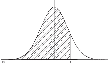
FIGURE 3.4 Area under the normal distribution curve determined by Equation (3.10).
As stated in Section 3.3, the area under the normal density curve represents the probability of occurrence. Furthermore, integration of this function yields the area under the curve. Unfortunately, the integration called for in Equation (3.10) cannot be carried out in closed form, and thus numerical integration techniques must be used to tabulate values for this function. This has been done for the function when the mean is zero (μ = 0) and the variance is 1 (σ2 = 1). The results of this integration are shown in the standard normal distribution table of Table D.1. In this table, the leftmost column with a heading of t is the value shown in Figure 3.4 in the units of σ. The top row, with headings 0 through 9, represents the hundredths decimal places for the t values. The tabulated values in the body of the Table D.1 represent areas under the standard normal distribution curve from ![]() to t. For example, to determine the area under the curve from
to t. For example, to determine the area under the curve from ![]() to 1.68, first find the row with 1.6 in the t column. Then scan along the row to the column with a heading of 8. At the intersection of row 1.6 and column 8 (1.68), the value 0.95352 occurs. This is the area under the standard normal distribution curve from
to 1.68, first find the row with 1.6 in the t column. Then scan along the row to the column with a heading of 8. At the intersection of row 1.6 and column 8 (1.68), the value 0.95352 occurs. This is the area under the standard normal distribution curve from ![]() to a t value of 1.68. Similarly, other areas under the standard normal distribution curve can be found for various values for t. Since the area under the curve represents probability, and its maximum area is 1, this means that there is a 95.352% (0.95352 × 100%) probability that t is less than or equal to 1.68. Alternatively, it can be stated that there is a 4.648% (1 − 0.95352) × 100% probability that t is greater than 1.68.
to a t value of 1.68. Similarly, other areas under the standard normal distribution curve can be found for various values for t. Since the area under the curve represents probability, and its maximum area is 1, this means that there is a 95.352% (0.95352 × 100%) probability that t is less than or equal to 1.68. Alternatively, it can be stated that there is a 4.648% (1 − 0.95352) × 100% probability that t is greater than 1.68.
Once available, Table D.1 can be used to evaluate the distribution function for any mean, μ, and variance, σ2. For example, if y is a normal random variable with a mean of μ and a variance of σ2, an equivalent normal random variable ![]() can be defined that has a mean of zero and a variance of 1. Substituting the definition for z with
can be defined that has a mean of zero and a variance of 1. Substituting the definition for z with ![]() and
and ![]() into Equation (3.2), its density function is
into Equation (3.2), its density function is

and its distribution function, which is known as the standard normal distribution function, becomes

For any group of normally distributed measurements, the probability of the normal random variable can be computed by analyzing the integration of the distribution function. Again, as stated previously, the area under the curve in Figure 3.4 represents probability. Let z be a normal random variable, then the probability that z is less than some value of t is given by
To determine the area (probability) between t values of a and b (the crosshatched areas in Figures 3.5 and 3.6), the difference in the areas between a and b, respectively, can be computed. By Equation (3.13), the area from ![]() to b is
to b is ![]() . By the same equation, the area from
. By the same equation, the area from ![]() to a is
to a is ![]() . Thus the area between a and b is the difference in these values and is expressed as
. Thus the area between a and b is the difference in these values and is expressed as

FIGURE 3.5 Area representing the probability in Equation (3.14).

FIGURE 3.6 Area representing the probability in Equation (3.16).
If the bounds are equal in magnitude but opposite in sign, that is, ![]() , the probability is
, the probability is
From the symmetry of the normal distribution in Figure 3.6, it is seen that
for any t > 0. Also, this symmetry can be seen with Table D.1. The tabular value (area) for a t value of −1.00 is 0.15866. Furthermore, the tabular value for a t value of +1.00 is 0.84134. Since the maximum probability (area) is 1, the area above +1.00 is 1 − 0.84134, or 0.15866, which is the same as the area below −1.00. Thus, since the total probability is always 1, we can define the following relationship
Now substituting Equation (3.17) into Equation (3.15), we have

FIGURE 3.7 Normal distribution curve.
3.5 PROBABILITY OF THE STANDARD ERROR
The preceding equations can be used to determine the probability of the standard error, which from previous discussion is the area under the normal distribution curve between the limits of ±σ. For the standard normal distribution when σ2 is 1, it is necessary to locate the values of ![]() and
and ![]() in Table D.1. As seen previously, the appropriate value from the table for t = −1.00 is 0.15866. Also, the tabular value for t = 1.00 is 0.84134, and thus, according to Equation (3.15), the area between −σ and +σ is
in Table D.1. As seen previously, the appropriate value from the table for t = −1.00 is 0.15866. Also, the tabular value for t = 1.00 is 0.84134, and thus, according to Equation (3.15), the area between −σ and +σ is

From this it has been determined that approximately 68.3% of all measurements from any data set are expected to lie between −σ and +σ. It also means that for any group of measurements there is approximately a 68.3% chance that any single observation has an error between ±σ. The crosshatched area of Figure 3.7 illustrates that approximately 68.3% of the area exists between ±σ. This is true for any set of measurements having normally distributed errors. Note that as discussed in Section 3.3, the inflection points of the normal distribution curve occur at ±σ. This is illustrated in Figure 3.7.
3.5.1 The 50% Probable Error
For any group of observations, the 50% probable error establishes the limits within which 50% of the errors should fall. In other words, any measurement has the same chance of coming within these limits as it has of falling outside them. Its value can be obtained by multiplying the observations' standard deviation by the appropriate t value. Since the 50% probable error has a probability of one-half, Equation (3.18) is set equal to 0.50 and the t value corresponding to this area is determined as

From Table D.1 it is apparent that 0.75 is between a t value of 0.67 and 0.68; that is,
The t value can be found by linear interpolation, as follows

and ![]() . Thus, the equation for linear interpolation can be expressed as
. Thus, the equation for linear interpolation can be expressed as

where t is the desired t value, tl and tu the lower and upper t values that bound t, Nz(t) the desired value from the table, and Nz(tl), and Nz(tu), the tabular values that bound Nz(t). Thus, the previous example could be completed in one computation as
For any set of observations, therefore, the 50% probable error can be obtained by computing the standard error and then multiplying it by 0.6745, or
3.5.2 The 95% Probable Error
The 95% probable error, or E95, is the bound within which, theoretically, 95% of the observation group's errors should fall. This error category is popular with surveyors for expressing precision and checking for outliers in data. Using the same reasoning as in developing the equation for the 50% probable error, substituting into Equation (3.18), yields

Again from the Table D.1, it is determined that 0.975 occurs with a t value of 1.960. Thus, to find the 95% probable error for any group of measurements, the following equation is used
3.5.3 Other Percent Probable Errors
Using the same computation techniques as in Sections 3.5.1 and 3.5.2, other percent probable errors can be calculated. One other percent error worthy of particular note is E99.7. It is obtained by multiplying the standard error by 2.968, or
This value is often used for detecting blunders, as discussed in Section 3.6. A summary of probable errors with varying percentages, together with their multipliers, is given in Table 3.2.
TABLE 3.2 Multipliers for Various Percent Probable Errors
| Symbol | Multiplier | Percent Probable Errors |
| E50 | 0.6745σ | 50 |
| E90 | 1.645σ | 90 |
| E95 | 1.960σ | 95 |
| E99 | 2.57σ | 99 |
| E99.7 | 2.968σ | 99.7 |
| E99.9 | 3.29σ | 99.9 |
3.6 USES FOR PERCENT ERRORS
Standard errors and errors of other percent probabilities are commonly used to evaluate measurements for acceptance. Project specifications and contracts often require that acceptable errors be within specified limits such as the 90% and 95% errors. The 95% error, sometimes called the two-sigma (2σ) error because it is computed as approximately 2σ, is most often specified. Standard error is also frequently used. The probable error, E50, is seldom employed.
Higher-percentage errors are used to help isolate outliers (very large errors) and blunders in data sets. Since outliers seldom occur in a data set, measurements outside a selected high percentage range can be rejected as possible blunders. Generally, any data that differ from the mean by more than 3σ can be considered as blunders and removed from a data set. As seen in Table 3.2, rejecting observations greater than 3σ means that about 99.7% of all observations should be retained. In other words, only about 0.3% of the observations in a set of normally distributed random errors (or 3 observations in 1000) should lie outside the range of ±3σ.
Note that as explained in Chapter 2, standard error and standard deviation are often used interchangeably, when in practice, it is actually the standard deviation that is computed, not the standard error. Thus, for practical applications, σ in the equations of the preceding sections is replaced by S to distinguish between these two related values.
3.7 PRACTICAL EXAMPLES
PROBLEMS
Note: Partial answers to problems marked with an asterisk are given in Appendix H.
- *3.1 Determine the t value for E80.
- 3.2 Determine the t value for E99.7.
- 3.3 Determine the t value for E90.
- 3.4 Determine the t value for E99.9.
- 3.5 Define probability.
- 3.6 Define compound event.
- *3.7 If the mean of a population is 2.456 and its variance is 2.042, what is the peak value for the normal distribution curve, and the x coordinates for the points of inflection?
- 3.8 If the mean of a population is 25.8 and its variance is 3.6, what is the peak value for the normal distribution curve, and the x coordinates for the points of inflection?
- 3.9 If the mean of a population is 10.3 and its variance is 1.9, what is the peak value for the normal distribution curve, and the x coordinates for the points of inflection?
- 3.10 Plot the curve in Problem 3.7 using Equation (3.2) to determine ordinate and abscissa values.
- 3.11 Plot the curve in Problem 3.8 using Equation (3.2) to determine ordinate and abscissa values.
- 3.12 Plot the curve in Problem 3.9 using Equation (3.2) to determine ordinate and abscissa values.
- 3.13 The following data represent 21 electronically measured distance observations.
485.62 485.62 485.63 485.59 485.66 485.62 485.61 485.59 485.62 485.65 485.64 485.65 485.61 485.64 485.62 485.64 485.64 485.61 485.68 485.61 485.63 - *(a) Calculate the mean and the standard deviation.
- (b) Plot the relative frequency histogram (of residuals) for the data above using a five class intervals.
- (c) Calculate the E50 and E90 intervals.
- (d) Can any observations be rejected at a 95% level of certainty?
- (e) What is the peak value for the normal distribution curve and where are the points of inflection on the curve on the x axis?
- *3.14 Using the data in Problem 2.12, calculate the E95 interval and identify any observations that can be rejected at a 95% level of certainty.
- 3.15 Repeat Problem 3.14 for the data in Problem 2.15.
- 3.16 Discuss the normality of each set of data below and whether any observations may be removed at the 99% level of certainty as blunders or outliers. Determine which set is more precise after apparent blunders and outliers are removed. Plot the relative frequency histogram to defend your decisions.
Set 1: 468.09 468.13 468.11 468.13 468.10 468.13 468.12 468.09 468.14 468.10 468.10 468.12 468.14 468.16 468.12 468.10 468.10 468.11 468.13 468.12 468.18 Set 2: 750.82 750.86 750.83 750.88 750.88 750.86 750.86 750.85 750.86 750.86 750.88 750.84 750.84 750.88 750.86 750.87 750.86 750.83 750.90 750.84 750.86 - 3.17 Using the following data set, answer the questions below.
46.5 45.2 48.4 38.2 54.7 46.0 38.5 46.2 53.4 50.9 53.7 44.1 45.1 49.8 49.7 42.9 56.7 42.5 43.6 50.5 48.5 43.3 46.2 49.1 45.4 56.4 48.2 44.9 47.8 43.1 - (a) What are the mean and standard deviation of the data set?
- (b) Construct a relative frequency histogram of the data using seven intervals and discuss whether it appears to be a normal data set.
- (c) What is the E95 interval for this data set?
- (d) Would there be any reason to question the validity of any observation at the 95% level?
- 3.18 Repeat Problem 3.17 using the following data:
122.34 122.34 122.35 122.30 122.38 122.34 122.31 122.34 122.37 122.36 122.37 122.33 122.34 122.36 122.36 122.33 122.38 122.33 122.33 122.36 - 3.19 What is the E95 interval for the following data? Is there any reason to question the validity of any observation at the 95% level?
8.6 8.5 8.9 7.4 9.6 8.6 7.7 8.6 9.4 9.1 9.5 8.3 8.4 9.0 9.0 8.2 9.8 8.1 8.3 9.1 - 3.20 Using the data from Problem 3.19, what is the E99 interval for the following data? Is there any reason to question the validity of any observation at the 99% level?
Use STATS to do Problems 3.21 and 3.22.
- 3.21 Problem 3.16.
- 3.22 Problem 3.17.
PROGRAMMING PROBLEMS
- 3.23 Create a spreadsheet to solve Problem 3.13.
- 3.24 Create a computation package to solve Problem 3.19.