
A multivariable linear regression model can have multiple variables or features, as opposed to the linear regression model with a single variable that we previously studied. Interestingly, the definition of a linear model with a single variable can itself be extended via matrices to be applied to multiple variables.
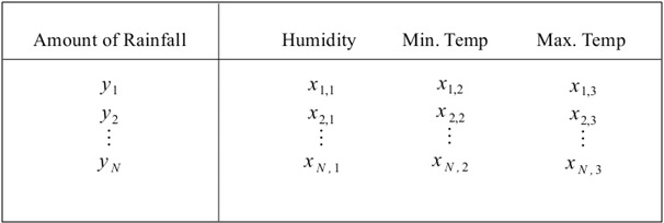
We can extend our previous example for predicting the probability of rainfall on a particular day to a model with multiple variables by including more independent variables, such as the minimum and maximum temperatures, in the sample data. Thus, the training data for a multivariable linear regression model will look similar to the following illustration:
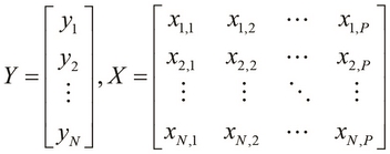
For a multivariable linear regression model, the training data is defined by two matrices, X and Y. Here, X is an ![]() matrix, where P is the number of independent variables in the model. The matrix Y is a vector of length N, just like in a linear model with a single variable. This model is illustrated as follows:
matrix, where P is the number of independent variables in the model. The matrix Y is a vector of length N, just like in a linear model with a single variable. This model is illustrated as follows:
For the following example of multivariable linear regression in Clojure, we will not generate the sample data through code but use the sample data from the Incanter library. We can fetch any dataset using the Incanter library's get-dataset function.
We can fetch the Iris dataset by calling the get-dataset function with the :iris keyword argument; this is shown as follows:
(def iris
  (to-matrix (get-dataset :iris)))

(def X (sel iris :cols (range 1 5)))
(def Y (sel iris :cols 0))
We first define the variable iris as a matrix using the to-matrix and get-dataset functions, and then define two matrices X and Y. Here, Y is actually a vector of 150 values, or a matrix of size ![]() , while
, while X is a matrix of size ![]() . Hence,
. Hence, X can be used to represent the values of four independent variables, and Y represents the values of the dependent variable. Note that the sel function is used to select a set of columns from the iris matrix. In fact, we could select many more such columns from the iris data matrix, but we will use only four in the following example for the sake of simplicity.
Note
The dataset that we used in the previous code example is the Iris dataset, which is available in the Incanter library. This dataset has quite a bit of historical significance, as it was used by Sir Ronald Fisher to first develop the linear discriminant analysis (LDA) method for classification (for more information, refer to "The Species Problem in Iris"). This dataset contains 50 samples of three distinct species of the Iris plant, namely Setosa, Versicolor, and Virginica. Four features of the flowers of these species are measured in each sample, namely the petal width, petal length, sepal width, and sepal length. Note that we will encounter this dataset several times over the course of this book.
Interestingly, the linear-model function accepts a matrix with multiple columns, so we can use this function to fit a linear regression model over both single variable and multivariable data as follows:
(def iris-linear-model
  (linear-model Y X))
(defn plot-iris-linear-model []
  (let [x (range -100 100)
        y (:fitted iris-linear-model)]
    (view (xy-plot x y :x-label "X" :y-label "Y"))))

(plot-iris-linear-model)
In the preceding code example, we plot the linear model using the xy-plot function while providing optional parameters to specify the labels of the axes in the defined plot. Also, we specify the range of the x axis by generating a vector using the range function. The plot-iris-linear-model function generates the following plot:
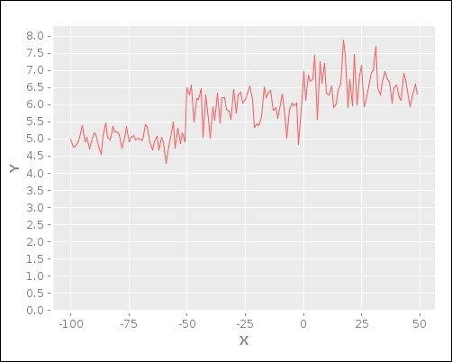
Although the curve in the plot produced from the previous example doesn't appear to have any definitive shape, we can still use this generated model to estimate or predict the value of the dependent variable by supplying values for the independent variables to the formulated model. In order to do this, we must first define the relationship between the dependent and independent variables of a linear regression model with multiple features.
A linear regression model of P independent variables produces ![]() regression coefficients, since we include the error constant along with the other coefficients of the model and also define an extra variable
regression coefficients, since we include the error constant along with the other coefficients of the model and also define an extra variable ![]() , which is always 1.
, which is always 1.
The linear-model function agrees with the proposition that the number of coefficients P in the formulated model is always one more than the total number of independent variables in the sample data N; this is shown in the following code:
user> (= (count (:coefs iris-linear-model))
         (+ 1 (column-count X)))
true
We formally express the relationship between a multivariable regression model's dependent and independent variables as follows:
Since the variable ![]() is always 1 in the preceding equation, the value
is always 1 in the preceding equation, the value ![]() is analogous to the error constant
is analogous to the error constant ![]() from the definition of a linear model with a single variable.
from the definition of a linear model with a single variable.
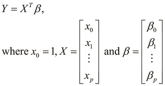
We can define a single vector to represent all the coefficients of the previous equation as ![]() . This vector is termed as the
parameter vector of the formulated regression model. Also, the independent variables of the model can be represented by a vector. Thus, we can define the regression variable Y as the product of the transpose of the parameter vector and the vector of independent variables of the model:
. This vector is termed as the
parameter vector of the formulated regression model. Also, the independent variables of the model can be represented by a vector. Thus, we can define the regression variable Y as the product of the transpose of the parameter vector and the vector of independent variables of the model:
Polynomial functions can also be reduced to the standard form by substituting a single variable for every higher-order variable in the polynomial equation. For example, consider the following polynomial equation:
We can substitute the variables ![]() for
for ![]() to reduce the equation to the standard form of a multivariable linear regression model.
to reduce the equation to the standard form of a multivariable linear regression model.
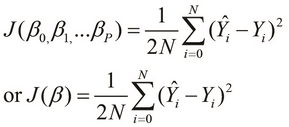
This brings us to the following formal definition of the cost function for a linear model with multiple variables, which is simply an extension of the definition of the cost function for a linear model with a single variable:
Note that in the preceding definition, we can use the individual coefficients of the model interchangeably with the parameter vector ![]() .
.
Analogous to our problem definition of fitting a model with a single variable over some given data, we can define the problem of formulating a multivariable linear model as the problem of minimizing the preceding cost function:
We can apply the gradient descent algorithm to find the local minimum of a model with multiple variables. Of course, since we have multiple coefficients in the model, we have to apply the algorithm for all these coefficients as opposed to just two coefficients in a regression model with a single variable.
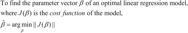
The gradient descent algorithm can thus be used to find the values of all the coefficients in the parameter vector ![]() of a multivariable linear regression model, and is formally defined as follows:
of a multivariable linear regression model, and is formally defined as follows:
In the preceding definition, the term ![]() simply refers to the sample values for the
simply refers to the sample values for the ![]() independent variable in the formulated model. Also, the variable
independent variable in the formulated model. Also, the variable ![]() is always 1. Thus, this definition can be applied to just the two coefficients that correspond to our previous definition of the gradient descent algorithm for a linear regression model with a single variable.
is always 1. Thus, this definition can be applied to just the two coefficients that correspond to our previous definition of the gradient descent algorithm for a linear regression model with a single variable.
As we've seen earlier, the gradient descent algorithm can be applied to a linear regression model with both single and multivariables. For some models, however, the gradient descent algorithm can actually take a lot of iterations, or rather time, to converge the estimated values of the model's coefficients. Sometimes, the algorithm can also diverge, and thus we will be unable to calculate the model's coefficients in such circumstances. Let's examine some of the factors that affect the behavior and performance of this algorithm:
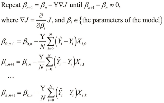
- All the features of the sample data must be scaled with respect to each other. By scaling, we mean that all the values for the independent variables in the sample data take on a similar range of values. Ideally, all independent variables must have observed values between -1 and 1. This can be formally expressed as follows:
-
We can normalize the observed values for the independent variables about the mean of these values. We can further normalize this data by using the standard deviation of the observed values. In summary, we substitute the values with those produced by subtracting the mean of these values,
 ,and dividing the resulting expression by the standard deviation
  . This is shown in the following formula:
-
The stepping or learning rate,
 , is another important factor that determines how fast the algorithm converges towards the values of the parameters of the formulated model. Ideally, the stepping rate should be selected so that the differences between the old and new iterated values of the parameters of the model have an optimal amount of change in every iteration. On one hand, if this value is too large, the algorithm could even produce diverging values for the parameters of the model after each iteration. Thus, the algorithm will never find a global minimum in this case. On the other hand, a small value for this rate could result in slowing down the algorithm through an unnecessarily large number of iterations.