
Another technique to estimate the parameter vector of a linear regression model is the Ordinary Least Squares (OLS) method. The OLS method essentially works by minimizing the sum of squared errors in a linear regression model.
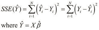
The sum of squared errors of prediction, or SSE, of a linear regression model can be defined in terms of the model's actual and expected values as follows:
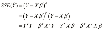
The preceding definition of the SSE can be factorized using matrix products as follows:
We can solve the preceding equation for the estimated parameter vector ![]() by using the definition of a global minimum. Since this equation is a form of quadratic equation and the term
by using the definition of a global minimum. Since this equation is a form of quadratic equation and the term ![]() is always greater than zero, the global minimum of the surface of the cost function can be defined as the point at which the rate of change of the slope of a tangent to the surface at that point is zero. Also, the plot is a function of the parameters of the linear model, and so the equation of the surface plot should be differentiated by the estimated parameter vector
is always greater than zero, the global minimum of the surface of the cost function can be defined as the point at which the rate of change of the slope of a tangent to the surface at that point is zero. Also, the plot is a function of the parameters of the linear model, and so the equation of the surface plot should be differentiated by the estimated parameter vector ![]() . We can thus solve this equation for the optimal parameter vector
. We can thus solve this equation for the optimal parameter vector ![]() of the formulated model as follows:
of the formulated model as follows:
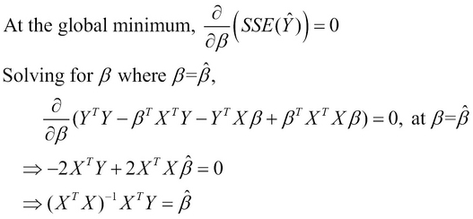
The last equation in the preceding derivation gives us the definition of the optimal parameter vector ![]() , which is formally expressed as follows:
, which is formally expressed as follows:
We can implement the preceding definition of the parameter vector through the OLS method using the core.matrix library's transpose and inverse functions and the Incanter library's bind-columns function:
(defn linear-model-ols
  "Estimates the coefficients of a multi-var linear
  regression model using Ordinary Least Squares (OLS) method"
  [MX MY]
  (let [X (bind-columns (repeat (row-count MX) 1) MX)
        Xt (cl/matrix (transpose X))
        Xt-X (cl/* Xt X)]
    (cl/* (inverse Xt-X) Xt MY)))

(def ols-linear-model
  (linear-model-ols X Y))

(def ols-linear-model-coefs
  (cl/as-vec ols-linear-model))
Here, we first add a column in which each element is 1, as the first column of the matrix MX uses the bind-columns function. The extra column that we add represents the independent variable ![]() , whose value is always
, whose value is always 1. We then use the transpose and inverse functions to calculate the estimated coefficients of the linear regression model for the data in matrices MX and MY.
The previously defined function can be applied to the matrices that we have previously defined (X and Y) as follows:
(def ols-linear-model
  (linear-model-ols X Y))

(def ols-linear-model-coefs
  (cl/as-vec ols-linear-model))
In the preceding code, ols-linear-model-coefs is simply the variable and ols-linear-model is a matrix with a single column, which is represented as a vector. We perform this conversion using the as-vec function from the clatrix library.
We can actually verify that the coefficients estimated by the ols-linear-model function are practically equal to the ones generated by the Incanter library's linear-model function, which is illustrated as follows:
user> (cl/as-vec (ols-linear-model X Y))
[1.851198344985435 0.6252788163253274 0.7429244752213087 -0.4044785456588674 -0.22635635488532463]
user> (:coefs iris-linear-model)
[1.851198344985515 0.6252788163253129 0.7429244752213329 -0.40447854565877606 -0.22635635488543926]
user> (every? #(< % 0.0001)
                      (map -
                         ols-linear-model-coefs
                         (:coefs iris-linear-model)))
true
In the last expression in the preceding code example, we find the difference between the coefficients produced by the ols-linear-model function, the difference produced by the linear-model function, and check whether each of these differences is less than 0.0001.