
We now introduce a simple model of feed-forward neural networks—the Multilayer Perceptron model. This model represents a basic feed-forward neural network and is versatile enough to model regression and classification problems in the domain of supervised learning. All the input flows through a feed-forward neural network in a single direction. This is a direct consequence of the fact that there is no feedback from or to any layer in a feed-forward neural network.
By feedback, we mean that the output of a given layer is fed back as input to the perceptrons in a previous layer in the ANN. Also, using a single layer of perceptrons would mean using only a single activation function, which is equivalent to using logistic regression to model the given training data. This would mean that the model cannot be used to fit nonlinear data, which is the primary motivation of ANNs. We must note that we discussed logistic regression in Chapter 3, Categorizing Data.
A multilayer perceptron ANN can be illustrated by the following diagram:
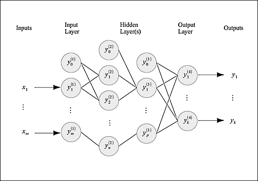
A multilayer perceptron ANN comprises several layers of perceptron nodes. It exhibits a single input layer, a single output layer, and several hidden layers of perceptrons. The input layer simply relays the input values to the first hidden layer of the ANN. These values are then propagated to the output layer through the other hidden layers, where they are weighted and summed using the activation function, to finally produce the output values.
Each sample in the training data is represented by the ![]() tuple, where
tuple, where ![]() is the expected output and
is the expected output and ![]() is the input value of the
is the input value of the ![]() training sample. The
training sample. The ![]() input vector comprises a number of values equal to the number of features in the training data.
input vector comprises a number of values equal to the number of features in the training data.
The output of each node is termed as the activation of the node and is represented by the term ![]() for the
for the ![]() node in the layer
node in the layer ![]() . As we mentioned earlier, the activation function used to produce this value is the sigmoid function or the hyperbolic tangent function. Of course, any other mathematical function could be used to fit the sample data. The input layer of a multilayer perceptron network simply adds a bias input to the input values, and the set of inputs supplied to the ANN are relayed to the next layer. We can formally represent this equality as follows:
. As we mentioned earlier, the activation function used to produce this value is the sigmoid function or the hyperbolic tangent function. Of course, any other mathematical function could be used to fit the sample data. The input layer of a multilayer perceptron network simply adds a bias input to the input values, and the set of inputs supplied to the ANN are relayed to the next layer. We can formally represent this equality as follows:
The synapses between every pair of layers in the ANN have an associated weight matrix. The number of rows in these matrices is equal to the number of input values, that is, the number of nodes in the layer closer to the input layer of the ANN and the number of columns equal to the number of nodes in the layer of the synapse that is closer to the output layer of the ANN. For a layer l, the weight matrix is represented by the term ![]() .
.
The activation values of a layer l can be determined using the activation function of the ANN. The activation function is applied on the products of the weight matrix and the activation values produced by the previous layer in the ANN. Generally, the activation function used for a multilayer perceptron is a sigmoid function. This equality can be formally represented as follows:
Generally, the activation function used for a multilayer perceptron is a sigmoid function. Note that we do not add a bias value in the output layer of an ANN. Also, the output layer can produce any number of output values. To model a k-class classification problem, we would require an ANN producing k output values.
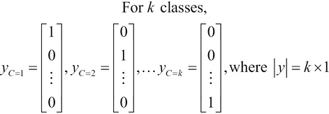
To perform binary classification, we can only model a maximum of two classes of input data. The output value generated by an ANN used for binary classification is always 0 or 1. Thus, for ![]() classes,
classes, ![]() .
.
We can also model a multiclass classification using the k binary output values, and thus, the output of the ANN is a ![]() matrix. This can be formally expressed as follows:
matrix. This can be formally expressed as follows:
Hence, we can use a multilayer perceptron ANN to perform binary and multiclass classifications. A multilayer perceptron ANN can be trained using the backpropagation algorithm, which we will study and implement later in this chapter.
Let's assume that we want to model the behavior of a logical XOR gate. An XOR gate can be thought of a binary classifier that requires two inputs and generates a single output. An ANN that models the XOR gate would have a structure as shown in the following diagram. Interestingly, linear regression can be used to model both AND and OR logic gates but cannot be used to model an XOR gate. This is due to the nonlinear nature of the output of an XOR gate, and thus, ANNs are used to overcome this limitation.
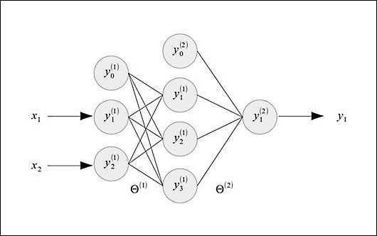
The multilayer perceptron illustrated in the preceding diagram has three nodes in the input layer, four nodes in the hidden layer, and one node in the output layer. Observe that every layer other than the output layer adds a bias input to the set of input values for the nodes in the next layer. There are two synapses in the ANN, shown in the preceding diagram, and they are associated with the weight matrices ![]() and
and ![]() . Note that the first synapse is between the input layer and hidden layer, and the second synapse is between the hidden layer and the output layer. The weight matrix
. Note that the first synapse is between the input layer and hidden layer, and the second synapse is between the hidden layer and the output layer. The weight matrix ![]() has a size of
has a size of ![]() , and the weight matrix
, and the weight matrix ![]() has a size of
has a size of ![]() . Also, the term
. Also, the term ![]() is used to represent all the weight matrices in the ANN.
is used to represent all the weight matrices in the ANN.
As the activation function of each node in a multilayer perceptron ANN is a sigmoid function, we can define the cost function of the weights of the nodes of the ANN similar to the cost function of a logistic regression model. The cost function of an ANN can be defined in terms of the weight matrices as follows:
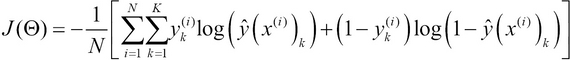
The preceding cost function is essentially the average of the cost functions of each node in the output layer of an ANN (for more information, refer to Neural Networks in Materials Science). For a multilayer perceptron ANN with K output values, we perform the average over the K terms. Note that ![]() represents the
represents the ![]() output value of the ANN,
output value of the ANN, ![]() represents the input variables of the ANN, and N is the number of sample values in the training data. The cost function is essentially that of logistic regression but is applied here for the K output values. We can add a regularization parameter to the preceding cost function and express the regularized cost function using the following equation:
represents the input variables of the ANN, and N is the number of sample values in the training data. The cost function is essentially that of logistic regression but is applied here for the K output values. We can add a regularization parameter to the preceding cost function and express the regularized cost function using the following equation:

The cost function defined in the preceding equation adds a regularization term similar to that of logistic regression. The regularization term is essentially the sum of the squares of all weights of all input values of the several layers of the ANN, excluding the weights for the added bias input. Also, the term ![]() refers to the number of nodes in layer l of the ANN. An interesting point to note is that in the preceding regularized cost function, only the regularization term depends on the number of layers in the ANN. Hence, the generalization of the estimated model is based on the number of layers in the ANN.
refers to the number of nodes in layer l of the ANN. An interesting point to note is that in the preceding regularized cost function, only the regularization term depends on the number of layers in the ANN. Hence, the generalization of the estimated model is based on the number of layers in the ANN.