
In some cases, the available training data is not linearly separable and we would not be able to model the data using linear classification. Thus, we need to use different models to fit nonlinear data. As described in Chapter 4, Building Neural Networks, ANNs can be used to model this kind of data. In this section, we will describe how we can fit an SVM on nonlinear data using kernel functions. An SVM that incorporates kernel function is termed as a kernel support vector machine. Note that, in this section, the terms SVM and kernel SVM are used interchangeably. A kernel SVM will classify data based on a nonlinear decision boundary, and the nature of the decision boundary depends on the kernel function that is used by the SVM. To illustrate this behavior, a kernel SVM will classify the training data into two classes as described by the following plot diagram:
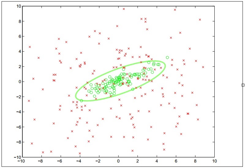
The concept of using kernel functions in SVMs is actually based on mathematical transformation. The role of the kernel function in an SVM is to transform the input variables in the training data such that the transformed features are linearly separable. Since an SVM linearly partitions the input data based on a large margin, this large gap of separation between the two classes of data will also be observable in a nonlinear space.
The kernel function is written as ![]() , where
, where ![]() is a vector of input values from the training data and
is a vector of input values from the training data and ![]() is the transformed vector of
is the transformed vector of ![]() . The function
. The function ![]() represents the similarity of these two vectors and is equivalent to the inner product of these two vectors in the transformed space. If the input vector
represents the similarity of these two vectors and is equivalent to the inner product of these two vectors in the transformed space. If the input vector ![]() has a given class, then the class of the vector
has a given class, then the class of the vector ![]() is the same as that of the vector
is the same as that of the vector ![]() when the kernel function of these two vectors has a value close to 1, that is, when
when the kernel function of these two vectors has a value close to 1, that is, when ![]() . A kernel function can be mathematically expressed as follows:
. A kernel function can be mathematically expressed as follows:
In the preceding equation, the function ![]() performs the transformation from a nonlinear space
performs the transformation from a nonlinear space ![]() into a linear space
into a linear space ![]() . Note that the explicit representation of
. Note that the explicit representation of ![]() is not required, and it's enough to know that
is not required, and it's enough to know that ![]() is an inner product space. Although we are free to choose any arbitrary kernel function to model the given training data, we must strive to reduce the problem of minimizing the cost function of the formulated SVM model. Thus, the kernel function is generally selected such that calculating the SVM's decision boundary only requires determining the dot products of vectors in the transformed feature space
is an inner product space. Although we are free to choose any arbitrary kernel function to model the given training data, we must strive to reduce the problem of minimizing the cost function of the formulated SVM model. Thus, the kernel function is generally selected such that calculating the SVM's decision boundary only requires determining the dot products of vectors in the transformed feature space ![]() .
.
A common choice for the kernel function of an SVM is the polynomial kernel function, also called the polynomic kernel function, which models the training data as polynomials of the original feature variables. As the reader may recall from Chapter 5, Selecting and Evaluating Data, we have discussed how polynomial features can greatly improve the performance of a given machine learning model. The polynomial kernel function can be thought of as an extension of this concept that applies to SVMs. This function can be formally expressed as follows.
In the preceding equation, the term ![]() represents the highest degree of the polynomial features. Also, when (the constant)
represents the highest degree of the polynomial features. Also, when (the constant) ![]() , the kernel is termed to be homogenous.
, the kernel is termed to be homogenous.
Another widely used kernel function is the Gaussian kernel function. Most readers who are adept in linear algebra will need no introduction to the Gaussian function. It's important to know that this function represents a normal distribution of data in which the data points are closer to the mean of the data.
In the context of SVMs, the Gaussian kernel function can be used to represent a model in which one of the two classes in the training data has values for the input variables that are close to an arbitrary mean value. The Gaussian kernel function can be formally expressed as follows:
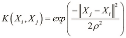
In the Gaussian kernel function defined in the preceding equation, the term ![]() represents the variance of the training data and represents the width of the Gaussian kernel.
represents the variance of the training data and represents the width of the Gaussian kernel.
Another popular choice for the kernel function is the string kernel function that operates on string values. By the term string, we mean a finite sequence of symbols. The string kernel function essentially measures the similarity between two given strings. If both the strings passed to the string kernel function are the same, the value returned by this function will be 1. Thus, the string kernel function is useful in modeling data where the features are represented as strings.
The optimization problem of an SVM can be solved using Sequential Minimal Optimization (SMO). The optimization problem of an SVM is the numerical optimization of the cost function across several dimensions in order to reduce the overall error of the trained SVM. In practice, this must be done through numerical optimization techniques. A complete discussion of the SMO algorithm is beyond the scope of this book. However, we must note that this algorithm solves the optimization problem by a divide-and-conquer technique. Essentially, SMO divides the optimization problem of multiple dimensions into several smaller two-dimensional problems that can be solved analytically (for more information, refer to Sequential Minimal Optimization: A Fast Algorithm for Training Support Vector Machines).
LibSVM is a popular library that implements SMO to train an SVM. The svm-clj library is a Clojure wrapper for LibSVM and we will now explore how we can use this library to formulate an SVM model.
This example will use a simplified version of the SPECT Heart dataset (http://archive.ics.uci.edu/ml/datasets/SPECT+Heart). This dataset describes the diagnosis of several heart disease patients using Single Proton Emission Computed Tomography (SPECT) images. The original dataset contains a total of 267 samples, in which each sample has 23 features. The output variable of the dataset describes a positive or negative diagnosis of a given patient, which is represented using either +1 or -1, respectively.
For this example, the training data is stored in a file named features.dat. This file must be placed in the resources/ directory of the Leiningen project to make it available for use. This file contains several input features and the class of these input values. Let's have a look at one of the following sample values in this file:
+1 2:1 3:1 4:-0.132075 5:-0.648402 6:1 7:1 8:0.282443 9:1 10:0.5 11:1 12:-1 13:1
As shown in the preceding line of code, the first value +1 denotes the class of the sample and the other values represent the input variables. Note that the indexes of the input variables are also given. Also, the value of the first feature in the preceding sample is 0, as it is not mentioned using a 1: key. From the preceding line, it's clear that each sample will have a maximum of 12 features. All sample values must conform to this format, as dictated by LibSVM.
We can train an SVM using this sample data. To do this, we use the train-model function from the svm-clj library. Also, since we must first load the sample data from the file, we will need to first call the read-dataset function as well using the following code:
(def dataset (read-dataset "resources/features.dat"))

(def model (train-model dataset))
The trained SVM represented by the model variable as defined in the preceding code can now be used to predict the class of a set of input values. The predict function can be used for this purpose. For simplicity, we will use a sample value from the dataset variable itself as follows:
user> (def feature (last (first dataset)))
#'user/feature
user> feature
{1 0.708333, 2 1.0, 3 1.0, 4 -0.320755, 5 -0.105023,
 6 -1.0, 7 1.0, 8 -0.4198, 9 -1.0, 10 -0.2258, 12 1.0, 13 -1.0}
user> (feature 1)
0.708333
user> (predict model feature)
1.0
As shown in the REPL output in the preceding code, dataset can be treated as a sequence of maps. Each map contains a single key that represents the value of the output variable in the sample. The value of this key in the dataset map is another map that represents the input variables of the given sample. Since the feature variable represents a map, we can call it as a function, as shown by the (feature 1) call in the preceding code.
The predicted value agrees with the actual value of the output variable, or the class, of a given set of input values. In conclusion, the svm-clj library provides us with a simple and concise implementation of an SVM.
As we have mentioned earlier, we can choose a kernel function for an SVM when we need to fit some nonlinear data. We will now demonstrate how this is achieved in practice using the clj-ml library. Since this library has already been discussed in the previous chapters, we will not focus on the complete training of an SVM, but rather on how we can create an SVM that uses kernel functions.
The function, make-kernel-function, from the clj-ml.kernel-functions namespace is used to create kernel functions that can be used for SVMs. For example, we can create a polynomial kernel function by passing the :polynomic keyword to this function, as follows:
(def K (make-kernel-function :polynomic {:exponent 3}))As shown in the preceding line, the polynomial kernel function defined by the variable K has a polynomial degree of 3. Similarly, we can also create a string kernel function using the :string keyword, as follows:
(def K (make-kernel-function :string))
There are several such kernel functions available in the clj-ml library and the reader is encouraged to explore more kernel functions in this library. The documentation for this namespace is available at http://antoniogarrote.github.io/clj-ml/clj-ml.kernel-functions-api.html. We can create an SVM using the make-classifier function by specifying the :support-vector-machine and :smo keywords; and the kernel function with the keyword option :kernel-function, as follows:
(def classifier
  (make-classifier :support-vector-machine :smo
                   :kernel-function K))
We can now train the SVM represented by the variable classifier as we have done in the previous chapters. The clj-ml library, thus, allows us to create SVMs that exhibit a given kernel function.