
Chapter 2
Quantum Mechanics Approaches in Computational Toxicology
Jakub Kostal
Chemistry Department, The George Washington University, Washington DC, USA
Chapter Menu
2.1 Translating Computational Chemistry to Predictive Toxicology
Computational chemistry has made impressive strides over the past two decades. We can now use it to study organic and enzymatic reactions; assess viability of molecular mechanisms; propose novel inhibitors of biological targets in computerized drug discovery; and even attempt de novo design of macromolecules with novel functionalities. To this end, substantial research efforts have been devoted in recent years to adapting and applying methodology from computational chemistry to predictive toxicology. These efforts have yielded powerful new descriptors of molecular events that can be applied to many types of predictive statistical models.
The descriptors we obtain from computational models are molecular properties and the changes that result in the course of a (bio)chemical event. They are influenced by model size (the extent of system representation), level of theory (the rigor of the method), and by system dynamics (evolution of the system to mimic real-life conditions). How sophisticated our description of the system can be is limited by model size; as size grows, the computational method must become more simplistic to allow for completing calculations within reasonable time frames. The growth of computing resources, their decreasing costs, and parallelization of computing algorithms have allowed the application of quite rigorous quantum dynamics approaches to biochemical systems, but in principle, the need for compromise always remains.
Thus, judicious selection of suitable descriptors and computational methods is key to developing predictive models for challenging endpoints. The specific strategy will differ across toxicity pathways and will be guided by (i) the complexity of the system under study; (ii) the depth of mechanistic insights; (iii) targeted accuracy of the model (including acceptable level of specificity to separate conflicting molecular events); and (iv) external factors, such as client's needs, cost, and volume of work requests. Modelers working on well-characterized systems have the advantage of being able to apply mechanistic insights to preselect mechanistically relevant descriptors, and benchmark the performance against a complete system, which can be analyzed experimentally or computationally. To this end, they can choose the appropriate mix of variables to yield the desired outcome.
For example, consider the haptenation of skin proteins in the sensitization pathway, which involves binding of electrophilic toxicants to surface residues. One can carry out binding assays or calculate binding affinities using an in silico model. While a benchmark model may consider full protein dynamics in solution, such calculation may be too expensive for screening large datasets of compounds in hazard assessments. Thus, the final tool needs to be optimized to be as simplistic as possible, while preserving acceptable level of accuracy. A simplification could mean modeling the covalent modifications of a single residue in vacuum, rather than considering the entire protein. If the molecular event is not well understood, for example, we may not know which residues are haptenated, then carefully designed computations might be able to suggest or support mechanistic hypotheses. If the system itself is not well understood, say we lack the X-ray structure of the skin protein, the modeler can develop a hypothetical framework based on known characteristics of the system. For example, general trends in acid–base reactivity may be captured with frontier orbital energies and other electronic and structural descriptors. In such a case, the level of theory chosen can be low, as the largest source of error originates from insufficient mechanistic knowledge.
The affordability of QM calculations in describing even relatively large biochemical systems and processes, such as skin-protein haptenation, is nowadays made entirely possible by access to inexpensive, massive-scale computing resources. To this end, the purpose of this chapter is to outline the potential of quantum mechanics (QM) to study and predict toxicodynamics phenomena, that is, covalent and noncovalent molecular interactions between toxicants and their biological targets. Specifically, the following sections focus on the descriptors that can be derived from QM calculations, and the calculation/descriptor pairings that are practical for different system representations. The importance of dynamics and solvent effects on system properties are discussed as well. Simple examples are used throughout the chapter to demonstrate the utility of the outlined approaches. Since software packages for QM calculations have become increasingly more user-friendly (to the great dismay of computational chemists), we begin by outlining the basics of quantum chemistry, as is relevant to the non-experts in computational chemistry. The intent is to promote informed and responsible usage of available tools. In a broader scheme, the point of this chapter is to not only outline recent approaches but also to expose novel areas of overlap between computational chemistry and toxicology that have not yet been realized and to propose strategies for safer chemical design using methods adopted from computational chemistry.
2.2 Levels of Theory in Quantum Mechanical Calculations
QM provides the means to determine molecular structure in which electrons are treated as moving under the influence of the nuclei in the whole molecule in accordance with molecular orbital theory. QM calculations are uniquely suited to describe covalent interactions, that is, bond breaking/forming processes. Additionally, partitioning of the molecular electron density into atomic contributions can be used to determine partial atomic charges, which are important to noncovalent interactions. Covalent and noncovalent interactions can describe all toxicodynamic interactions;thus having means of assessing these interactions accurately is critical to predicting toxic phenomena. Among quantum mechanical methods, we distinguish between ab initio, density functional and semiempirical approaches.
Ab initio methods rely on a few fundamental laws of physics – notably Schrödinger's equation and Coulomb's law – and, with relatively few approximations, attempt to find the molecular wave function (or electron density), and from it calculate the energy and other molecular properties of the system. For multi-electron systems, this equation cannot be solved analytically; thus, a variational theorem is used, which states that the energy predicted from any trial wave function, φ, will never be lower than the true ground-state energy:

Therefore, solving Schrödinger's equation is analogous to an energy minimization problem. The trial wave functions are defined as a linear combination of basis functions, which are usually atomic orbitals. In the Hartree–Fock (HF) approximation, one assumes that each electron is in its own spin-orbital, and interacts with other electrons only via their average electron densitydistribution. This results in the neglect of dynamic electron correlation, which is one of the major limitations of the HF method. In practice, the HF equations are cast into a matrix representation known as the Roothaan–Hall equations, which are then solved iteratively through the self-consistent-field (SCF) method.
More sophisticated ab initio methods start from the HF approximation and correct for the missing electron correlation by using perturbation theory (as in the Møller–Plesset perturbation theory (MPn method)). The highest-level ab initio methods can be very accurate. For example, the Gaussian-2 (G2), Gaussian-3 (G3), or complete basis set (CBS) methods, which are composites of several ab initio methods, can be used to predict the heats of formation of small molecules within 1 kcal/mol of the experimental value. However, because of their accuracy, these ab initio methods come at a price: they are relatively slow and do not scale well with system size. Thus, for the purposes of computational toxicology, density functional and semiempirical methods (discussed below) often provide greater utility.
Density functional theory (DFT) was first introduced by Hohenberg and Kohn [1]. Similarly to an ab initio approach, density-functional methods allow computation of the system's ground-state energy by iteratively solving Schrödinger's equation. In contrast to ab initio methods, however, they do not attempt to calculate the molecular wave function but rather calculate the molecular electronic probability density ρ and calculate the ground-state molecular electronic energy from ρ. The use of ρ in place of a wave function underlines the significance of the Hohenberg–Kohn theorem. While a wave function for an N-electron system contains 4N variables, three spatial and one spin coordinate for each electron, the electron density is the square of the wave function integrated over ![]() electron coordinates, and each spin density only depends on three spatial coordinates, independent of the number of electrons. Therefore, while the complexity of a wave function increases exponentially with the number of electrons, electron density retains the same number of variables, independent of the system size.
electron coordinates, and each spin density only depends on three spatial coordinates, independent of the number of electrons. Therefore, while the complexity of a wave function increases exponentially with the number of electrons, electron density retains the same number of variables, independent of the system size.
Early attempts at designing DFT models by expressing all the energy components as a function of the electron density suffered from poor performance owing to inadequate description of the kinetic energy. The widespread success of modern DFT methods is based on the Kohn–Sham theory, whereby the electron kinetic energy is calculated from an auxiliary set of orbitals used for representing the electron density [2]. The reintroduction of orbitals increases the complexity from 3 to 3N variables, and brings modern DFT methods conceptually and computationally closer to the HF method, sharing identical formulas for kinetic, electron–nuclear, and Coulomb electron–electron energies. A significant improvement over the HF method is in the exchange–correlation energy, which can be calculated from the electron density assuming that the density is a slowly varying function (in the local density approximation (LDA)). A further improvement in accuracy can be obtained by making the exchange–correlation functional dependent also on the first and second derivatives of the density and mix HF exchange into the functional. The popular B3LYP method is a good example, where the exchange energy, calculated from Becke's exchange functional, is combined with the exact HF exchange.
Ab initio and DFT methods are available to the user via commercial software packages such as Gaussian (www.gaussian.com) or Q-Chem (www.q-chem.com) and open-source programs such as GAMESS (www.msg.chem.iastate.edu) or NWChem (www.nwchem-sw.org), among many others. Modern DFT methods are the de facto go-to approaches for calculating electronic structure for medium-large systems. If greater computational speed is required and/or very large systems need to be evaluated, semiempirical methods (discussed below) can provide a suitable alternative. Because many density functionals exist, all of which have different strengths and weaknesses resulting from different approximations and parameterizations. The user is always recommended to survey the benchmarking studies available in the literature, and carries out his or her own if possible, prior to commencing calculations. Furthermore, close inspection of the results of any DFT calculation is necessary to obtaining reliable results.
Performance of popular hybrid density functionals and ab initio methods is compared in Figure 2.1, which presents results adopted from a recent benchmarking study by Goerigk and Grimme [3]. Figure 2.1 outlines weighted total mean absolute deviations for basic molecular properties, reaction energetics, and noncovalent interactions obtained from the GMTKN30 database. All values were corrected for dispersion and are based on the (aug-)def2-QZVP basis set, which is comparable in performance to the popular 6-31G*. It should be noted that Figure 2.1 is merely a crude guide to accurate, robust, and broadly applicable functionals; the reader is highly encouraged to review the literature in detail to appreciate the full scope of the results as well as the rationale behind the generated metrics. Briefly, a few broad remarks can be made that are relevant to computational toxicologists. First, the best hybrid functionals for computing physicochemical properties, which are often used as descriptors in predictive models, are PW6B95, BMK, and M062X. Second, the widely popular B3LYP method has been an average performer overall, while it has shown the worst performance in computing reaction energies among all tested density functionals. Finally, performance aside, the user should always consider computational cost, which varies across density functionals. Double-hybrid functionals (Figure 2.1, middle group), although more accurate, are noted to be more costly than general hybrid functionals; increase in predictivity may not warrant the increase in computational cost for many applications.

Figure 2.1 Total mean absolute errors (MAEs) recorded for a selection of popular hybrid density functionals (B3LYP–M06HF), double hybrid functionals (B2PLYP–DSD-BLYP) and two ab initio methods (HF and MP2), reflecting basic physicochemical properties, reaction energetics, and noncovalent interactions from the GMTKN30 database. Results were adopted from a study by Goerigk and Grimme [3].
Semiempirical molecular orbital (SMO) methods are related to HF and DFT methods in attempting to solve the Schrödinger equation with some approximations. Notably, the Hamiltonian operator from Equation (2.1) is much simpler than in the case of HF and DFT methods and contains empirical parameters which are obtained by fitting to experimental or ab initio results. For the SCF calculation, only valence electrons are taken into account and the core-core repulsion is treated using a parametric formula instead of Coulomb's law. The most significant approximation comes from the zero differential overlap (ZDO) assumption, which states that the overlap between two different basis functions is zero for all volume elements:
All modern SMO formalisms stem from a neglect of diatomic differential overlap (NDDO), which is a variation of the ZDO approximation wherein all one-center, two-electron integrals are included, in addition to the two-center integrals when μ is on the same atom as v and λ is on the same atom as σ. These approximations result in a major improvement in scaling and considerably reduce computing time.
In most instances, SMO methods trail behind ab initio and DFT methods in terms of accuracy, particularly for systems that deviate from those used in the training set. The training set for parameter optimization is constrained by the lack of reliable reference data, which poses a significant problem for many elements and functional groups. Furthermore, typically only the ground state of the most stable conformer is included, which may contribute to poor estimation of reaction kinetics. To this end, benchmarking against experimental or higher level of theory data that is part of or similar to the data in the intended study is essential for obtaining meaningful results.
The performance of several SMO methods is compared in Figure 2.2. These results were obtained from a benchmarking study by Korth and Thiel [4], who tested five SMO methods (AM1, PM6, and OM1-3) against a reduced GMTKN24 database, which included compounds with HCNO elements only. The overall performance of SMO methods is considerably worse than that of selected DFT methods, except for the OM2-3 methods (Figure 2.2). However, absolute errors are often less relevant in predictive toxicology than relative errors, which arise from comparisons of different molecules. Thus, the user should not discard SMO methods; rather she should carry out benchmarking study on her specific system before developing predictive models. Furthermore, for several subsets of the database, even an inexpensive and common SMO method such as AM1 can offer accuracy comparable to DFT methods. From Figure 2.2, these subsets include radical stabilization energies, conformation energetics, and energies of noncovalent interactions.

Figure 2.2 Mean absolute errors (MAEs) recorded for a selection of five semiempirical methods (AM1, PM6, and OM1-3) and two DFT methods (B3LYP and PBE) from the reduced (HCNO elements only) GMTKN24 database [4]. Performance across relevant subsets of the GMTKN24 database is provided in pattern fill next to the total MAEs.
The most widely used SMO methods are available through software packages such as Gaussian and GAMESS, among others. Additionally, smaller-footprint programs exist that are dedicated to SMO calculations, including MOPAC2009 (Molecular Orbital PACkage, www.openmopac.net), MNDO99, or BOSS (Biochemical and Organic Simulation System, www.cemcomco.com). QikProp (www.schrodinger.com) may be of special interest to the reader; this program uses the PM3 (Parameterized Model number 3) method to compute electronic structure and from it a wide array of molecular properties relevant to bioavailability and reactivity.
2.3 Representing Molecular Orbitals
Basis functions are mathematical constructs that are used to represent atomic orbitals in the system's total wavefunction. In the HF theory, each molecular orbital is expressed as a linear combination of atomic orbitals, the coefficients for which are determined iteratively. Ideally, one would use an infinite set of functions, which permits an optimal description of the electron probability density. However, in practice, we rely on approximate mathematical functions that allow wave functions to approach this ideal scenario as closely and efficiently as possible. Computational efficiency is important in studying toxicodynamics, particularly when non-equilibrium events involving large systems are modeled. Keeping the number of basis functions to a minimum and choosing functional forms that permit efficient solution of the Schrödinger equation in a chemical sense are key considerations. The most frequently used basis functions take the form of contracted Gaussian functions. From a chemical standpoint, it is advantageous to have valence orbitals, which can vary widely as a function of chemical bonding, represented differently than core orbitals, which are only weakly affected by chemical bonding. The ubiquitous 3-21G and 6-31G are examples of such split-valence basis sets that treat valence and core electrons differently. Polarization functions are usually added when describing polar bonds, for example, in describing O−H, N−H, or C−O bonds in biomolecules. Diffusion functions are needed for the highest-energy molecular orbitals of anions, highly excited electronic states, and loose supermolecular complexes, which are spatially diffuse. When a basis set does not have the flexibility necessary to allow a weakly bound electron to localize far from the remaining density, significant errors in energies and other molecular properties can occur.
In practice, using large basis sets augmented with polarization and diffusion functions can be challenging, and the often recommended approach is to first obtain a wavefunction from a minimal basis set of functions, and then use the result as an input for increasingly larger split-valence basis sets. An example of how significant a role basis sets play in predictive toxicology can be made for orbital energies. Indices of reactivity (discussed in greater detail in subsequent sections) are often derived from energies of the HOMO, highest occupied molecular orbital, and LUMO, lowest unoccupied molecular orbital. A poorly converged calculation that results from an improperly chosen basis set can generate a molecular structure characterized by very small separation between HOMO and LUMO orbitals. Such a calculation may give a prediction of a highly reactive compound, where in fact it is not. Zhan et al. showed that the ![]() basis set is generally sufficient for calculating HOMO and LUMO energies (if the latter are negative), but may not be economical for screening large datasets and/or large systems [5]. Lynch and Truhlar evaluated a host of small basis sets in combination with several density functionals and assessed their applicability for calculating accurate reaction energetics and molecular properties [6]. Several methods noted in their study, such as
basis set is generally sufficient for calculating HOMO and LUMO energies (if the latter are negative), but may not be economical for screening large datasets and/or large systems [5]. Lynch and Truhlar evaluated a host of small basis sets in combination with several density functionals and assessed their applicability for calculating accurate reaction energetics and molecular properties [6]. Several methods noted in their study, such as ![]() referenced throughout this chapter, are both economical and reasonably accurate.
referenced throughout this chapter, are both economical and reasonably accurate.
2.4 Hybrid Quantum and Molecular Mechanical Calculations
Purely quantum-mechanical calculations can be too costly to describe complex events in large biochemical systems. However, if the key molecular interaction under study is localized, the quantum-mechanical calculation can be reduced to describe that particular region only, while the rest of the system that acts as a spectator can be represented with inexpensive classical force fields. Purely classical (molecular) mechanics (MM) can provide accurate structural and energetic descriptions of equilibrium systems; therefore, they are adequate at describing the non-reacting parts of the biomolecules and/or nearby water molecules. Mixed quantum and molecular mechanics (QM/MM) methods are often applied to the study of medium effects on chemical or enzymatic reactions.
In QM/MM calculations, the energy and charges of the reacting system are described by a quantum-mechanical Hamiltonian, while the environment surrounding the QM region, that is, the rest of the macromolecule and/or hundreds of explicitly simulated solvent molecules, is represented by classical potential energy functions. The total energy of the system comprises of three terms:
A computationally inexpensive semiempirical method is typically used for the QM region, although the rapid growth of computational power and resources has made it feasible to use higher-level ab initio and density functional methods in certain applications as well. The EQM/MM term in Equation (2.3) represents the interaction energy between the QM and MM regions, which in the case of noncovalent interactions includes the intermolecular van der Waals and Coulombic contributions. A more complicated QM/MM scenario involves a covalent bond between the QM and MM regions.
2.5 Representing System Dynamics
Including system dynamics can considerably increase the accuracy of system representation. Whether we need to treat the system as a dynamic entity will depend on the system and allocated computing time. If the molecule is small and is characterized by rigid molecular coordinates, its potential energy surface will have a global minimum represented by narrow and deep well; in such a case, it is reasonable to assume the molecule is a static entity (i.e., remaining at its minimum-energy state). However, for larger molecules with many flexible molecular coordinates (i.e., internal degrees of freedom with small force constants), the probability distribution of possible structures is not localized and the very concept of structure as a time-independent property is dubious. System dynamics are often completely disregarded (or substantially reduced) in predictive models; however, the vast majority of experimental techniques that are used to train predictive models measure molecular properties as time or ensemble averages or, most typically, both. Thus, we require computational methods that simulate real-life conditions of experimental measurements.
In the simplest approach, we recognize that a system is a set of geometrical conformations and the lowest-energy conformation, that is, the ground state, is the most populated state. We try to locate the ground state by rotating σ bonds. This is the preferred approach for small, mostly rigid molecules. Conformational analysis is an important technique because the structure of a molecule can have a significant influence on molecular properties, including dictating the outcome of a reaction. For example, even a small molecule like amino-2-propanol has 17 different conformers. Evaluated at the ![]() level of theory in aqueous solution using a polarizable continuum model IEF-PCM (integral equation formalism-polarizable continuum models), these conformers span about 3.7 kcal/mol in free energy and 10.5 kcal/mol (0.5 eV) in frontier orbital energies. How these quantities are relevant to computational predictions of toxicity will become clear in following sections.
level of theory in aqueous solution using a polarizable continuum model IEF-PCM (integral equation formalism-polarizable continuum models), these conformers span about 3.7 kcal/mol in free energy and 10.5 kcal/mol (0.5 eV) in frontier orbital energies. How these quantities are relevant to computational predictions of toxicity will become clear in following sections.
To consider dynamics of larger systems, Monte Carlo (MC) or molecular dynamics (MD) simulations can be employed. Both techniques are used to study equilibrium properties of a system, unless “steered” or “constrained” in an exact way to investigate non-equilibrium processes. The MC procedure is a technique used to generate an ensemble of states by producing random configurations of the system weighted by their Boltzmann probabilities. Since this process would yield an unrealistically large ensemble, importance sampling is typically used in the Metropolis method, which produces configurations with a probability proportional to their Boltzmann factors. This approach biases the sampling toward low-energy structures. Molecular properties are calculated as ensemble averages according to Equation (2.4), where Ai is the instantaneous value of a property A weighted by its probability, pi. The form of pi is determined by the macroscopic properties that are common to all states of the ensemble. Thus, unlike a conformational search, MC (and MD) yield observables that include information from all populated states.
The MC method is a large calculation, requiring millions to tens-of-millions of configurations for larger biochemical systems to obtain meaningful property averages. To this end, it is almost always used in conjunction with fast molecular mechanics calculations, although hybrid QM/MM/MC approaches using semiempirical methods have been shown to be effective in describing organic or enzymatic reactions in aqueous solutions [7, 8].
The relevance of QM/MM/MC simulations to predictive toxicology is demonstrated in Table 2.1, where a clinical prodrug (CAS 623152-11-4) is assessed for basic physicochemical properties in the gas phase. The results from a simple geometry minimization are contrasted with those calculated as ensemble averages from MC simulations. The AM1 semiempirical method was employed in both cases, and the TIP4P hydration model (MM) was used in MC simulations to provide realistic equilibrium structures. Table 2.1 shows that significant differences in computed physicochemical properties can emerge between single-point and sampling methods. Notably, the magnitude of the dipole moment and electron affinities for this molecule show differences that could readily lead to different predictions of toxicity (see later discussions of electronic parameters). An increase in accuracy comes at a cost, however, with the AM/MC simulation being about eight times more expensive than a simple AM1 geometry minimization.
Table 2.1 Determining selected physicochemical properties for a clinical prodrug (CAS 623152-11-4) from an MC simulation versus a simple geometry optimization using the AM1 semiempirical method
 |
Dipole (D) | IP/EA (eV) | SASA (Å2): total/hydrophilic/hydrophobic | Cost (s) |
| AM1/MC simulation | 4.3 | 9.0/0.6 | 754/121/428 | 13,266 |
| AM1 minimization | 2.9 | 8.9/0.9 | 735/127/415 | 1,670 |
All values were calculated in the gas phase: the dipole moment was assessed using CM1A charges; ionization potential (IP), and electron affinity (EA) were determined from energies of frontier molecular orbitals; and the solvent-accessible surface area (SASA) was partitioned into hydrophilic and hydrophobic components.
The MD method provides an alternative strategy for generating large number of configurations necessary for simulations of condensed phases. Instead of randomly generating structures as in the MC method, it takes advantage of forces as the first derivatives of the force field equations in molecular mechanics. In the MD procedure, system energy is calculated, typically with a molecular mechanics method, and Newton's classical equations of motion are applied to allow the system to accelerate along the trajectories established by the forces. After a set amount of time, the procedure is stopped, the new structure generated is considered as a new configuration to be averaged, and its energy is computed. This process is repeated until an ensemble of structures is produced that is comparable to one generated by the MC method. Each time-step typically takes about 1–2 fs; the overall dynamics trajectory can be as long as several nanoseconds. However, even longer trajectories (microsecond range) are often needed to encounter low-probability events associated with structural changes; thus, MD simulations are best suited for computing thermodynamic data near the system's ground state.
2.6 Developing QM Descriptors
Now that we have outlined the basic levels of theory within quantum chemistry as well as approaches to study system dynamics, we can focus on how to use these methods to describe various biochemical systems in order to develop descriptors for predictive models. We start with the simplest and computationally least-demanding strategies and end with rigorous modeling of reaction coordinates.
2.6.1 Global Electronic Parameters
In the simplest approach, we can develop predictive models using descriptors that consider the 3D structures of toxicants as a whole. This is a sensible approach if the biological activity/property is unknown and/or if we want to develop a generalized model of biological activity. There is a host of global physicochemical properties that can be calculated for any given molecular structure; the list below focuses on those that can be derived solely from QM calculations. It should be pointed out that all the descriptors outlined below are sensitive to molecular conformations, and thus underscore the need to consider structure dynamics in computational models of chemical toxicity.
2.6.1.1 Electrostatic Potential, Dipole, and Polarizability
Electrostatic potential (ESP) reflects the degree to which a positive or negative test charge is attracted to or repelled by a molecule. ESP can be computed for any position r according to Equation (2.5).

ESP is especially useful when visualized on molecular surfaces, as it provides information about local polarity. In doing so, one can differentiate regions of local negative and positive potential, which may be indicative of chemical reactivity. Mapping of the ESP to a 3D grid of the molecular surface can be used to identify common patterns in the ESPs of several molecules when the goal is to correlate such features with another chemical property, for example, biological activity. Considered in conjunction with steric fields, ESP can be a powerful tool in predicting toxicity against a specific biological target in a read-across type approach. An important limitation in using ESP is that it represents ground states of molecules; when externally perturbed, such as in the course of a chemical reaction, considerable reorganization of the charge occurs.
Figure 2.3 illustrates the utility of ESP mapped onto 3D molecular structures of two structurally dissimilar inhibitors of acetylcholinesterase (AChE). ESPs were calculated using the Poisson-Boltzmann equation, where red and blue areas mark regions of negative and positive potentials around the molecule. First, ESPs were determined for the ground states in aqueous solution. While structurally different, the two molecules display general similarities in their respective ESPs. Because inhibitor conformations change upon binding biological targets to accommodate steric requirements of the pocket and to maximize favorable interactions with pocket residues, ESPs were also calculated for inhibitors within binding pockets of AChE. In this case, regions of negative and positive potentials can be identified that have comparable spatial distribution on the molecular surface. In vitro bioactivities of the two inhibitors, expressed as pIC50, are also close at 5.65 and 5.63, respectively [9–11].

Figure 2.3 Electrostatic potentials computed for two structurally different inhibitors of acetylcholinesterase computed using UCSF Chimera v1.11.2. Bound structures were obtained using flexible docking in Autodock Vina.
Molecular dipole is a related property best derived from quantum-mechanical calculations. A molecule has a dipole if the centers of positive and negative charge do not coincide. This separation of charged centers allows for a calculation of a molecular dipole moment, μ, according to Equation (2.6) as a product of charge, q, and distance, r.
Molecular dipole moment is a metric of intensity of the electrical field around a molecule. It provides a measure of how favorable a potential electrostatic interaction can be with a nearby molecule – for example, greater molecular dipole is associated with more favorable energies of hydration. This is because water is a polar solvent capable of forming dipole-dipole interactions with the solute. To this end, dipole moment has been frequently used in predictive models to estimate transport across different media, for example, diffusion through a phospholipid bilayer. Additionally, dipole moment can characterize many host-guest interactions, such as electrostatic interactions of a ligand in a protein's active site. The caveat in using dipole moment as a descriptor is in that dipoles, just like other physicochemical properties, can be very conformationally dependent. Consider the simple case of a 1,2-dichloroethane, which has an anti-conformer that dominates in the gas phase (most calculations are performed in the gas phase), while its gauche-conformer is more populated in aqueous solution. While the gauche-conformer has a molecular dipole, the anti-conformer does not. To this end, predicting a specific toxicodynamic event via dipole-dipole interactions would lead to divergent outcomes depending on the conformer selected.
Both ESP and molecular dipole result from a specific distribution of electron density within the molecule. However, such a distribution readily changes in response to an electric field created by a surrounding medium. The ability of the electron cloud to distort in response to an external field is referred to as polarizability. Upon distortion, a dipole is typically induced in the molecule, adding to any permanent dipole already present. Often, the larger the molecular volume, the more polarizable the electrons. Polarizability can be a useful descriptor in predictive models; for example, ![]() bonds are known to be more reactive than
bonds are known to be more reactive than ![]() bonds in substitution and elimination reactions despite iodine (I) being less electronegative than chlorine (Cl). In this case, the large polarizability of I makes up for lower electronegativity. From a modeling perspective, without considering polarizability, a reactant model can be inadequate to predict molecular interactions because when a hard nucleophile approaches a C−X bond, it can induce a large dipole moment if X is highly polarizable. In QM, polarizability may be calculated by solving the coupled perturbed Hartree-Fock (CPHF) equations with electric field perturbations. Alternatively, we can determine polarizability via QSPR (quantitative structure–property relationship) models; Hansch and Kurup showed that one can use summation of the valence electrons in a molecule as a rudimentary measure of its polarizability [12]. Moreover, the same study found this parameter to correlate with nerve toxicity in insects, amphibians, and mammals for a wide range of chemicals.
bonds in substitution and elimination reactions despite iodine (I) being less electronegative than chlorine (Cl). In this case, the large polarizability of I makes up for lower electronegativity. From a modeling perspective, without considering polarizability, a reactant model can be inadequate to predict molecular interactions because when a hard nucleophile approaches a C−X bond, it can induce a large dipole moment if X is highly polarizable. In QM, polarizability may be calculated by solving the coupled perturbed Hartree-Fock (CPHF) equations with electric field perturbations. Alternatively, we can determine polarizability via QSPR (quantitative structure–property relationship) models; Hansch and Kurup showed that one can use summation of the valence electrons in a molecule as a rudimentary measure of its polarizability [12]. Moreover, the same study found this parameter to correlate with nerve toxicity in insects, amphibians, and mammals for a wide range of chemicals.
2.6.1.2 Global Electronic Parameters Derived from Frontier Molecular Orbitals (FMOs)
Descriptors outlined in the previous section can be useful predictors of biological activity that relies on noncovalent interactions. In describing covalent interactions, we need to use molecular orbital theory and quantum-mechanical calculations. Biochemical reactions implicated in toxicodynamic events involve either Lewis acid–base, radical, or redox chemistry. The importance of frontier orbitals on chemical reactivity is well known, and is summarized in the frontier molecular orbital (FMO) theory pioneered by Fukui [13]. The general premise of FMO for acid–base chemistry is that the closer the energy of the HOMO (ϵHOMO) of the nucleophile (often the biological target) and the energy of the LUMO (ϵLUMO) of the electrophile (often the toxicant), the greater the HOMO-LUMO orbital overlap and the more facile the reaction, assuming comparable sterics. An analogous concept exists for radical chemistry, where the highest occupied molecular orbital is singly occupied molecular orbital (SOMO). Possible orbital interactions include SOMO-SOMO, which is a very rapid reaction that stabilizes two free radicals, or SOMO-HOMO and SOMO-LUMO reactions, which are reactions that proceed smoothly if the energy difference is small (akin to HOMO-LUMO reactions). An electron-rich free radical that has high potential energy behaves as a nucleophile and interacts with the LUMO of another molecule. Conversely, an electron-poor free radical that has low potential energy behaves as an electrophile and interacts with the HOMO in another molecule.
In a simple scenario, the FMO theory is used to assess a series of electrophilic toxicants against the same biological target. In such a case, one can calculate ϵLUMO with the assumption that the lower the computed value, the more electrophilic the chemical. Increased electrophilicity is consistent with increased reactivity, and thus greater toxicity. Alternatively, to describe chemical reactivity broadly, in a chemical acting as Lewis acid or a base, the energy difference between HOMO and LUMO orbitals (ΔϵLUMO–HOMO) of the toxicant alone can provide useful guidance. For covalent reactions, an assumption can be made that a molecule is more reactive if the difference is small than if the difference is large. Voutchkova et al. and Kostal et al. showed that ΔϵLUMO–HOMO along with log Ko/w as a measure of bioavailability can be used to distinguish chemicals with none-to-low concern for aquatic toxicity from chemicals posing greater hazard [14–16]. The authors chose this nonspecific measure of covalent reactivity with the intention of including diverse mechanisms of action involved in acute and chronic aquatic toxicity pathways.
Importantly, the FMO theory applies to soft-acid–soft-base reactions, according to Pearson's hard and soft acids and bases (HSAB) principle. The HSAB principle dictates that soft acids (large and polarizable) preferentially coordinate with soft bases, and hard acids (small, often charged) react with hard bases, assuming that all other factors, such as steric effects within a molecule, are equal. Whereas soft–soft reactions have a small HOMO–LUMO energy gap and are covalent in nature, hard–hard reactions have a large HOMO–LUMO energy gap and are ionic in nature.
There is a multitude of global electronic parameters that can be derived from FMOs and used to inform reactivity of toxicants. Table 2.2 lists the most prominent ones that are applicable to problems encountered in computational toxicology, along with their definition and computational approach. A more detailed review can be found elsewhere [17].
Table 2.2 Examples of global electronic parameters calculated from frontier molecular orbitals
| Parameter | Definition | Computational approach |
| Chemical potential, μ | ||
| Chemical hardness, η | 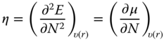 |
|
| Chemical softness, S |  |
|
| Chemical electrophilicity, ω |  |
 |
Chemical potential, μ, which is the negative of electronegativity in the Parr definition [18], measures the escaping tendency of electrons at constant external potential, υ. Chemical hardness, η, captures the resistance of chemical species to electron transfer and is expressed as the second derivative of energy, E, with respect to the number of electrons, N, at constant external potential. Both chemical potential and hardness are related to the ionization potential (IP) and electron affinity (EA), which in turn can be determined using ϵHOMO and ϵLUMO according to Koopman's theorem. Global softness can be expressed as the inverse of chemical hardness; the approximation of softness and hardness using ϵHOMO and ϵLUMO is consistent with the principles of HSAB and FMO theory discussed previously. The electrophilicity index, ω, measures the second-order energy change of an electrophile as it is saturated with electrons [19]. The term “electroaccepting power” is sometimes used [20, 21] and this concept has shown to be useful in understanding electrophilicity of a wide variety of systems [22–24]. Gázquez et al. proposed that the same expression used for “electroaccepting power” can be applied to define “electrodonating power” (or nucleophilicity) of the system. In this case, ![]() , the optimum amount of charge transferred, would be negative when the system is donating charge to the environment (nucleophilicity index) and positive when the system is accepting charge from the environment (electrophilicity index) [21]. Thus, whether or not the system is gaining stability in the electron-transfer process would depend on the difference in the chemical potential of the system and the environment [25].
, the optimum amount of charge transferred, would be negative when the system is donating charge to the environment (nucleophilicity index) and positive when the system is accepting charge from the environment (electrophilicity index) [21]. Thus, whether or not the system is gaining stability in the electron-transfer process would depend on the difference in the chemical potential of the system and the environment [25].
In Table 2.3, four different Michael acceptors, which are soft electrophiles, are shown along with glutathione (GSH)-binding rate constants and global electronic indices calculated from HOMO and LUMO energies at the ![]() level of theory. Organic chemistry principles dictate that the observed trend in reactivity is based on electronic effects: acrylates tend to be less reactive owing to competing resonance, although this effect is reduced by the electron-withdrawing effect of unsaturated
level of theory. Organic chemistry principles dictate that the observed trend in reactivity is based on electronic effects: acrylates tend to be less reactive owing to competing resonance, although this effect is reduced by the electron-withdrawing effect of unsaturated ![]() bonds. Computed molecular electrophilicity and softness indices are generally consistent with this trend, except for the
bonds. Computed molecular electrophilicity and softness indices are generally consistent with this trend, except for the ![]() versus
versus ![]() case. However, when the ϵHOMO of GSH is considered in the calculations of
case. However, when the ϵHOMO of GSH is considered in the calculations of ![]() or
or ![]() , the predicted reactivity trend is consistent with experimental data across the entire series.
, the predicted reactivity trend is consistent with experimental data across the entire series.
Table 2.3 Global electronic parameters for 3-penten-2-one, propargyl acrylate, allyl acrylate, and methyl acrylate derived from HOMO and LUMO energies at the mPW1PW91/MIDIX + level of theory
 |
 |
 |
 |
|
| Exptl log kGSH (L/mol/min) | 3.10 | 1.71 | 1.29 | 1.06 |
| Chemical electrophilicity, ω (eV) | 1.90 | 1.88 | 1.79 | 1.81 |
| Chemical softness, S (eV) | 0.0889 | 0.0771 | 0.0782 | 0.0755 |
| Electrophilicity, ω | 1.88 | 1.79 | 1.72 | 1.71 |
| w/HOMOGSH (eV) | ||||
| Softness, ω | 0.0931 | 0.0910 | 0.0894 | 0.0892 |
| w/HOMOGSH (eV) | ||||
2.6.2 Local (Atom-Based) Electronic Parameters
The value of local descriptors is in describing reactivity in a specific part of the molecule. The endgame is to capture reaction energetics that could be obtained from far more demanding reaction-coordinate modeling using simple and computationally inexpensive calculations of steric and electronic parameters of the toxicant's (and biological target's) ground state(s). This is particularly useful when large databases of compounds need to be screened rapidly for their toxic effects in comparative hazard assessment. While a speedy evaluation of molecular interactions between a xenobiotic and a biological target is possible (e.g., docking as used in computational drug discovery), the method employed is usually too simplistic to allow for reliable comparative assessment, particularly when covalent interactions are involved [26]. To this end, using local descriptors offers an alternative approach, which may take advantage of higher level of theory at the expense of model size. The list below is by no means exhaustive, but simply offers a few examples that have found use in predictive toxicology.
2.6.2.1 Parameters Derived from Frontier Molecular Orbitals (FMOs)
Local (atom-based) analogs of global electronic parameters can be derived to help define the preferred site for a chemical reaction in a molecule and/or to compare relativities of two or more structurally similar compounds. Some of these local electronic parameters are outlined in Table 2.4, as rationalized within the framework of density functional theory [27]. Local hardness is omitted from Table 2.4 as it contains information already provided by local softness. To evaluate local softness and electrophilicity, a Fukui function is defined in the first row of Table 2.4. A Fukui function is a normalized function that measures the propensity of a reactant to accept or donate electrons from or to another chemical system. Since for a molecular system the derivative of electron density, ρ, with respect to the number of electrons is discontinuous, the Fukui function has different formalisms for electrophilic ![]() and nucleophilic
and nucleophilic ![]() attacks on a molecule. From Table 2.4, N refers to the closed-shell system, whereas
attacks on a molecule. From Table 2.4, N refers to the closed-shell system, whereas ![]() and
and ![]() refer to the system with an added and removed electron, respectively. On the basis of the work of Yang and Mortier [28], a Fukui function condensed to atoms can be evaluated through integration over atomic regions using population analysis. To this end,
refer to the system with an added and removed electron, respectively. On the basis of the work of Yang and Mortier [28], a Fukui function condensed to atoms can be evaluated through integration over atomic regions using population analysis. To this end, ![]() and
and ![]() on a particular atom (sometimes referred to as the Fukui index) can be calculated using partial atomic charges. Although omitted from Table 2.3 for brevity, local softness and electrophilicity can also be expressed in terms of condensed Fukui functions.
on a particular atom (sometimes referred to as the Fukui index) can be calculated using partial atomic charges. Although omitted from Table 2.3 for brevity, local softness and electrophilicity can also be expressed in terms of condensed Fukui functions.
Table 2.4 Local electronic parameters derived from density functional theory
| Fukui function, f(r) | 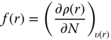 |
 |
 |
||
| Local softness, s(r) |  |
 |
| Local electrophilicity, ω(r) |  |
|
The quantitative interpretation of local electronic parameters has been debated upon for many years. It is agreed that local softness and hardness provide pointwise measures of the localized concentration of the corresponding global parameter [27]. From a local extension of the HSAB principle, it can be stipulated that the preferred site of the molecule to react in an orbital-controlled interaction is the region characterized by the maximum in the Fukui function. Conversely, if a reaction is charge-controlled (i.e., ionic reactions), it cannot be described by local hardness as the HSAB principle does not consider electrostatic effects. One should also be cautious in making extensive comparisons between different sites within the same molecule and across different molecules. Torrent-Sucarrat et al. recommend that only atoms with distinctively high softness/hardness within a molecule be used in comparisons to other atoms in the same or other molecules [27]. In other words, one cannot draw conclusions from small differences and small values because in those cases local softness/hardness only represents the atomic contribution to the global parameter.
Local electronic parameters have found use in predicting chemical reactivity in toxicity pathways. For example, Wondrousch et al., showed that the local electrophilicity index can be employed as a predictor of binding rates of Michael acceptors to GSH, outperforming global electrophilicity [29, 30].
The utility of condensed-to-atoms Fukui functions is shown in Figure 2.4. In Figure 2.4a, the four α, β-unsaturated carbonyls are soft electrophiles and known skin sensitizers [31]. The maxima in ![]() of the four compounds are consistent with the preferred sites of attack by skin protein nucleophiles [32]. While the haptenation mechanism for compounds 1, 3, and 4 is 1,4-(Michael) addition, 1,2-addition (Schiff-base formation) is favored for compound 2 owing to steric hindrance of the γ-carbon. Therefore, the electronic effect of the methyl substituents effectively replaces their steric significance. When multiple 1,4-additions are possible (compounds 3 and 4), the less hindered site is identified correctly in each case. For 4, an alternate approach is provided in Figure 2.4b by considering the atomic contributions to the LUMO orbital in the LCAO-MO (molecular orbital represented as a linear combination of atomic orbitals) method (see Table 2.4); the largest coefficients suggest preferred attack sites. Fukui indices can be used to guide transition-state calculations; free energies of activation were briefly considered here at the attack sites suggested by Fukui indices. Calculated with the PM6 method, the low barrier indicates higher reactivity for compound 1 than for 2, 3, and 4, which is consistent with higher sensitization potential for 1, as determined from local lymph node assays (LLNAs) [31].
of the four compounds are consistent with the preferred sites of attack by skin protein nucleophiles [32]. While the haptenation mechanism for compounds 1, 3, and 4 is 1,4-(Michael) addition, 1,2-addition (Schiff-base formation) is favored for compound 2 owing to steric hindrance of the γ-carbon. Therefore, the electronic effect of the methyl substituents effectively replaces their steric significance. When multiple 1,4-additions are possible (compounds 3 and 4), the less hindered site is identified correctly in each case. For 4, an alternate approach is provided in Figure 2.4b by considering the atomic contributions to the LUMO orbital in the LCAO-MO (molecular orbital represented as a linear combination of atomic orbitals) method (see Table 2.4); the largest coefficients suggest preferred attack sites. Fukui indices can be used to guide transition-state calculations; free energies of activation were briefly considered here at the attack sites suggested by Fukui indices. Calculated with the PM6 method, the low barrier indicates higher reactivity for compound 1 than for 2, 3, and 4, which is consistent with higher sensitization potential for 1, as determined from local lymph node assays (LLNAs) [31].

Figure 2.4 (a) Fukui indices, f+, computed for 4α,β-unsaturated carbonyls using Hirshfeld charges at the mPW1PW91/MIDIX+ level of theory. Maxima in the Fukui function are labeled with a black dot and a corresponding value; black circles mark the next highest values. Free energies of activation were calculated with the PM6 semiempirical method in the gas phase. Sensitization potential categories were derived from LLNA EC3% values [31]. (b) The LUMO orbital for 4.
2.6.2.2 Partial Atomic Charges
Partial atomic charges are not only useful in determining Fukui indices; they can be used directly as descriptors of intra- and intermolecular electrostatic interactions. Many methodologies have been formulated to compute partial charges, which can be divided into four classes, I–IV. Class I charges are calculated using classical models of dipoles or are derived directly from experimental data. Partial equalization of orbital electronegativity is an exemplary method implemented by Gasteiger and Marsilli [33]. The advantage of Class I charges is high computational speed and so they are best applicable for quick assessments of large datasets of compounds. Class II charges involve direct partitioning of the molecular wave function or electron charge density into atomic contributions. The most popular schemes are Mulliken, Löwdin, natural charges (natural population analysis (NPA)) and Hirshfeld charges. From a practical perspective, Hirshfeld charges are perhaps the least sensitive to basis set size or choice of basis within this group [34]. Class III charges are determined from analysis of physical observables, which are calculated from the molecular wavefunction. The most prominent examples include CHarges from ELectrostatic Potentials using a Grid based method (CHELPG) and Merz-Kollman (MK) charge schemes, which are both derived from a molecular ESP (ESP, Section 2.6.1.1). Being derived from molecular ESP, CHELPG, and MK charges are useful in characterizing intermolecular short- and long-range electrostatic interactions. Their biggest drawback is in computing partial charges for atoms not on the molecular surface. Influenced by molecular conformations, partial charges for “buried” atoms can vary widely even if the ESP is insensitive to these conformational changes. To this end, prediction of intramolecular interactions using ESP charges can be questionable. Lastly, class IV charges are derived by a semiempirical mapping of a precursor charge of type II or III to reproduce experimentally determined observables such as dipole moments. The CM (Charge Model) 1–5 are good examples, and currently available to the user in various software packages, such as Gaussian or GAMESS. CM5 charges, derived from Hirshfeld population analysis, show high accuracy across different chemical classes and remarkable independence of the level of theory used, and thus can be generally recommended [34].
2.6.2.3 Hydrogen-Bonding Interactions
Hydrogen bonds are quintessential in biochemistry. Proteins and nucleic acids are composed of numerous NH2 and OH groups that can donate hydrogen bonds and ![]() groups that can accept them. To this end, hydrogen bonds guide the shape and function of biomolecules. They are also important in enzymatic catalysis to stabilize a ligand in a binding pocket. Hydrogen bonds can be used as descriptors either by counting atomic donor and acceptor sites or by assessing the “actual” number and energetics of the hydrogen bonds formed in molecular simulations. In statistical mechanics, one can compute radial distribution functions which provide the normalized probability of having one molecule a given distance from another molecule – such interaction can be reflective of hydrogen bonding, in which case integration of these functions yields the number of hydrogen bonds present. Additionally, energy pair distributions can be calculated, which record the average number of molecules that interact with the system in question and their corresponding energies. It is important to note that while hydrogen bonding is mostly electrostatic in nature and can therefore be represented by the Coulomb potential between two atom-based charges, very strong hydrogen bonds have some orbital character. For those systems, high-level quantum mechanical calculations should be used to provide accurate results.
groups that can accept them. To this end, hydrogen bonds guide the shape and function of biomolecules. They are also important in enzymatic catalysis to stabilize a ligand in a binding pocket. Hydrogen bonds can be used as descriptors either by counting atomic donor and acceptor sites or by assessing the “actual” number and energetics of the hydrogen bonds formed in molecular simulations. In statistical mechanics, one can compute radial distribution functions which provide the normalized probability of having one molecule a given distance from another molecule – such interaction can be reflective of hydrogen bonding, in which case integration of these functions yields the number of hydrogen bonds present. Additionally, energy pair distributions can be calculated, which record the average number of molecules that interact with the system in question and their corresponding energies. It is important to note that while hydrogen bonding is mostly electrostatic in nature and can therefore be represented by the Coulomb potential between two atom-based charges, very strong hydrogen bonds have some orbital character. For those systems, high-level quantum mechanical calculations should be used to provide accurate results.
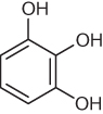
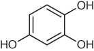
The utility of predicting the number and strength of hydrogen-bonding interactions in aqueous medium as a metric of human skin permeability is illustrated on three phenols in Table 2.5. The well-known corrosiveness of these phenols can affect permeability rates; therefore, short duration of the test and very low concentrations are key to preserving the stratum corneum intact and providing meaningful metrics. Among the three phenols, the most permeable is 2,4-dichlorophenol, which can only donate and accept one hydrogen bond; Cl⋯H−OH interactions are considerably weaker. 1,2,3-Trihydroxybenzene is more permeable because it can accept and donate nearly three hydrogen bonds; however, its ability to form intramolecular hydrogen bonds reduces bonding to nearby water. 1,2,4-Trihydroxybenzene is the most water soluble and least permeable in the series as its substitution pattern accommodates surrounding water molecules more effectively than 1,2,3-trihydroxybenzene. Computed energies of the intermolecular hydrogen bonds for the three compounds (last row in Table 2.5) are consistent with the experimental trend in skin permeability; the more favorable the interaction with water, the less permeable the compound. Note that the molecular dipole, a metric frequently used to inform solubility in polar medium, does not underline the trend in skin permeability for this series.
Table 2.5 Hydrogen bonding (HB) as an inverse metric of human skin permeability
 |
 |
 |
|
| Experimental log KP (cm/s) | |
|
|
| HB donors/acceptors | 1.0/1.0 | 2.8/2.8 | 2.9/3.3 |
| Interaction energies (kcal/mol) | |||
| Dipole (D) | 2.5 | 2.3 | 3.5 |
Skin permeability values were determined from in vitro studies [35]; hydrogen bonds and molecular dipole moments were calculated from MC simulations utilizing CM1A charges on the solute and TIP4P water model, averaged over ![]() configurations. A cutoff of
configurations. A cutoff of ![]() was used to specify hydrogen bonding in energy pair distributions.
was used to specify hydrogen bonding in energy pair distributions.
2.6.2.4 Bond Enthalpies
This section segues into an ensuing discussion of descriptors derived from explicit interactions of two or more chemicals. Thus far we have largely sidelined radical chemistry, although Fukui functions, for example, can be derived for a radical attack on a molecule [36]. Bond dissociation energy (BDE) describes the enthalpy change for a homolytic cleavage of a chemical bond, that is, separation into free radicals. Understanding how readily molecules cleave their bonds to form free radicals is important to redox cycling. For example, the metabolism of quinone-like compounds involves enzymatic reduction by one or two electrons to form the corresponding semiquinone or hydroquinone, respectively. In the reverse process, the hydroquinone and semiquinone can be oxidized by molecular oxygen, generating a superoxide radical anion, which triggers production of other reactive oxygen species that can lead to oxidative stress [37].
Two antioxidants, hydroquinone (HQ) and t-butyl hydroquinone (tBHQ), were contrasted in their ability to undergo oxidation to the corresponding quinones using bond dissociation energies (Figure 2.5). Since tBHQ is an asymmetric molecule, two oxidation pathways are possible. The calculations suggest that oxidation of tBHQ is more facile than that of HQ. The difference in bond dissociation energies is about 2.5 kcal/mol, favoring tBHQ. The calculations shown in Figure 2.5 were performed at the ![]() level of theory in the gas phase.
level of theory in the gas phase.

Figure 2.5 Two-electron oxidation of hydroquinone (HQ) and t-butyl hydroquinone (tBHQ) to quinones, calculated at the M06-HF/6-31+G(d) level of theory in the gas phase. The solid black line represents energy difference between the HQ and tBHQ pathways, each recorded relative to enthalpies of the fully reduced HQ and tBHQ, respectively. The gray line represents the difference between the HQ pathway and the energetically less favorable tBHQ pathway. Each specie considered in the oxidation process is recorded below the graph with t-butyl substituents omitted for clarity. The species resulting from superoxide radical anion generation, phenoxy radical, and quinone are about 2.5 and 2.7 kcal/mol lower in energy in the (major) tBHQ than in the HQ pathway.
2.6.3 Modeling Chemical Reactions
In the previous section, the first step toward considering the biological target was to observe how the toxicant responds when an electron is added to or removed from its molecular wavefunction. The next step might be to include an atomistic yet highly reduced representation of the target, focusing on the chemical region of interest. Modeling chemical reactions translates to computing the energy profile of a reaction along its reaction coordinate(s). A detailed outline of the pathway is not always necessary; analysis of the reactant and product minima is sufficient to reveal reaction thermodynamics, that is, the favorability of a reaction to proceed toward products. Moreover, kinetic feasibility can be gauged by calculating transition-state energetics, although these calculations are far more difficult and resource intensive. In practice, a series of educated guesses for minima and saddle points along the reaction coordinate can save computational time. Even then, in order to include covalent reactivity in descriptor calculations, a substantially reduced form of the biological target (and possibly the toxicant as well) is necessary to assess reaction energetics with adequate level of theory and obtain results in reasonable time frames. To consider electrostatic effects of the medium surrounding the reactive centers, a hybrid QM/MM description of the system can be used.
The calculation of transition states deserves further discussion. A transition state refers to a surface around a transition structure, the highest point on the minimum energy path that connects reactants to products on the free energy surface of the reacting system, that is, the reaction coordinate (RC). A free energy surface can be analyzed using a sampling method; however, as this is a computationally demanding exercise for QM or QM/MM calculations, a geometry minimization algorithm is often used instead to locate the highest saddle point along the RC. This state is characterized by a single imaginary frequency corresponding to a normal mode of the reaction coordinate. For geometry minimizations, following the reaction coordinate in the forward (i.e., toward products) and reverse (i.e., toward reactants) directions from the transition structure is often crucial to verifying that the desired transition structure was in fact found. Reduced to a stationary point, a transition structure that appears to have the correct geometry may correspond to a different process than the one of interest. The notion that a transition state allows for a population of molecules, that is, that some variation in degrees of freedom other than the reaction coordinate is permitted, is important to transition state theory.
Equation (2.7) is a frequently used expression of the transition state theory, which relates activation free energy, ΔG≠, to the rate constant of a unimolecular reaction. Transition state theory supposes that an equilibrium exists between the transition state and the reactants, and hence assumes population distribution of both states. In practice, ΔG≠ is calculated as the difference in free energy between the transition state and the reactants, ![]() , where
, where ![]() where U0 is the internal energy at 0 K and Q is the partition function.
where U0 is the internal energy at 0 K and Q is the partition function.
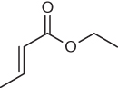
The ability to accurately calculate reaction rates is very important in toxicology. Mulliner et al. showed that calculated reaction barriers can be used to predict log kGSH in screening for electrophilicity-driven toxicity of α, β-unsaturated carbonyls [38]. Table 2.6 illustrates four different Michael acceptors for which calculated barriers underline the observed trends in reaction kinetics.
Table 2.6 Reaction barriers correlated to GSH-binding rate constants for methylacrolein, 3-penten-2-one, allyl acrylate, and ethyl crotonate
 |
 |
 |
 |
|
| Exptl log kGSH (L/mol/min) |
2.31 | 1.43 | 1.29 | |
| ΔE≠ (kJ/mol) | 29.6 | 67.5 | 72.2 | 103.2 |
Reaction barriers were calculated at the B3LYP/6-31G(d,p) level of theory using methane thiol as a model nucleophile [38].
In a different study, Kostal et al. examined the relevance of computed free energies of activation and reaction on the mutagenicity potential of simple epoxides [39]. The study assumed that all compounds were readily bioavailable, and that the chloride anion could be used as a model for DNA nucleotides given comparable nucleophilic strength. The study found that a cutoff value in free energies of reaction effectively separated mutagens from non-mutagens for the series of compounds considered. More recently, Zhang et al. investigated a diverse set of aliphatic epoxides, substituted styrene epoxides, and PAH epoxides using DFT calculations [40]. Activation energies for SN2 reactions between the epoxides and the guanine N7 site were well-correlated with the epoxides' mutagenic potential; expectedly, higher mutagenic activity was associated with lower activation energies.
Table 2.7 briefly illustrates how reaction energetics can be used to distinguish mutagenic from non-mutagenic epoxides in a simple substitution series. In this series, the mutagens have noticeably smaller free activation energies and formation of the corresponding alcohol is thermodynamically more favorable. Since reaction occurs on the less-substituted carbon, it is the electrostatic repulsion between the halogen and the incoming nucleophile that accounts for lower reactivity of the 2,3-substituted epoxides.
Table 2.7 Reaction energetics as a predictor of mutagenicity potentials for 2,2-difluorooxirane, 2,2-dichlorooxirane, 2,3-dichlorooxirane, and 2,2,3-trichlorooxirane
 |
 |
 |
 |
|
| Mutagenic potential | + | |||
| ΔG≠ (kcal/mol) | 12.2 | 16.3 | 28.0 | 21.1 |
| ΔG (kcal/mol) |
All values were calculated at the ![]() level of theory in aqueous solution using a continuum solvation model, IEF-PCM [39].
level of theory in aqueous solution using a continuum solvation model, IEF-PCM [39].
Free energy changes associated with a reaction coordinate can sometimes be predicted using carefully chosen electronic parameters and physicochemical properties derived from ground-state structures. Figure 2.6 illustrates this approach for a series of skin-sensitizing chemicals that undergo haptenation with skin proteins via the nucleophilic substitution mechanism (SN2) [41]. This approach is considerably less demanding than reaction pathway modeling and may be preferable when accuracy is of lesser concern than the ability to process compounds automatically (i.e., with minimal expert intervention) and fast.

Figure 2.6 Linear models for free activation energies (a) and free energies of reaction (b) for nucleophilic substitutions of halides, epoxides, and tosylates; ΔG† and ΔGrxn values were computed in aqueous solution at the M06-2X/6-311 + G(d,p) level of theory; ΔG≠ = 1706.38sα − 27.26EE − 243.69S − 1.76SASAα + 35.72(S × SASAα) − 4.02; N = 15; R2 = 0.98;  = 0.97; RMS = 0.96. ΔGrxn = 801.01sα − 4.12 μ + 8.90SASAα + 2.04(μ × SASAα) − 70.04; N = 15; R2 = 0.95;
  = 0.93; RMS = 0.35. sβ = local softness on the α carbon; EE = electrostatic solvation energy; S = global softness; SASAα = surface accessible solvent area on the α carbon; μ = chemical potential [41].
2.6.4 QM/MM Calculations of Covalent Host-Guest Interactions
Consideration of the entire (or substantial part of the) biological target is rarely a sound strategy in predictive toxicology using QM calculations, even when the nonreactive regions are described classically (i.e., QM/MM calculations). This is due to the enormous number of degrees of freedom that need to be sampled in MC or MD simulations to study reaction free energy surfaces. That being said, such approaches are sometimes used in computational chemistry to study enzymatic reactions involving a single or relatively few ligands. Such calculations are rigorous enough to elucidate or propose novel chemical mechanisms, but are too resource intensive to carry out in the context of typical hazard assessments. To this end, one could envision restrained use of these calculations to fill in data gaps in molecular mechanisms of toxicity for a class of chemicals. Since to the best of our knowledge, these calculations have not yet been employed in toxicology and no suitable examples exist, the approach is demonstrated using our recent study of the tautomerization mechanism in the microphage migration inhibitory factor (MIF).
MIF is a critical upstream regulatory protein of the innate and acquired immune response. It is a keto-enol tautomerase capable of shifting the equilibrium from keto to the enol form for a host of substrates, such as dopachrome [42] and p-hydroxyphenylpyruvate (HPP) [43, 44]. HPP is an intermediate in the metabolism of phenylalanine, the aromatic side chain of which is hydroxylated to form tyrosine. In HPP tautomerization, it is expected that both a general acid and a base are involved. Preceding our investigation, the catalytic role of a nearby proline residue (Pro1) as a general base has been demonstrated by several experimental studies (Figure 2.7) [45–48]. However, the identity of the catalytic acid was not known, although proximal residues Tyr95 or Lys32 have been suspected in other studies (Figure 2.7). Our computational exploration of the dynamics of the bound HPP substrate revealed that Tyr95 and Lys32 are either not positioned well to donate a proton to the substrate or their calculated pKa's suggest this is not a favorable process (Figure 2.7a). However, we observed that there are two proximal residues changing ionization state in the pH range 5–9, Pro1 and His62. Of these two, it is unlikely that His62 plays any role in the MIF catalytic mechanism as the MIF mutant, His62T, possesses the same catalytic efficiency as the wild-type [49]. Thus, our focus shifted to Pro1 as both a potential catalytic base and acid.
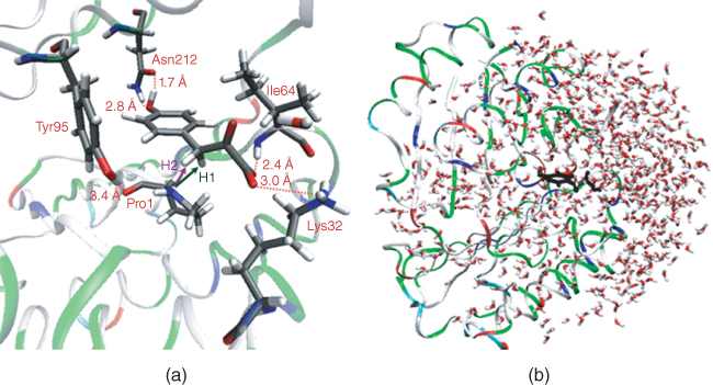
Figure 2.7 (a) Active site of MIF (1CA7) with bound HPP in the keto form from QM/MM/MC simulations. (b)Truncated MIF–HPP complex with about 680 water molecules; the ligand is marked in black.
Computationally, this system's reaction free energy surface can be studied using free energy perturbation (FEP) calculations in conjunction with MC simulations (MC/FEP). In practical terms, reaction coordinates are gradually incremented while all other internal degrees of freedom are sampled at every step. To reduce cost, the QM region only involved the substrate and side chains of the key residues in the binding pocket, totaling 83 heavy atoms; the rest of the system (Figure 2.7b) was treated classically with the optimized potentials for liquid simulations (all-atom) (OPLS-AA) force field. To further reduce cost, an inexpensive semiempirical method (Pairwise distance directed gaussian modification of the parametrized model number 3 (PDDG/PM3)) was used. Even then, to analyze a single proton transfer involved in the keto-enol tautomerization required about 18 billion calculations. A sample of a reaction free energy surface describing a proton transfer from Pro1 to HPP to yield the enolate is shown in Figure 2.8.

Figure 2.8 (a) Computed 2D free energy map for the H2 proton transfer (see Figure 2.7). The white dashed line follows the minimum free energy path. (b) Snapshots of the transition state (TS) and the enolate intermediate illustrating relevant electrostatic interactions. The resolution based on a single FEP window is 0.025 Å.
Our study found that a proton transfer from HPP to Pro1 yielded an enolate intermediate that was well-positioned to be re-protonated on the oxygen by Pro1. Furthermore, this process was found to be kinetically most favorable and corresponded to an overall free energy change in agreement with experimental results. One could envision how this computational approach is applied to computational toxicology to fill mechanistic data gaps in key toxicodynamics phenomena. If a molecular mechanism is elucidated for a chemical class, then more simplistic methods, such as those illustrated in previous sections of this chapter, could be applied within that chemical class to screen new compounds for interactions with the biological target.
2.6.5 Medium Effects and Hydration Models
Including a solvent in a computational model effectively increases system size. Solvation can be considered in all models described above: a single structure used to calculate physicochemical properties or a model that considers electrostatic or covalent interaction between multiple structures. Solvation affects electronic distribution in a molecule, altering electronic properties such as orbital energies, partial atomic charges, dipole moments, as well as molecular volume and accessible surface area by perturbing conformational equilibria. Processes in solution can be viewed as occurring on a lower free-energy surface than equivalent gas-based transformations. Since any chemical process takes place between minima on the free energy surface, if these states are characterized by differential solvation then the process will have a different equilibrium constant in solution than in the gas phase. The same applies to transition states; a transition structure may be more or less well solvated than the reactant(s), implying smaller or larger free energy of activation than a corresponding gas-phase process. Many examples of this phenomenon are known. For the tautomeric equilibrium between 4-hydroxypyridine and 4-pyridone, aqueous solvation changes the equilibrium constant by some six orders of magnitude [50]. In epoxide-forming cyclization reactions, solvation can drastically alter reaction rates depending on the ring substitutions [7]. Perhaps the most studied example is a nucleophilic substitution reaction between a chloride ion and methyl chloride. While the gas-phase activation free energy is about 3 kcal/mol, the diffuse negative charge associated with the transition structure compared to a chloride ion leads to preferential solvation of the reactants, and the rate in solution decreases by more than 15 orders of magnitude [51]. Despite these and many other solvent effects documented in the literature, gas-phase conditions are typically invoked in predictive modeling in toxicology owing to lower computational cost.
In computational models, the solvent can be represented either implicitly or explicitly. For implicit models, the charge distribution of the solvent around the solute is replaced by a continuous electric field that represents a statistical average over all solvent degrees of freedom at thermal equilibrium. Generalized Born/surface area (GB/SA), polarizable continuum models (PCM) and the universal solvation model based on solute electron density (SMD) are frequently used examples. Performance of implicit solvation models varies. For neutral compounds, carefully parameterized models exhibit average errors over large datasets on the order of about 0.5 kcal/mol. A single-charged species ![]() poses more difficulties experimentally, and solvation free energies are accurate to about
poses more difficulties experimentally, and solvation free energies are accurate to about ![]() . Reliable data for species of higher charge are extremely scarce, so no valid comparison can be made.
. Reliable data for species of higher charge are extremely scarce, so no valid comparison can be made.
The effect of solvation on calculated energetics is demonstrated in Table 2.8. Three benzyl halide skin sensitizers, 1-chloromethylpyrene (1), 4-nitrobenzyl bromide (2), and benzyl bromide (3) were compared in their propensity to react with cysteine residues of the Keap1 protein via SN2 mechanism. Free energies of activation and reaction were calculated both in the gas phase and in aqueous solution using a polarizable continuum model (IEF-PCM) at the ![]() level of theory. Table 2.8 shows lower barrier and more negative free energies for 2 and 3 than 1 in both gas phase and in solution, consistent with the fact that bromide is a better leaving group than chloride. In examining solvent effects, free activation energies increase owing to more favorable solvation of charge-localized reactants than charge-diffuse transition structures. Furthermore, 2 is kinetically favored in the gas phase, while 3 is favored in solution; the difference is considerable, about 16 kcal/mol. It can be proposed that the electron-withdrawing effect of the para-nitro group is more pronounced in solution than in the gas phase as increased charge separation is favored in a polar solvent. As it is a resonance withdrawing effect, the charge on the methylene carbon is made more negative by this effect (
level of theory. Table 2.8 shows lower barrier and more negative free energies for 2 and 3 than 1 in both gas phase and in solution, consistent with the fact that bromide is a better leaving group than chloride. In examining solvent effects, free activation energies increase owing to more favorable solvation of charge-localized reactants than charge-diffuse transition structures. Furthermore, 2 is kinetically favored in the gas phase, while 3 is favored in solution; the difference is considerable, about 16 kcal/mol. It can be proposed that the electron-withdrawing effect of the para-nitro group is more pronounced in solution than in the gas phase as increased charge separation is favored in a polar solvent. As it is a resonance withdrawing effect, the charge on the methylene carbon is made more negative by this effect (![]() vs
vs ![]() from Mulliken population analysis). Thus, the attack of the negatively charged nucleophile is less favorable on 4-nitrobenzyl bromide in aqueous solution. Note that neither gas nor aqueous phase reaction energies underline the differences in sensitization potency between 1, 2, and 3 [32]. Skin permeability is an important factor and would need to be considered alongside reaction energetics if a predictive model were to be developed.
from Mulliken population analysis). Thus, the attack of the negatively charged nucleophile is less favorable on 4-nitrobenzyl bromide in aqueous solution. Note that neither gas nor aqueous phase reaction energies underline the differences in sensitization potency between 1, 2, and 3 [32]. Skin permeability is an important factor and would need to be considered alongside reaction energetics if a predictive model were to be developed.
Table 2.8 Reaction energetics computed for three benzyl halide skin sensitizers at the M06-2X/6-311 + G(d, p) level in gas phase and in aqueous solution
 1 1 |
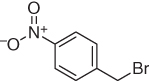 2 2 |
 3 3 |
|
| Sensitization potential | Extreme | Extreme | Strong |
| ΔG≠, gas (kcal/mol) | |
|
|
| ΔG≠, aq (kcal/mol) | 16.2 | 13.3 | 7.5 |
| ΔG, gas (kcal/mol) | |||
| ΔG, aq (kcal/mol) |
Methyl thiolate was used as a model nucleophile; polarizable continuum model (IEF-PCM) was used to model aqueous environment. Sensitization potency category was determined from LLNA EC3% values [32].
A computationally more demanding alternative to implicit representation of the solvent is to include solvent molecules in the model explicitly. Explicit models are needed when knowledge of the explicit behavior of the surroundings is deemed to be important; the perfect example was presented in Section 2.6.2.3, where MC simulations of substituted phenols in aqueous solution were used to assess hydrogen bonding between the solutes and the solvent as a measure of skin permeability. The downside of explicit models is greater computational cost – explicit representation of a condensed phase leads to a system characterized by enormous number of degrees of freedom. Properties of such systems must be determined as statistical averages over phase space, as discussed in Section 2.5. To reduce computational costs, simple atomistic representations of the solvent are usually adopted, the simplest being an MM model.
2.7 Rational Design of Safer Chemicals
Thus far we have considered computational chemistry techniques that can be applied to solve problems in predictive toxicology, whether to screen chemicals for their hazard or to fill mechanistic data gaps in toxicity pathways. Predicting toxicity of existing chemicals is fundamentally different from designing new molecules that fulfill certain functions yet have minimal biological activity.
Given the complexity of biochemical pathways in any target species, our limited understanding of these pathways, limited resources, and the far-reaching connotation of “chemical safety,” two approaches can be postulated: a nonspecific approach that considers elements of bioavailability and reactivity broadly to cover multiple endpoints and modes of action, and a highly refined approach that focuses on one type of molecular event. An example of the former was published by Voutchkova et al. and Kostal et al., who developed design guidelines for chemicals with minimal acute and chronic aquatic toxicity using just two properties: the octanol-water partition/distribution coefficient (log P/D) and the HOMO-LUMO gap (Δϵ) [14, 15]. These properties were used to demarcate a “safer chemical space”; any existing or newly designed chemical that falls within this space was postulated to be about 10 times more likely to have low aquatic toxicity than chemicals that do not meet the criteria (Figure 2.9).

Figure 2.9 Scatter plots of the octanol-water partition and distribution coefficients (log P and log D) versus HOMO-LUMO gap (Δϵ) calculated at the mPW1PW91/MIDIX+ level of theory. The 500+ compounds represented are colored by category of concern for acute aquatic toxicity (red = high concern; orange = medium concern; yellow = low concern; green = no concern) based on a 96-h toxicity assay of the fathead minnow [14]. The highlighted upper-left quadrant marks the “safer chemical space” (log P/D < 1.7; Δϵ > 6 eV), which should be targeted in designing new molecules.
Source: Adapted from Kostal et al. 2015 [14].
Since log P, log D, and Δϵ can be related to molecular structure, they can also be used qualitatively as design guidelines for developing new chemicals without carrying out calculations. While basic principles of organic chemistry can be applied to infer the degree of lipophilicity versus hydrophilicity from a chemical structure (as reflected in log P or D), correlation between Δϵ and structure is harder to understand. Larger Δϵ is generally associated with more stable molecules; a molecule trapped in a deep well on a free energy surface will be both thermodynamically and kinetically stable. Ruiz-Morales investigated polycyclic aromatic hydrocarbons (PAHs), which are potential carcinogens, and their fluorescence emission spectra to draw links between molecular size, structure, and the band gap, Δϵ [52]. The band gap was found to increase going from linear arrangement to the most compact structure, which also increased the number of localized resonant sextets. PAHs with zigzag structures and full resonance had the largest Δϵ values, making them thermodynamically and kinetically stable. Stable PAHs are less likely to undergo metabolic oxidation to become potent carcinogens. The results were extrapolated to the fused aromatic ring region in asphaltenes, experimental Δϵ values of which were obtained from fluorescence emission data, and were compared with the calculated Δϵ values of free PAHs.
Note that the design guidelines described in Figure 2.9 omitted function as a design criterion. In a recent study, Burello proposed a computational screening approach to design safer nanomaterials that considers both toxicity and functionality [53]. The work was based on the calculation of key physicochemical properties of nanomaterials. Some were related to inhalation toxicity (size, conduction band energy, charge, and solubility), and others to functionality (band gap, transmittance). These properties were proposed as a screening tool to select a pool of candidates for further experimental testing and development.
For broad design rules, functional requirements may easily overlap with safety requirements. In a trivial example, consider a chemical that needs to be reactive in a certain species to function (e.g., an insecticide) but should not be reactive in other species. To this end, there is value in highly refined design approaches that can distinguish between two very similar biological targets. Such approach should, for example, distinguish between a chemical covalently interacting with an insect acetylcholinesterase and a mammal variant of this enzyme. Free energy perturbation calculations noted in Section 2.6.4 as means to study mechanisms of complex enzymatic reactions can also be used to capture such minute differences in free energies of binding. For noncovalent host-guest interactions, this process becomes much more computationally feasible as the entire system can be described classically. In an FEP calculation, the free energy associated with perturbing a state A of a system into state B is related to an average of a function of their energy difference evaluated by sampling for state A in the Zwanzig equation (Equation (2.8)).

From Equation (8), states A and B may be different atoms or molecules in a classical treatment, in which case ΔG obtained is for mutating one molecule (or part of a molecule) into another, or they may correspond to different geometries of a molecule in a quantum-mechanical treatment, in which case a free energy map is generated along one or more reaction coordinates (see Section 2.6.4). Among the numerous existing applications of free energy perturbation calculations, the most prominent one is lead optimization of inhibitors in computer-guided drug discovery. In a recent study, which could in future find its analog in predictive toxicology, Cole et al. used FEP calculations in conjunction with MC and MD simulations to investigate binding of benzyloxazole inhibitors to both the wild-type and the Y181C variant of the drug target HIV-RT (Figure 2.10) [54].

Figure 2.10 Benzyloxazole molecule used in the FEP study by Cole et al. [54] and Bollini et al. [55]. The R group was iteratively modified to optimize binding affinity toward HIV-RT.
Source: Adapted from Cole et al. 2015 [54] and Bollini et al. 2013 [55].
In their study, tyrosine to cysteine change in the binding pocket introduced a hydrophobic cavity, which preferred bulky nonpolar substituents on the benzyloxazole. Iterative mutations of the substituents according to Equation (8) revealed the most favorable free energy of binding for isopropyl and ethyl substituents. This result was confirmed with experimental studies that showed sub-10 nM potency for either substituent against both viral strains; by comparison, a methyl analog had a potency by about two orders of magnitude lower [55]. It is not difficult to envision that a similar approach could be applied to minimize activity against a specific biological target. In conjunction with broader design rules, such approach might offer viable strategy for the design of safer chemicals.
References
- 1 Hohenberg, P. and Kohn, W. (1964) Inhomogeneous electron gas. Phys. Rev. B, 136, B864–B871.
- 2 Kohn, W. and Sham, L.J. (1965) Self-consistent equations including exchange and correlation effects. Phys. Rev., 140 (4A), A1133–A1138.
- 3 Goerigk, L. and Grimme, S. (2011) A thorough benchmark of density functional methods for general main group thermochemistry, kinetics, and noncovalent interactions. Phys. Chem. Chem. Phys., 13 (14), 6670–6688.
- 4 Korth, M. and Thiel, W. (2011) Benchmarking semiempirical methods for thermochemistry, kinetics, and noncovalent interactions: OMx methods are almost as accurate and robust as DFT-GGA methods for organic molecules. J. Chem. Theory Comput., 7 (9), 2929–2936.
- 5 Zhan, C.-G., Nichols, J.A., and Dixon, D.A. (2003) Ionization potential, electron affinity, electronegativity, hardness, and electron excitation energy: molecular properties from density functional theory orbital energies. J. Phys. Chem. A, 107 (20), 4184–4195.
- 6 Lynch, B.J. and Truhlar, D.G. (2004) Small basis sets for calculations of barrier heights, energies of reaction, electron affinities, geometries, and dipole moments. Theor. Chem. Acc., 111 (2), 335–344.
- 7 Kostal, J. and Jorgensen, W.L. (2010) Thorpe–Ingold acceleration of oxirane formation is mostly a solvent effect. J. Am. Chem. Soc., 132 (25), 8766–8773.
- 8 Tubert-Brohman, I., Acevedo, O., and Jorgensen, W.L. (2006) Elucidation of hydrolysis mechanisms for fatty acid amide hydrolase and its Lys142Ala variant via QM/MM simulations. J. Am. Chem. Soc., 128 (51), 16904–16913.
- 9 Lu, S.H., Wu, J.W., Liu, H.L. et al. (2011) The discovery of potential acetylcholinesterase inhibitors: a combination of pharmacophore modeling, virtual screening, and molecular docking studies. J. Biomed. Sci., 18, 8–20.
- 10 Piazzi, L., Belluti, F., Bisi, A. et al. (2007) Cholinesterase inhibitors: SAR and enzyme inhibitory activity of 3-[omega-(benzylmethylamino)alkoxy]xanthen-9-ones. Bioorg. Med. Chem., 15 (1), 575–585.
- 11 Piazzi, L., Cavalli, A., Belluti, F. et al. (2007) Extensive SAR and computational studies of 3-{4-[(benzylmethylamino)methyl]phenyl}-6,7-dimethoxy-2H-2-chromenone (AP2238) derivatives. J. Med. Chem., 50 (17), 4250–4254.
- 12 Hansch, C. and Kurup, A. (2003) QSAR of chemical polarizability and nerve toxicity. 2. J. Chem. Inf. Comp. Sci., 43 (5), 1647–1651.
- 13 Fukui, K., Yonezawa, T., and Shingu, H. (1952) A molecular orbital theory of reactivity in aromatic hydrocarbons. J. Chem. Phys., 20 (4), 722–725.
- 14 Kostal, J., Voutchkova-Kostal, A., Anastas, P.T., and Zimmerman, J.B. (2015) Identifying and designing chemicals with minimal acute aquatic toxicity. Proc. Natl. Acad. Sci. USA, 112 (20), 6289–6294.
- 15 Voutchkova-Kostal, A.M., Kostal, J., Connors, K.A. et al. (2012) Towards rational molecular design for reduced chronic aquatic toxicity. Green Chem., 14 (4), 1001–1008.
- 16 Voutchkova, A.M., Kostal, J., Steinfeld, J.B. et al. (2011) Towards rational molecular design: derivation of property guidelines for reduced acute aquatic toxicity. Green Chem., 13 (9), 2373–2379.
- 17 Lopachin, R.M., Gavin, T., Decaprio, A., and Barber, D.S. (2012) Application of the hard and soft, acids and bases (HSAB) theory to toxicant–target interactions. Chem. Res. Toxicol., 25 (2), 239–251.
- 18 Parr, R.G., Donnelly, R.A., Levy, M., and Palke, W.E. (1978) Electronegativity: the density functional viewpoint. J. Chem. Phys., 68 (8), 3801–3807.
- 19 Parr, R.G., Von Szentpaly, L., and Liu, S.B. (1999) Electrophilicity index. J. Am. Chem. Soc., 121 (9), 1922–1924.
- 20 Morell, C., Gazquez, J.L., Vela, A. et al. (2014) Revisiting electroaccepting and electrodonating powers: proposals for local electrophilicity and local nucleophilicity descriptors. Phys. Chem. Chem. Phys., 16 (48), 26832–26842.
- 21 Gazquez, J.L., Cedillo, A., and Vela, A. (2007) Electrodonating and electroaccepting powers. J. Phys. Chem. A, 111 (10), 1966–1970.
- 22 Chattaraj, P.K., Giri, S., and Duley, S. (2011) Update 2 of: electrophilicity index. Chem. Rev., 111 (2), Pr43–Pr75.
- 23 Chattaraj, P.K. and Roy, D.R. (2007) Update 1 of: electrophilicity index. Chem. Rev., 107 (9), Pr46–Pr74.
- 24 Chattaraj, P.K., Sarkar, U., and Roy, D.R. (2006) Electrophilicity index. Chem. Rev., 106 (6), 2065–2091.
- 25 Chamorro, E. and Melin, J. (2015) On the intrinsic reactivity index for electrophilicity/nucleophilicity responses. J. Mol. Model., 21 (3), 53.
- 26 Warren, G.L., Andrews, C.W., Capelli, A.M. et al. (2006) A critical assessment of docking programs and scoring functions. J. Med. Chem., 49 (20), 5912–5931.
- 27 Torrent-Sucarrat, M., De Proft, F., Ayers, P.W., and Geerlings, P. (2010) On the applicability of local softness and hardness. Phys. Chem. Chem. Phys., 12 (5), 1072–1080.
- 28 Yang, W. and Mortier, W.J. (1986) The use of global and local molecular parameters for the analysis of the gas-phase basicity of amines. J. Am. Chem. Soc., 108 (19), 5708–5711.
- 29 Schwobel, J.A.H., Wondrousch, D., Koleva, Y.K. et al. (2010) Prediction of Michael-type acceptor reactivity toward glutathione. Chem. Res. Toxicol., 23 (10), 1576–1585.
- 30 Wondrousch, D., Bohme, A., Thaens, D. et al. (2010) Local electrophilicity predicts the toxicity-relevant reactivity of Michael acceptors. J. Phys. Chem. Lett., 1 (10), 1605–1610.
- 31 Gerberick, G.F., Ryan, C.A., Kern, P.S. et al. (2005) Compilation of historical local lymph node data for evaluation of skin sensitization alternative methods. Dermatitis, 16 (4), 157–202.
- 32 Roberts, D.W., Patlewicz, G., Kern, P.S. et al. (2007) Mechanistic applicability domain classification of a local lymph node assay dataset for skin sensitization. Chem. Res. Toxicol., 20 (7), 1019–1030.
- 33 Gasteiger, J. and Marsili, M. (1980) Iterative partial equalization of orbital electronegativity – a rapid access to atomic charges. Tetrahedron, 36 (22), 3219–3228.
- 34 Marenich, A.V., Jerome, S.V., Cramer, C.J., and Truhlar, D.G. (2012) Charge model 5: an extension of Hirshfeld population analysis for the accurate description of molecular interactions in gaseous and condensed phases. J. Chem. Theory Comput., 8 (2), 527–541.
- 35 Katritzky, A.R., Dobchev, D.A., Fara, D.C. et al. (2006) Skin permeation rate as a function of chemical structure. J. Med. Chem., 49 (11), 3305–3314.
- 36 Fradera, X. and Sola, M. (2004) Second-order atomic Fukui indices from the electron-pair density in the framework of the atoms in molecules theory. J. Comput. Chem., 25 (3), 439–446.
- 37 Gutierrez, P.L. (2000) The metabolism of quinone-containing alkylating agents: free radical production and measurement. Front Biosci., 5, D629–D638.
- 38 Mulliner, D., Wondrousch, D., and Schuurmann, G. (2011) Predicting Michael-acceptor reactivity and toxicity through quantum chemical transition-state calculations. Org. Biomol. Chem., 9 (24), 8400–8412.
- 39 Kostal, J., Voutchkova-Kostal, A., Weeks, B. et al. (2012) A free energy approach to the prediction of olefin and epoxide mutagenicity and carcinogenicity. Chem. Res. Toxicol., 25 (12), 2780–2787.
- 40 Zhang, J., Wang, C., Ji, L., and Liu, W. (2016) Modeling of toxicity-relevant electrophilic reactivity for guanine with epoxides: estimating the hard and soft acids and bases (HSAB) parameter as a predictor. Chem. Res. Toxicol., 29 (5), 841–850.
- 41 Kostal, J. and Voutchkova-Kostal, A. (2016) CADRE-SS, an in silico tool for predicting skin sensitization potential based on modeling of molecular interactions. Chem. Res. Toxicol., 29 (1), 58–64.
- 42 Rosengren, E., Bucala, R., Aman, P. et al. (1996) The immunoregulatory mediator macrophage migration inhibitory factor (MIF) catalyzes a tautomerization reaction. Mol. Med., 2 (1), 143–149.
- 43 Rosengren, E., Aman, P., Thelin, S. et al. (1997) The macrophage migration inhibitory factor MIF is a phenylpyruvate tautomerase. FEBS Lett., 417 (1), 85–88.
- 44 Lubetsky, J.B., Swope, M., Dealwis, C. et al. (1999) Pro-1 of macrophage migration inhibitory factor functions as a catalytic base in the phenylpyruvate tautomerase activity. Biochemistry, 38 (22), 7346–7354.
- 45 Swope, M., Sun, H.W., Blake, P.R., and Lolis, E. (1998) Direct link between cytokine activity and a catalytic site for macrophage migration inhibitory factor. EMBO J., 17 (13), 3534–3541.
- 46 Stamps, S.L., Fitzgerald, M.C., and Whitman, C.P. (1998) Characterization of the role of the amino-terminal proline in the enzymatic activity catalyzed by macrophage migration inhibitory factor. Biochemistry, 37 (28), 10195–10202.
- 47 Taylor, A.B., Czerwinski, R.M., Johnson, W.H. et al. (1998) Crystal structure of 4-oxalocrotonate tautomerase inactivated by 2-oxo-3-pentynoate at 2.4 angstrom resolution: analysis and implications for the mechanism of inactivation and catalysis. Biochemistry, 37 (42), 14692–14700.
- 48 Taylor, A.B., Johnson, W.H., Czerwinski, R.M. et al. (1999) Crystal structure of macrophage migration inhibitory factor-complexed with (E)-2-fluoro-p-bydroxycinnamate at 1.8 angstrom resolution: Implications for enzymatic catalysis and inhibition. Biochemistry, 38 (23), 7444–7452.
- 49 Bendrat, K., AlAbed, Y., Callaway, D.J.E. et al. (1997) Biochemical and nutational investigations of the enzymatic activity of macrophage migration inhibitory factor. Biochemistry, 36 (49), 15356–15362.
- 50 Schlegel, H.B., Gund, P., and Fluder, E.M. (1982) Tautomerization of formamide, 2-pyridone, and 4-pyridone: an ab initio study. J. Am. Chem. Soc., 104, 5347–5351.
- 51 Chandrasekhar, J., Smith, S.F., and Jorgensen, W.L. (1985) Theoretical examination of the SN2 reaction involving chloride ion and methyl chloride in the gas phase and aqueous solution. J. Am. Chem. Soc., 107 (1), 154–163.
- 52 Ruiz-Morales, Y. (2002) HOMO–LUMO gap as an index of molecular size and structure for polycyclic aromatic hydrocarbons (PAHs) and asphaltenes: a theoretical study. I. J. Phys. Chem. A, 106 (46), 11283–11308.
- 53 Burello, E. (2015) Computational design of safer nanomaterials. Environ. Sci.-Nano., 2 (5), 454–462.
- 54 Cole, D.J., Tirado-Rives, J., and Jorgensen, W.L. (2015) Molecular dynamics and Monte Carlo simulations for protein-ligand binding and inhibitor design. Biochim. Biophys. Acta, 1850 (5), 966–971.
- 55 Bollini, M., Gallardo-Macias, R., Spasov, K.A. et al. (2013) Optimization of benzyloxazoles as non-nucleoside inhibitors of HIV-1 reverse transcriptase to enhance Y181C potency. Bioorg. Med. Chem. Lett., 23 (4), 1110–1113.