![]()
Avoiding Common Pitfalls in Development and Design
There are two areas in which I find common pitfalls: in development and in design. The development side concerns the overuse and inefficient use of certain formulas and VBA code. The design side concerns ineffective use of layout.
Your goal for a finished dashboard should be an Excel file that runs quickly, uses less memory and processing, and requires less storage. Sometimes moving toward this goal will call for enhancements in design that come at the expense of development, or vice versa. In these instances, you’ll need to understand the trade-offs for each. I’ll go through those trade-offs as you make your way through the next two chapters.
For most software projects, optimization comes in at the end, when everything works as it’s supposed to. Things aren’t so simple with Excel. Some enhancements are best added at the end, but you can save yourself considerable headache by planning for those enhancements early on. Other areas, such as the layout of the display screen, might require that you pursue a little planning on the front end before diving into developing your work. The good news is that Excel’s flexible environment allows you to make changes easily, and you can usually test those changes immediately.
Pitfalls happen simply because you don’t know they’re there. You’ve learned how to do something one way in Excel but haven’t properly understood its ramifications. You’ve accepted, among other things, slow spreadsheets and wonky design as the status quo. For instance, there’s no reason your user should have to wait several minutes for the spreadsheet to load or for the spreadsheet to complete a calculation. But many people have accepted these items as part of development in Excel.
I say, no more.
In the next few sections, you’ll take a look at a few of the common pitfalls in development and design—and how they manifest. Specifically, you’ll look at calculation pitfalls and see how the choice of formula makes a considerable difference on speed. Next, you’ll turn your attention to how the use of VBA code can both speed up and slow down your spreadsheets. You’ll return to volatile actions to see how you can limit them in your code. Finally, you’ll take a look at file-naming conventions, an often overlooked but no less important part of the development and design of your work.
One of the most common pitfalls, and reasons for spreadsheet slowness, involves Excel’s calculation process. Calculations, as you might have guessed, are a fundamental part of Excel. Microsoft puts it this way:
Calculation is the process of computing formulas and then displaying the results as values in the cells that contain the formulas. To avoid unnecessary calculations, Microsoft Excel automatically recalculates formulas only when the cells that the formula depends on have changed.
In other words, when a cell or series of cells must be updated because of changes on a spreadsheet, Excel performs a recalculation. The order in which to update each cell is an internal process handled by Excel. Using an algorithm, Excel determines the complexity of each calculation and its dependents—and creates an optimized calculation chain. Potentially, a cell could be updated multiple times through the recalculation process depending upon how Excel creates the calculation order.
Compared to earlier versions of Excel, this internal process is pretty efficient. However, poor design on the development side can cause recalculations that fire too often or take too long to complete. To optimize your spreadsheets, you can limit the triggers that cause recalculation and limit the amount of time Excel spends performing a recalculation.
The most common triggers of recalculation are volatile functions and certain actions that cause the spreadsheet to recalculate, which I’ll call volatile actions. Having too many volatile functions and actions can seriously slow down spreadsheet calculation. Another common reason for slow calculation involves the choice of formula. Some formulas, as you will see in the examples that follow, can be faster than others. Last, persistent unhandled formula errors also cause significant calculation slowdown. I’ll go through each of these items in the following subsections.
Volatile Functions and Actions
Typically, Excel will recalculate only the formulas that depend on values that change. However, some formulas are always triggered for recalculation regardless of whether their value has changed or the value of a cell they depend on has changed. These functions are called volatile functions because they and their dependents will always recalculate with every change made to a spreadsheet. For some volatile formulas, the trigger is obvious. For example, RAND and RANDBETWEEN are volatile because you would want and should expect them to continuously generate new, random data. They’d be useless otherwise. NOW and TODAY are volatile because what they return depends on a constantly changing unit, in this case, time. But other functions are not as obvious; specifically, OFFSET, INDIRECT, CELL, and INFO are volatile. The OFFSET and INDIRECT functions help you look up information from different parts of the spreadsheet (much like VLOOKUP and INDEX). Why these last four functions are volatile is a mystery.
In any event, you should attempt to curb the use of volatile functions. In most cases, the functionality they bring can be replaced by safer, nonvolatile formulas or by using VBA instead (but not too much VBA because that brings on its own set of issues).
For the presentation of dashboards and reporting applications, you’re not likely to require the continual generation of random data. When you require today’s date, you might be better off using a macro to write the day’s date to the sheet when it’s first activated. However, the volatility of OFFSET and INDIRECT is somewhat tragic because they are both functions that could otherwise be useful.
The good news is that using volatile functions sparingly (and only when necessary) will have negligible effects on your spreadsheet. In the case of OFFSET and INDIRECT, INDEX is almost always a suitable replacement. The results of NOW, TODAY, CELL, and INFO can all be replicated easily and written to the spreadsheet with VBA. Rarely will a dashboard require that you use these formula functions specifically. The good news is that you can greatly lessen the impact of volatile functions recalculating by also limiting volatile actions.
Here are the most common volatile actions:
- Modifying the contents of a spreadsheet
- Adding, deleting, filtering, and hiding/unhiding rows
- Disabling and then enabling the calculation state
Let’s go through these items.
Modifying the Contents of a Spreadsheet
When you select any cell on a sheet and change its value, you’re modifying the sheet’s contents. Obviously, this type of action is largely unavoidable for what you’re doing in this book and how you use spreadsheets in general. A spreadsheet wouldn’t be useful to you if you couldn’t make changes to it!
However, there are ways to avoid making unnecessary and redundant changes to a spreadsheet’s contents. For instance, let’s say you’re using a VBA macro to iterate through a series of cells. When a cell has a certain value, perhaps you want to write a value to the cell right next to it to as a signal. Figure 7-1 shows an example of where you have a series of values and want to place an x next to the values that fit the criteria of being greater than 1,000.
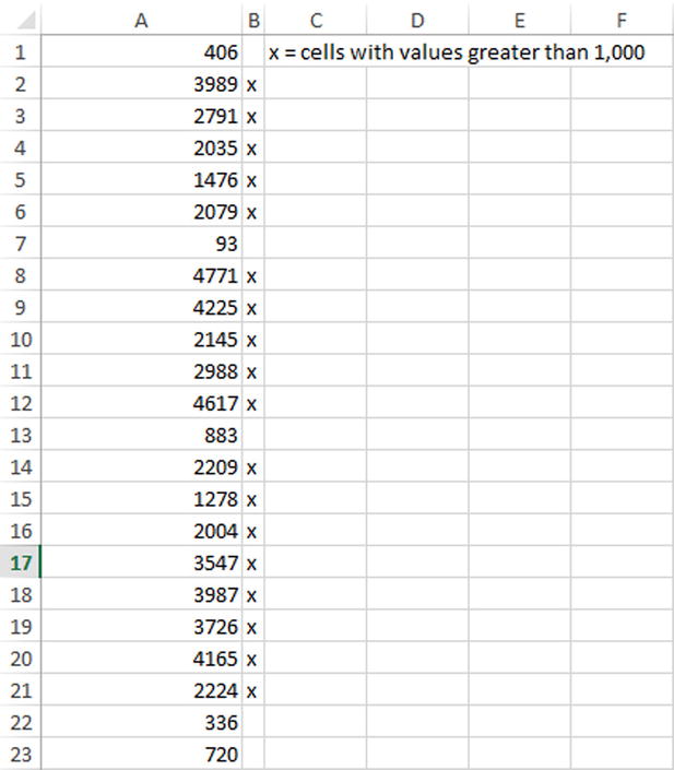
Figure 7-1. An example of where I’m using a signal, in this case an x, to identify values greater than 1,000
You can use the code shown in Listing 7-1.
In particular, notice the code section in bold. Rather than simply setting the value to an x, you’re first testing whether it’s already been set (perhaps from a previous iteration). If it’s already been set, you’re not going to set it again. Remember, every time you change the value of the cell, you’re committing a volatile action. Simply testing whether a property has already been set can help you limit such actions. I’ll go into this in more detail later in the subsection “Testing Properties Before Setting Them.”
In the meantime, you can limit such actions altogether by employing formulas instead. For instance, in the cells next to each value, you can employ a formula to test the values of the numbers. You simply add the formula in cell B1 and drag down. Then every update made to these numbers does not require the code in Listing 7-1 because the formulas will update the signals in real time. This method completely avoids volatile actions to set the signal (Figure 7-2).

Figure 7-2. Using formulas next to each number is a way to bypass using VBA to write an x every time
Finally, you can employ custom formats, which allow you to bypass formulas altogether. For instance, in Figure 7-3, I’ve first set each cell in B1 to be equal to the cells in A1.

Figure 7-3. The first step in applying custom formats to signal which cells are greater than 1,000
You can then highlight the entire range created in column B, right-click, and select Format Cells. Within the Format Cells dialog box that appears (Figure 7-4), you can use the custom formatting code [>1000]"x";"" to set any value that is greater than 1,000 to x and leave all other potential values in the series as a blank string. (I’ll go into using these custom format conditions in later chapters.)

Figure 7-4. Applying a custom format to the cells in the list
Applying this custom format will achieve the same results as the other examples presented. And each example presents its own costs and benefits. The VBA code method is easy to follow and understand. The formula method is faster, but when you have a lot of data and a more complex example of setting a signal (or even a series of signals), the VBA method might prove faster. The custom format method wins on speed over all the other methods (since it requires virtually no calculation to assign from one cell to another), but custom formats aren’t commonly used in this way, and some spreadsheet users without familiarity with the custom format might look at the series of x’s in puzzlement.
What you choose to use in your work must be weighed against these factors. It’s important that you are continuously looking for ways to achieve the same results while committing the fewest volatile actions as possible. This will allow you to perform complex calculations and display complex data without grinding your spreadsheet to a halt.
Adding, Deleting, Filtering, Hiding/Unhiding Rows and Columns
Another volatile action involves making changes to the design of the spreadsheet. Specifically, telling Excel to add, delete, filter, or hide a row will cause a recalculation.
Pivot tables are among the worst offenders in this regard. I break from my colleagues on the use of pivot tables for many of the types of dashboards you’re building here. They seem like an obvious choice for dashboards because of their ability to summarize data. But their drill-down and filtering capabilities result in volatile actions.
Figures 7-5 and 7-6 show how pivot tables cause volatile actions.

Figure 7-5. A pivot table with a collapse row label
In Figure 7-5, you see several collapsed row labels. If you want to drill down, Excel must write that new information to the spreadsheet. Figure 7-6 shows the pivot table expanded.

Figure 7-6. The same pivot table with Human Resources expanded
This innocuous action causes the inevitable recalculation. In fact, you can test this for yourself by placing the following code into the worksheet object code:
Private Sub Worksheet_Calculate()
    MsgBox "Calculation Initiated!"
End Sub
There is one caveat, however, and that’s using pivot tables in conjunction with much of the new capabilities implemented in Excel 2010 and expanded upon in Excel 2013. Pivot tables, when used in conjunction with slicers and other tools, such as power queries, can be rather powerful. However, again, you must gauge the use of this power in the context of unwanted volatile actions. Previous books on dashboards and interactive reports have presented pivot tables as a great feature for dashboards. However, in practice, pivot tables often overwhelm dashboards and become so large and unwieldy that they are a major cause of slowdown. That is why we will hold off on using pivot table capabilities until the final chapters of this book. I want to show you how you can achieve much of the same capabilities with formulas and code while greatly minimizing volatile actions.
Disabling and Then Enabling the Calculation State
In this section, I’ll talk about how changing the calculation state can cause volatile recalculations, negatively affect spreadsheet speed, and create wonky errors.
It’s common practice, much to my dismay, to disable calculation when a spreadsheet has become unwieldy. There are certain instances, especially when you are using Excel to explore a problem, when you must disable calculation but only temporarily (for instance, you receive a spreadsheet with unclean data and the process to clean it requires you to temporarily suspend calculation just to set up formulas to get the data in good condition). Dashboards and reports, however, deal with the presentation of data and not its exploration. Let me say this rather definitively: there is no good reason your dashboards, reports, and applications should ever have to disable calculation.
For the uninitiated, there are two ways you can disable (and subsequently enable) automatic recalculation. You can disable automatic recalculation yourself through Excel’s ribbon by going to the Formulas tab and clicking Calculation Options ![]() Manual (see Figure 7-7).
Manual (see Figure 7-7).

Figure 7-7. Manually setting the calculation state
This method of disabling calculation, that is, manually through the ribbon system, often happens when you must clean data. Again, I’m not against turning off manual calculation temporarily. As well, you can disable automatic recalculation within VBA, using the following code to turn it off:
Application.Calculation = xlCalculationManual
You can use the following code to flip it back on:
Application.Calculation = xlCalculationAutomatic
However, this second form of disabling calculation through VBA is both common and terrible. From a functional standpoint, there’s no difference between changing the calculation state either in the code or manually on the ribbon. However, in practice, when calculation is turned off in the code, it’s often because the programmer is asking too much of Excel (that is to say, they haven’t read this chapter yet).
The problem with turning on manual calculation, especially before doing some complex calculations in VBA that must interface with the spreadsheet, is that things can become screwy quickly. Here’s why: it’s common practice to turn off manual calculation right before some intensive process. However, the programmer will still require some cells to calculate. In these instances, the programmer will select a few active cells and have them calculate the formulas stored therein.
When a cell’s value has changed (remember, this is a volatile action), Excel will mark that cell in its calculation algorithm as becoming “dirty.” The process of recalculating every cell in the calculation chain is what makes it clean again. But if an intensive loop were to error out, there may be a series of cells that are clean having been calculated and still some that are dirty. There’s no way to tell of course which is which. That information is stored internally. If you’ve messed with the calculation state before in this way, you probably know what I’m talking about. Some cells may have correctly calculated values; others not. It’s just not worth the headache.
The long and short of it is this: when you select Manual in the set Calculation Options drop-down list, you lose control of the calculation process, which you should be in control of. If you plan correctly and avoid (or, at least, mitigate the unavoidable) volatile functions and actions, you won’t run into a situation in which manual calculation feels like a viable option. But you might be relying on certain calculations to be performed on your spreadsheet that setting the calculation to manual will prevent from executing. And it’s often forgotten that when you once again set the calculation to automatic, a full recalculation is executed. Full recalculations recalculate everything on the spreadsheet. And if you have complicated formulas, the result might express itself similar to Figure 7-8.
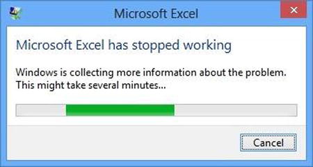
Figure 7-8. Don’t let unruly calculations do this to your spreadsheet
So, I strongly recommend against changing the calculation state. If your spreadsheet is moving slowly, this chapter (and the rest of the book) will contain optimization tips that might help.
![]() Caution Don’t use Application.CalculationState = xlCalculationManual. There’s almost always a better way.
Caution Don’t use Application.CalculationState = xlCalculationManual. There’s almost always a better way.
Understanding Different Formula Speeds
In this section, I’ll discuss how the choice of formula can affect the speed of calculations. This subject is rather vast, and the subsection here won’t do it justice. For an example, you’ll look at how speed differences manifest in the process of data lookups. But for a more lengthy explanation and too see advancements in this area, see the work of Excel MVP Charles Williams and his blog, “Excel and UDF Performance Stuff,” at https://fastexcel.wordpress.com/.
Lookups refer to finding relevant data from different parts of the spreadsheet. Lookups are important to dashboards because they’re used to report results among other capabilities. Common lookup functions include VLOOKUP (naturally), INDEX, and MATCH. The next two subsections discuss advantages and common pitfalls in using VLOOKUP and why INDEX and MATCH sometimes prove to be a better choice.
The most common lookup formula is probably VLOOKUP. One advantage of VLOOKUP is that it’s pretty easy to use and understand. VLOOKUP searches through each possibility in the first column to match the supplied lookup value. In the worst-case scenario, it must look through every element to make a match if the desired value is at the bottom of the list or to discern that it’s not even in the list at all. Therefore, in terms of performance on large lists, many VLOOKUPs can become slow.
And, in many instances, VLOOKUP might be better replaced by using the INDEX function. These instances exist where there is some inherent ordered list structure in the data to be traversed. For example, in the example in Figure 7-9, you can get by without using VLOOKUP. Since the program list is in order and the last character of each item is a number, you could use INDEX to pick out the program in the third row instead of using VLOOKUP to find “Program3.” (See Figure 7-9.)

Figure 7-9. An example of an inherently ordered list
And, assuming the example holds true in the real world (that is, all the programs include some number at the end of their name that identifies where they might fall in a list), you could use that information for the INDEX function. For instance, let’s say “Program3” was input into cell A1; you could then use the function RIGHT(A1,1) to return the first rightmost character in the string. This would return the number 3—the row number you’re interested in. In full, you could then use the function =INDEX(D2:D10, RIGHT(A1,1)) instead of VLOOKUP to reference directly the cell you’re interested in.
Another example is where you have used a list of sequential numbers to encode rows or tables. Take a look at the table in Figure 7-10.

Figure 7-10. A table of planning phases organized by ID
You could use this information to define the per-month cost of a project, like in Figure 7-11.

Figure 7-11. An intermediate table to aid in the process of lookups
This information would could then serve as an index lookup to create the table in Figure 7-12.

Figure 7-12. The final table after using the intermediate table to look up values for each phase
It may be tempting to write “Planning” instead of 1 in Figure 7-12, but you don’t need to do this because INDEX works with an ID number. You can also use VLOOKUP on numbers, but INDEX really is the better option. Remember, be on the lookout for when INDEX might do a better job than VLOOKUP.
The examples here are small. It’s not a big deal for VLOOKUP to traverse a small number of values. But as stated previously, VLOOKUP must go through each item in the list to find a match (hence the traversal). Again, in a worst-case scenario, VLOOKUP must go through each item in the list to find a match. To the extent you can minimize traversal, you should.
However, the real world contains messy data that does not always formulate itself so neatly in the previous two examples. VLOOKUP then is particularly useful when data in a list contains no additional information inherent to each data point about its location in the list. The example shown in Figure 7-9 did contain such information, but names in the next example (Figure 7-13) do not.
And, it’s often forgotten that VLOOKUP can return multiple cells at once. Take the table in Figure 7-13, for example. Here you see representatives on the left side of the table and information about their job performance in the fields thereafter.

Figure 7-13. A table showing representative performance data
Let’s consider the table in Figure 7-13. If you wanted to know Jeremy’s performance but only wanted to return his sales figures and whether these figures beat his target, you might be tempted to create two different lookups, as shown in Figure 7-14.

Figure 7-14. Two different lookups to pull back the different associated fields
But VLOOKUP provides a way around this. You could use an array formula instead that stretches across the two cells. You simply need to fill that column parameter with an array of the columns you’d like to pull back. This is shown in Figure 7-15.

Figure 7-15. Using an array formula to return columns 2 and 4
Notice I’ve used those curly brackets to denote an array formula. Also, notice, that the columns to be returned need not be adjacent to one another. Here, returning multiple items at once provides the immediate advantage of turning two (but it could be several, in your case) lookups into one.
![]() Note Remember array formulas always require you press Ctrl+Shift+Enter to return multiple items across multiple cells.
Note Remember array formulas always require you press Ctrl+Shift+Enter to return multiple items across multiple cells.
There’s actually a pretty interesting argument out there against using VLOOKUP. Charlie Kyd, of ExcelUser.com, has run the numbers, and using a combination of INDEX and MATCH is faster than VLOOKUP in most cases and still slightly faster in its worst case. Instead of VLOOKUP, your formula would look like this:
=INDEX(range, MATCH(row_index_num, lookup_array, 0), column_index_num)
The most obvious advantage to using INDEX/MATCH is that the lookup can go in any direction. Remember how VLOOKUP was used in Figure 7-14? Well, VLOOKUP can pull information that belongs only to the right of the first column. But what if you wanted to search who had sales figures of $21,232? You wouldn’t be able to do this with VLOOKUP, but you can easily do this with INDEX/MATCH. Figure 7-16 shows how to do this.

Figure 7-16. Using INDEX/MATCH to look up information to the left of the lookup column
Spreadsheet errors are a major cause of slowdown for spreadsheets. Think #DIV0! errors are innocuous? Think again! They can contribute to major bottlenecks in your spreadsheet.
Often spreadsheet errors are lurking in parts unknown of your spreadsheet, relics of work you no longer need. You can hunt them down by using Excel’s Go To Special capability. Simply click Find & Select on the Home tab and then select Go To Special. Figure 7-17 shows how to do this.

Figure 7-17. You can find the Go To Special feature under Find & Select on the Home tab
Once you see the Go To Special dialog box (Figure 7-18), select the Formulas option and clear every check box except for the Errors box. This will take you to the errors on your spreadsheet.

Figure 7-18. The Go To Special dialog box
After clicking OK, all spreadsheet errors will be highlighted. What you want to do with those highlighted pieces is largely up to you. If they are an integral to your model, the easiest way to fix them is by placing an IFERROR around the formula. The following code shows the prototype for the IFERROR formula:
IFERROR(value,value_if_error)
The first parameter, value, is where you place the original formula to be evaluated. The second parameter, value_if_error, is where you place what you want the function to return only if an error results in the first parameter. This is a great way to capture error-prone cells in your worksheet.
Alternatively, I’ve found errors like these abound in forgotten and no longer used sections of spreadsheets. Using the Go To Special directive as I’ve done here might especially helpful for finding parts of the spreadsheet that are no longer necessary. Consider deleting them in addition to the #DIV/0! Table 7-1 shows spreadsheet errors to look out for.
Table 7-1. Common Formula Errors
|
Formula Error Name |
Description |
|---|---|
|
#DIV/0! |
This is returned when a zero is supplied as the divisor in a quotient. |
|
#VALUE! |
This is returned when the wrong type is supplied to a formula. For instance, =SUM(1,"2") would return this error. |
|
#REF! |
This is returned when the range referenced no longer exists. For instance, if column A is deleted, then a cell with the formula =A1 would return the #REF! error. |
|
#NAME? |
This is returned when a formula function is misspelled. |
|
#NUM! |
This is returned when you supply numbers into a mathematical function like IRR or NORM.DIST that violate underlying mathematical properties. |
I bring all of this up to demonstrate that formulas can and do slow down spreadsheets. However, you can go too far in making your formulas super speedy, realizing only small gains while making unreadable formulas. Therefore, there will always be some consideration you’ll have to go through when choosing which formulas to use. Ultimately, however, if you build with speed in mind, then taking a few liberties with formulas won’t kill a spreadsheet, but a lot of liberties will.
Code Pitfalls
Of course, formulas are only part of the problem. In this section, I’ll talk about coding pitfalls. It’s worth revisiting here an example that was shown in both Chapters 1 and 5. Specifically, you should attempt to avoid as much iteration as necessary.
You could use the following code that iterates ten times:
For i = 1 To 10

    Sheet1.Range("A" & i).Value = ReturnArray(i)

Next i
or you could use one line of code, as shown here:
Sheet1.Range("A1:A10").Value = ReturnArray
The speed gain here is significant when the examples become nontrivial. In the first iteration example, Excel must write to the screen ten times. Each of these writes is a volatile action that will command a recalculation. On the other hand, the second line of code requires only one write action (and only one recalculation). In other words, the one line in the second example code can complete the same amount of work in one-tenth the time as the first example. Indeed, if the iteration in the first example was for 100 items, the second code line (properly updated to reflect 100 items) would take 1/100th the time to complete as the iteration method.
What should be absolutely key to avoid is the use of copying and pasting via VBA. It’s common for those simply starting out with Excel to record a macro of a copy-and-paste action. Listing 7-2 shows such code I recorded with a macro.
Often, this code is edited and then placed into a loop to re-create the action many times. However, each paste is a volatile action. Moreover, the clipboard—where the information that’s been copied is stored—is not controlled within Excel. It’s not uncommon for it to be cleared out when an intervening process—sometimes a process you’ve instantiated with Excel and sometimes a Windows process—to clear out the clipboard. You can’t rely on the clipboard to store information. For that, as I’ll talk about this book, there are variables and the spreadsheet as a storage device.
Testing Properties Before Setting Them
In this section, I’ll discuss a technique of testing properties before setting them. I first read about this technique in Professional Excel Development. Given that it requires some extra code, it may feel out of place. One would think it less efficient. For instance, let’s say you have some loop that runs through a series of cells and sets specific cells in those series to be bold. Testing whether a cell is already bold before turning it bold would look something like this:
If CurrentCell.Font.Bold <> True then CurrentCell.Font.Bold = True
This setup may look awkward, but it proves to be much faster for certain types of problems. Often you’ll have situations where you must iterate through a series of cells that will already have the changes (such as making a cell bold) applied the last time you ran the code. You’re simply rerunning the code to reflect updates made when data was updated in the list. You don’t need to set a cell to a specific format if that format was already set previously. The action of testing whether a format has been set is actually must faster than changing the format itself. So, by not repeating redundant actions, you can greatly speed up the code.
Let’s see this in a larger example. Let’s say you have a spreadsheet with a series of columns with numerical values in them. Figure 7-19 shows what I’m talking about. You can see this file in action: download Chapter7TotalExample.xlsm.

Figure 7-19. Columns of numerical values with different size columns
This example was inspired by a question I saw proposed on an Excel forum. The poster had a spreadsheet similar to this but with many, many more KPIs. Their goal was to highlight in yellow and make bold the numbers under each Total. As you can see in Figure 7-18, some of the numbers are already highlighted and bold, but not all.
The typical way to solve this problem with VBA is to find the Total cell and then make each cell underneath yellow and bold. Listing 7-3 shows a code example that can do this.
Take a look at the bold code in Listing 7-3. Notice that it sets the cells to yellow and bold every time. But, as Figure 7-19 demonstrates, there may be occasions when these cells are either already bold, yellow, or both. It would make more sense to test each cell first before making the change. Listing 7-4 shows these updates.
Again, this may seem inefficient at first because it involves extra code. However, changing the property of an Excel object, like a cell, is a much more intensive process for Excel. Simply testing common properties before setting them will cut down on repetitious changes that Excel could avoid. Indeed, this idea can be extended beyond cell formats. It applies to all objects in Excel that have properties you can set. For instance, perhaps you are iterating through a series of shapes or through a series of worksheet tabs. The same principles hold.
Bad Names
In the previous chapter, I talked about correct naming conventions for variables. In this section, I’ll extend that concept to file names and worksheet tab names. You may be wondering whether this section even belongs in this chapter or in this book. File names and worksheet tab names are often left to the preferences of the user or to organization policy. In my experience, however, such policies (or, alternatively, such lack of good policies) have led to file names that are incomprehensible to other users and clients. Not only do good names help you understand what’s going on, but in the case of spreadsheet file names, they also help you understand how your work has evolved over time.
Let’s direct our focus to file names first.
Different organizations might have policies directing you to how you should name your files—or perhaps you have preferences you’ve developed over the years that guide how you name files. However you choose to name files, the names should be descriptive and understandable to more than just you. This simple point is often forgotten. Figure 7-20, for example, shows several versions of dashboards. Can you tell which file is the most recent version?

Figure 7-20. A common-looking list of files
The most recent file in this list is SalesDash_O4-03-12 JMG 05-09-2013B.xlsx. Now let’s compare the list in Figure 7-20 to the same files renamed in the list shown in Figure 7-21.

Figure 7-21. Better file names help with organization and file archiving
This may seem trivial, but proper file names will help you keep track of your progress. In the “Proper File Name Style” sidebar, I’ve outlined some common rules to name your files.
PROPER FILE NAME STYLE
What follows are five style rules that should help you have more descriptive file names.
Use Your Words
An ideal Excel file name should be two or three succinct words and contain few numbers. Current operating systems no longer constrain file name character length, so there is no excuse for or cleverness in using shorthand. Capitalize each word as you would a document title.
If your file is an example to someone, it should have the full word “Example,” not “ex,” in its title. If your Excel dashboard is the second version of the “Cost Analysis and Reporting System,” you may abbreviate your file name to “CARS v2.xlsx,” but a VBA Chart Tutorial should never be named “VB ChrtTut.xlsm.”
Always Connect Words with a Space and Nothing Else
The name of your file is not a programming variable or engineering quantity. The words in your file name should not be connected with underscores (_) or dashes (-).
Use Clear Dates, but Don’t Include Dates in Every File Name
Unless your file is a report that comes out on a specific, periodic schedule, there’s likely not a good reason to put today’s date in your file name. If you must put a date in your file, place the date at the beginning, left side of the file name so it appears first. This ensures the date is not cut off when viewed in a file explorer. Dated files are likely to be stored with similar files in the same folder, so cutting off the last bit of each file name on the right is less harmful than cutting off the date.
Numbers Are Preferable to Dates
If you have several iterations of a file, use a numbering system instead of dates. Using dates leads to the horrible practice of adding extra numbers at the end of the file name, for example InventoryList 22 Feb 2001_1.xlsx, InventoryList 22 Feb 2001_2.xlsx, and so on. Moreover, using dates and the former practice will not instantly make clear which is the latest version of your file when viewed in a file directory. However, placing a number at the end of your file name (Inventory List 1.xlsx, Inventory List 2.xlsx) always will make clear the latest (and first) iteration of the file whether sorted by file name, file type, or date modified when viewed in a directory (these files will always be either first or last). Numbers always should appear as the last character on the right.
You can extend this idea to worksheet tab names. You should just be mindful of undescriptive names creeping into your work. Compare Figure 7-22 to Figure 7-23.
![]()
Figure 7-22. A worksheet with terrible tab names
![]()
Figure 7-23. A worksheet with terrific tab names
I don’t have specific guidelines for tab names except to follow the theme presented so far. Use spaces to separate words, use descriptive names as much as possible, and keep others in mind as you work. You never know who else might take up your work after you’ve left. Or, perhaps several weeks, months, or even years later you’ll have to revisit your old work—you’ll thank yourself for using descriptive and commonly understood titles in place of retired acronyms and jargon no longer in vogue.
The Last Word
In this chapter, I discussed many of the pitfalls of development. They come in several forms: calculation, code, and design. The concepts presented are not hard-and-fast rules. Rather, they are principles to keep in mind as you develop. Sometimes you will have to break a rule or toss out convention. But keeping convention in mind is what allows you to know when to break a rule. When you develop with intention, the work you create is far superior.
In the next chapter, you’ll delve more deeply into dashboard layout.