
![]()
An Interactive Gantt Chart Dashboard, Data Details on Demand
In the previous chapter, I went through the visual elements of your Gantt chart dashboard. In this chapter, I’ll go through developing the interactive pop-up that presents details on demand about a specific date in time. Figure 15-1 shows this pop-up for Project 1, Day 2.

Figure 15-1. The details-on-demand pop-up mechanism shows details for a specific project and day
This mechanism was first described in Chapter 5. Officially, the rollover mechanism is a bug in Excel you’re exploiting to create something new. Before I go into how it’s implemented in this dashboard, let’s take a moment to review from a high level how it works. Therefore, this chapter is split up into two parts. First, I’ll discuss the Rollover Method in more detail and demonstrate its utility as a reusable component; next, I’ll show how it can be easily implemented into the Gantt chart.
The Rollover Method
In this section, I’ll review how the Rollover Method works. In the first subsection, I’ll review a simple example of the Rollover Method. In the following subsection, I’ll go into a more advanced example and present a conceptual method for how to implement the method.
A Quick Review of the Rollover Method
As you might recall, the Rollover Method works by breaking one of the tried-and-true rules of Excel: user-defined functions (UDFs) are not allowed to make changes to the spreadsheet. However, an interesting thing happens when you place a UDF in the HYPERLINK function of a cell. The UDF will call the macro. Let’s take a look at an example user-defined function.
Into a module I’ve added the code in Listing 15-1.
Then, on a free worksheet, I’ve added the following function to cell A1: =IFERROR(HYPERLINK(MyRollover("Hello World"),"Hover Over Me"),"Hover Over Me"). This is shown in Figure 15-2.

Figure 15-2. A demonstration of the rollover technique
Notice Figure 15-2 shows the rollover mechanism in action. When my mouse is placed over cell A1, MyRollover is called where "Hello World" is the argument. If you follow the code in Listing 15-1, you see whatever text is supplied will be produced to cell B1. The formula requires IFERROR surround it since it’s essentially a bug. Without that IFERROR, a #VALUE error would appear in cell A1, which wouldn’t look all that good.
A Conceptual Model for Rollover Method Implementation
In this section, I’ll talk about a more conceptual model of how to implement the Rollover Method in your own work. While it’s nice to change a cell’s value, you want to add more interactivity than that. For instance, it might be nice to understand where the rollover took place. Open Chapter15RolloverDemo.xlsm to follow along.
Figure 15-3 shows a 5×5 grid of cells. Cells J2 and J3 are named CurrentColumn and CurrentRow, respectively.

Figure 15-3. A grid of cells where you’ll implement the Rollover Method
In Listing 15-2, I’ve implemented a user-defined function in a new, unused module.
Finally, take a look at the formula I’ve implemented in each cell in Figure 15-3. In cell C3, you can see the Rollover Method formula implemented. Notice the two cell references that make up the arguments of MyRollover. Figure 15-4 shows this formula in the upper-left of the table at row 1 and column 1. These two cell references are set up to always pull the correct row and column coordinates for any location within the table.

Figure 15-4. The row and column references will always be correct no matter where the Rollover Method is in the table because of correct cell references
To ensure the same when you implement this mechanism, start in the upper-left corner of your coordinate grid table. Remember, if you want to capture the column number, the cell address reference to the column should keep the row number absolute and leave the column letter relative; for rows, you would do the opposite: keep the column letter absolute and the row numbers relative. You can see this dynamic implemented in the formulas in Figure 15-3 and 15-4.
So, let’s review what’s happening before moving forward. First, you defined a region of rollovers in a grid layout. Next, you implemented a Rollover Method formula and user-defined function that would capture the location of the cell that triggered the rollover user-defined function. You did this by capturing the row and column indices and sending them to the user-defined function. Within the user-defined function, you tell Excel to write the current location to the spreadsheet. Figure 15-5 shows this mechanism working as intended. The rollover implemented in cell D6 sends the coordinates (row 4, column 2) into the user-defined function, which are then written to the spreadsheet in J3 and J2, respectively.

Figure 15-5. The row and column values sent into the UDF are written to the spreadsheet
Implementing a Hover Table
Now that you know the coordinates of the mouse location vis a vis the cell it’s hovered over, you can add some interactive elements. I like to do this via what I call a hover table. The hover table mirrors the originally defined table grid. However, its purpose is to simply capture the cell currently hovered over. Let’s take a look at an implementation of the hover table in Figure 15-6.

Figure 15-6. An implementation of a hover table. The hover table parallels the rollover table by capturing the relative cell location of the cell being hovered over
Let’s take a look at the formula in Figure 15-6. Recall the AND function is a Boolean logic formula. It returns a true when all conditions specified within the AND function are true. Figure 15-6 shows the formula for the upper-left cell. But if you take a look at the relative references, you can see it is easily dragged right and then down. Because AND is by definition a Boolean function, by default it will return a TRUE and FALSE to signal whether its conditions have been satisfied. You use the shorthand -- to convert TRUE and FALSE to 1 and 0. Technically, you don’t need to do this, but because this dynamic you’ve set up here treats cells as coordinates and the cells are often small, 1s and 0s are easier to read than TRUEs and FALSEs, which often appear as #### anyway given the small cell sizes.
Figure 15-7 should drive the point of all of this home. The mouse is hovering over the cell at (2,2), and the hover table has “lit up” a 1 in the same location.

Figure 15-7. The hover table lights up or “flags” the coordinate location where the rollover has taken place
Implementing Conditional Formatting
With the hover table done, you can easily add all sorts of fun stuff. Let’s say you want a shaded square to follow the mouse. You would do this with conditional formatting. First you would select the rollover region and implement a new conditional formatting rule (Figure 15-8).

Figure 15-8. Conditional formatting can be placed on the rollover region
Next, in the New Formatting Rule dialog box (Figure 15-9), you set Rule Type to “Use a formula to determine which cells to format.” In the “Format values where this formula is true” box, you implement the rule =(C12=1). Notice C12 is the first cell in the upper-left corner of the hover table. Also, notice C12 is a relative reference. For conditional formatting, this means the rule will be test in a pairwise fashion. For instance, cell C3 from the hover table (coordinates (1,1)) will test whether cell C12 is equal to 1. Cell D3 will test whether D12 is equal to one in the hover table, and cell C4 will test against C13. Take a look at Figure 15-9 to make sure you understand this concept.

Figure 15-9. You use a relative reference as the conditional formatting rule
Once you’ve set up the rules, you can click the Format button to specify how you want a cell triggering the rollover to appear. In Figure 15-10, I’ve made a simple change. I’ve set rollover cells to show a red border wherever the mouse hovers in the region of rollovers. Once I’ve set this change, I’ll click OK until I get back to the spreadsheet.

Figure 15-10. The Format Cells dialog box
Figure 15-11 shows this mechanism in its final form.

Figure 15-11. The red hover square follows the mouse location within the grid of rollovers
The red square may seem like a simple implementation given all the work to create it, but there’s actually a lot more available. You’ll go through some even cooler uses of rollovers in the next few pages. But I wanted to present this dynamic to you at an abstract view. This simple implementation shows the basic setup of rollovers that drives the much more complex implementations.
Figure 15-12 shows a conceptual framework to understand everything you’ve done so far. When you abstract it to this level, its implementation makes sense. Using this framework, the rollovers become a reusable component. You can use this coordinate rollover scheme for many different types of problems you want to model. Not every implementation must follow this dynamic exactly, but it serves as a structure starting from which you can adapt and make changes. You’ll be doing just that in the next section.
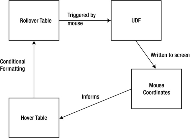
Figure 15-12. A conceptual framework for rollovers
Let’s go back to the Gantt chart. Open file Chapter15GanttChart.xlsm and ensure you’re looking at the top of the spreadsheet. In this section, you’ll investigate the implementation rollover in the Gantt chart. Most of the implementation draws directly from the previous section. I’ll also discuss how to use rollovers to create that details-on-demand pop-up. Gantt chart rollovers
Rollover Implementation
In this section, I’ll show you how the conceptual framework presented in the first section of this chapter has been easily implemented in the Gantt chart.
Let’s start at the top of the Gantt chart. In Figure 15-13, I’ve clicked cell E8 to show you you’re implementing rollovers.

Figure 15-13. Notice the rollover formula follows what you investigated in the first half of this chapter
The row of date headers serves the dual purpose of also letting you know the column index of where the column is located (cell E6). You’ll notice B8 is also being referenced, but it looks empty. However, a column of coordinate numbers actually exists in column B (Figure 15-14). I’ve just set the font color to white to hide them. In Figure 15-14 I’ve temporarily made them the default color so you can see what they look like.

Figure 15-14. The row index numbers are temporarily set to black for the purpose of demonstrating to you they’re there but just hidden
Previously I discussed how information from the back end is presented in the Gantt chart. That information makes up the last two cell references of the hyperlink formula. They appear as E42 in Figure 15-14. For a refresher on how that works, take a look at “The Dashboard Worksheet Tab” in Chapter 13.
For now, let’s scroll down to cell location D62. Notice in Figure 15-15 the Gantt chart implementation follows the same development pattern introduced in the first half of this chapter. Isn’t it great when everything lines up?

Figure 15-15. The Rollover Method implementation follows the same development pattern that was introduced in the first half of this chapter
The Gantt chart then uses the results from the hover table to highlight the selected cell. Figure 15-16 shows the conditional formatting rule applied to the Gantt chart. The beginning of the hover table is cell D62. Notice, again, that D62 is not an absolute reference. So, the conditional formatting rule applied to each cell in the range directly parallels with the cells in the hover table. When a cell in the corresponding hover table equals 1, the conditional formatting rule will highlight the cell on the Gantt chart.

Figure 15-16. Conditional formatting is used to highlight the cell currently hovered over by the mouse
Now scroll to cell E36. Figure 15-16 shows the row and column values of the current cell location. Notice in Figure 15-17 the name of the cell is Dashboard.CurrentRow. This is where the UDF writes the current row location. Likewise, the cell underneath goes by the name Dashboard.CurrentColumn (not shown, but you can trust me). This is where the UDF writes the current column location.

Figure 15-17. The Rollover Method writes the current row and column location to cells Dashboard.CurrentRow and Dashboard.CurrentColumn. This is similar to the implementation from the first half of the chapter
Now that I’ve shown you how the Rollover Method has been implemented in the Gantt chart, let’s take a closer look at the pop-up mechanism. In the following subsections, I’ll go through how to get the information you need for the pop-up, how to design it, and, finally, how to make it follow your mouse.
Getting the Information to Create the Details-on-Demand Pop-up
In this section, I’ll discuss how to create the details-on-demand pop-up. In Figure 15-18 I’ve taken a snapshot of the pop-up.
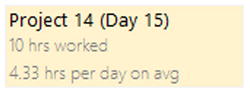
Figure 15-18. A snapshot of the details-on-demand pop-up
Notice you have several pieces of information you need to find out from the data based on the location of the mouse.
- The current project name (Project 14)
- The current day being hovered over
- The current value of hours worked
- The average for the entire day given by the location of the mouse
Luckily, you have the means to find this information by knowing the row and column index of the mouse cell location being hovered over. Figure 15-19 shows the intermediate table starting at C30 and going downward. To help understand what’s going on, I’ve reproduced the formulas for each of these items to the right (the formulas won’t appear in your file). Notice these all simply use the Dashboard.CurrentRow and Dashboard.CurrentColumn formulas defined in cells D36 and D37.

Figure 15-19. The intermediate table with formulas shown
Let’s briefly go through each of them.
- Project name: To find the project name of the currently selected project, you use the current row to find the correct name of the project in the calculations table (Figure 15-20).

Figure 15-20. The project name is found by looking up the current row in the list of project names on the Calculation worksheet tab
- Date: The current date is synonymous with the current column index being hovered over. As shown in Figures 15-19 and 15-20, you just reference Dashboard.CurrentColumn.
- Hours: The hours are simply the raw data values from the data on the Calculation tab at the current row and column index. This is shown in Figure 15-21.

Figure 15-21. The hours are simply found by looking up the hours worked for a given date and project
- Average hours for the given day: Average hours for a given day are found by using the current data (the current column index) and looking up the average hours for a given date on the Calculation worksheet tab (see Figure 15-22).

Figure 15-22. The average hours are found by looking at the average hours calculation row on the Calculation worksheet tab
Now that you have all the information you want to display, you need to design the pop-up.
Designing the Pop-up
If you’ve been following along with your worksheet open, you probably noticed there exists a formatted region in cells AI31:AI33. You can see it all the way over to the right in Figure 15-23. This is where you design the pop-up.

Figure 15-23. The pop-up is designed on the spreadsheet. You can see it in cells AI31:AI34
Let’s take a closer look at the formulas for the pop-up (Figure 15-24). For the first line (cell AI31), I’ve simply set the cell to have a bold format. I’ve used the formula shown in AJ 31 to display the project name and current date highlight. For line AI32, I display the hours worked and add the text “hrs worked.” In cell AI 33, I take the average hours returned for a given data and use the TEXT function to format it so that it displays the values out to the second decimal place only. I add the text “hrs per day on avg” afterward.

Figure 15-24. The pop-up simply references the values from the intermediate table
The background of the pop-up is simply a paint fill, and the border is a soft gray cell border. But you can design yours however you want. The design of the pop-up happens on the spreadsheet, so you are limited only by what Excel allows you to do to the cells.
So, I know what you’re thinking: how do you get this pop-up designed on the spreadsheet to follow your mouse via the Rollover Method? I’ll give you a hint on what’s coming next: say cheese!
Making the Pop-up Follow Your Mouse
In this section, I’ll talk about the last step in creating the details-on-demand pop-up. In the previous sections, I discussed how to grab the information and then how to design the pop-up. In this section, I’ll show you how to create the final piece of the mechanism that will allow the pop-up to follow your mouse.
You’re probably wondering how you get that information designed on the spreadsheet to follow the mouse. Well, ideally you remember the Camera tool from Chapter 5. (I always keep my camera handy!) You’ll use the Camera tool to take a snapshot of the pop-up. Let’s go through what you need to do.
- Select the pop-up area.
- Click the Camera tool.
- Click the spreadsheet to paste the Camera tool shape.
- Get rid of the hideous black border that appears by default (Format Context Ribbon Tab
 Picture Border No Outline).
Figure 15-25 shows how to do this visually.

Figure 15-25. A visual demonstration following the previous steps
Remember the Camera tool provides a live connection to the spreadsheet. So, because the designed pop-up on the spreadsheet updates with new information, the picture created from the Camera tool will update as well.
Once you have a shape for the pop-up, you need to give it a name so you can reference it accurately in the VBA code. The easiest way to change a shape’s name is to select the shape and change its name in the name box next to the formula bar. As you can see in Figure 15-26, I’ve given the new shape pop-up the simple name of Popup.

Figure 15-26. I’ve named the pop-up shape Popup by replacing its default name in the name box next to the formula bar in the upper-left corner of the figure
Next, let’s turn to the rollover-based user-defined function to implement the code that will make the textbox follow the mouse. Take a look at that code in Listing 15-3.
Ideally this should look somewhat familiar to you by now. The row and column variables are passed into the function and then assigned to Dashboard.CurrentRow and Dashboard.CurrentColumn, respectively. I’ve added the additional check If Not [Dashboard.CurrentRow].Value = row and If Not [Dashboard.CurrentColumn].Value = column before the assignment of each so you don’t write redundant information to the screen.
![]() Tip Each screen write is a volatile action. In addition, as your mouse hovers over a cell, the rollover UDF will continuously fire. So, if the values aren’t changing, there’s no reason to continually write the same information and cause recalculation of both volatile functions and nonvolatile functions that might rely on this information.
Tip Each screen write is a volatile action. In addition, as your mouse hovers over a cell, the rollover UDF will continuously fire. So, if the values aren’t changing, there’s no reason to continually write the same information and cause recalculation of both volatile functions and nonvolatile functions that might rely on this information.
Let’s take a look at the second half of the UDF excerpted here:
If [Dashboard.Hoursworked].Value = 0 Then
    Dashboard.Shapes("Popup").Visible = msoFalse
Else
    Dim CurrentRange As Range
    Set CurrentRange = [Dashboard.GanttChartArea].Cells(row, column)
    With Dashboard.Shapes("Popup")
        .Visible = msoTrue
        .Top = CurrentRange.Top.
        .Left = CurrentRange.Offset(0, 1).Left + CurrentRange.Offset(0, 1).Width / 2
    End With
End If
The first condition, If [Dashboard.Hoursworked].Value = 0 Then, tests whether the mouse is hovering over a cell that has information for the given date. Remember there is white space on your Gantt chart where there is no information to report because either a project hasn’t started or one has already ended. Dashboard.Hoursworked is captured on the spreadsheet (Figure 15-27) and reflects how many hours have been reportedly worked. If no hours are available to be reported, that means the given project for the given date has no data to report; therefore, it returns a zero. In instances where there’s nothing to report, you don’t want the pop-up to show. So, you set the pop-up to hidden using the following code: Dashboard.Shapes("Popup").Visible = msoFalse as is shown in the excerpted code.

Figure 15-27. The Intermediate Table showing Dashboard.Hoursworked equals zero
Now that you understand how to build rollover popups, you can use them in your own work. But before you begin implementing them, let’s consider the following tips and concepts. Rollover popups can be complicated and these tips and concepts will help you avoid headaches along the way.
- Use the Selection pane to deal with pop-ups.
Once you’ve prevented the rollovers from executing, the pop-up might still be invisible. Perhaps you moved your mouse over a cell with zero hours worked, which would make the pop-up disappear. To make it reappear, go to the Find & Select drop-down on the Home tab and select Selection Pane (Figure 15-28).

Figure 15-28. You can find the option Selection Pane in the Find & Select drop-down on the Home ribbon tab
In the Selection pane, find your pop-up and click the blank space next to Popup to make the eyeball icon reappear (Figure 15-29). This will signal that the item selected is now visible. You can also make it invisible by clicking the eyeball again.

Figure 15-29. You can toggle the visibility of the pop-up (or any shape, really) by clicking the eyeball icon in the Selection pane
- Remember that you’re exploiting a bug.
If you follow the development patterns presented here, you should be just fine. That is, use the UDF to mostly write to the spreadsheet. Then, use other Excel features to go from there. Don’t use the UDF to generate a new text box from scratch, design and fill it, and so on. This is asking a lot of Excel for a bug. So, keep as much as possible outside of the UDF so that you can ensure it works.
- Save early and often.
That’s just smart.
The Last Word
In this chapter, you accomplished a lot with only a little code. To the extent possible, you used the spreadsheet to aid you in your development. You also used formulas and the Camera tool to ensure you are always dealing with live data. Finally, you saw how the Rollover Method can present you with details on demand. This mechanism represents a reusable component.
You must remember that thinking outside the cell is more than understanding the underlying mechanism. It’s how you can reapply them to different scenarios. As a reusable component, the Rollover Method is extendable to many more situations than presented here. Once you understand its underlying mechanism, you can easily apply it elsewhere.