![]()
Working with Form Controls
When introducing controls, I like to use my own technical definition. Specifically, form controls are the whiz bangs, doodads, whatchamacallits, and thingamajigs that give your spreadsheet enhanced interactivity. You may know them by their street names: check boxes, scroll bars, labels, etc. Figure 16-1 shows a group of controls lounging about in their natural habitat, the Excel spreadsheet.

Figure 16-1. Examples of controls on a spreadsheet
Welcome to the Control Room
Excel contains two types of controls you can use on your spreadsheets. The first are form controls, and they are the subject of this chapter. The second are ActiveX controls, which we won’t deal with in this book. There are significant differences between the two types of controls; however, they’re both located in the same Insert box button, in the Controls group on the Developer tab. One important difference worth noting is that form controls are always on top, ActiveX controls are always on the bottom (see Figure 16-2).

Figure 16-2. The dropdown menu showing form controls and ActiveX controls
Let’s take a moment to discuss why ActiveX won’t make an appearance in this book. In many ways, form controls are leaner, more lightweight versions of their ActiveX counterparts. For example, the ActiveX button can handle several different types of click events. It can test if you double-click or right-click, or it can fire an event the moment your mouse button is pressed down but before it’s released. In theory, the added functionality may feel like a boon of capabilities has been dumped on your lap. In practice, and especially in this author’s experience, rarely does your spreadsheet require that level of advanced functionality. In addition, ActiveX controls carry some baggage to your memory usage and file size; moreover, they can sometimes act unpredictably on a spreadsheet. Figure 16-3 shows the Slider Bar control acting up by appearing unexpectedly in the corner of the screen.

Figure 16-3. A very common ActiveX issue: the Slider ActiveX control appears in both the upper-right side of the sheet and its initial location on the spreadsheet
Form controls, on the other hand, are much more lightweight. However, they are also much more limited in what they can do, at least compared to their ActiveX cousins. And, unlike ActiveX controls, form controls can do a lot without any VBA. In fact, this is one of the reasons I love form controls. Following the ideas presented in Chapter 6, if you don’t need to use VBA, you shouldn’t. Below, I begin with the fundamentals of form controls and present a few examples that will serve as reusable components continuing throughout the book.
Form Control Fundamentals
Think of form controls as simply an extension of the formulas you learned how to use in previous chapters. Those formulas relied strongly on the spreadsheet for the storage and manipulation of values. Figure 16-4 shows an interactive legend that lets the user check “on” and “off” for which series they want to view.

Figure 16-4. An interactive legend using the form control CheckBox
Behind this interactive legend is the form control CheckBox. The CheckBox links to a cell location that either results in a TRUE or FALSE depending on whether the check box is selected or not. (TRUE = selected; FALSE = not selected.) Since TRUE and FALSE are equal to 1 and 0, you can use these response values in a formula to change the data behind the chart. When the check box is deselected, you do some work behind the scenes to change the number the series data to something that won’t appear on the chart (see Figure 16-5).

Figure 16-5. When the check box is deselected, the line disappears from the chart
I’ll talk more about how to do something like this later in the chapter in the “The Dynamic Legend section”.
As you can see from Figure 16-6, there are a total of ten form controls to choose from. Three of those form controls are grayed out. Those controls will always be grayed out for insertion into the spreadsheet. In fact, the only time they are ever available is for Excel 4.0 Macros, an older technology that Microsoft has deprecated in favor of UserForms and ActiveX controls. Officially, Excel 4.0 Macros are no longer supported so I won’t spend any time on them. Tables 16-1 list all the form controls to insert.

Figure 16-6. The Form Controls dropdown showing controls that are available to insert onto the spreadsheet
Table 16-1. Form Control Descriptions
|
Name |
Icon |
Description |
|---|---|---|
|
Button |
|
Button inserts a gray button onto your spreadsheet. You can assign a macro to be executed when the button is clicked. |
|
ComboBox |
|
The ComboBox is similar to the data validation dropdown you can do in a cell. You can supply the ComboBox a list of data from your spreadsheet. The ComboBox will create a dropdown from which to choose a selected item from that list. |
|
|
The CheckBox inserts a box onto your spreadsheet that you can toggle to be checked or unchecked. You can link a CheckBox to a cell to have it display TRUE or FALSE based on whether it’s checked or not. | |
|
Spinner |
|
The Spinner allows you to insert Up and Down paddles on your spreadsheet. You can link the Spinner to a cell such that when you press up, the cell value increases, and when you press down, the cell value decreases. |
|
|
A ListBox is similar to a ComboBox. However, instead of a dropdown, the ListBox shows a larger list of items that users can scroll through. | |
|
Option Button |
|
The Option Button is similar to the CheckBox. However, groups of Option Buttons are mutually exclusive. That means only one Option Button can be selected at a time, while no such constraints exist on Checkboxes. Similar to Checkboxes, you can link Option Buttons directly to a cell. |
|
GroupBox |
|
A GroupBox has no real interactivity but can surround other controls to create delineation and flow. |
|
Label |
|
A Label is a simple textbox that can be placed anywhere on a sheet. Labels are a bit limited compared to Excel’s native text boxes. |
|
Scroll Bar |
|
The Scroll Bar is similar to the Spinner except the Scroll Bar has an area in the middle in which you can drag the value up or down. But similar to the Spinner, you can link the Scroll Bar to a cell and use the up and down (and drag) paddles to change the cell’s value. |
Next, we’re going to go through my favorite controls. I call them my favorite because of the entire bunch, I believe they’re the most useful. After we go through my favorites, we’ll go through my least favorites—the ones I believe you should avoid in favor of better alternatives available.
The ComboBox Control
The ComboBox control is a useful mechanism that essentially mimics the behavior of a data validation dropdown list. But there is a difference between the two that is worth noting. Figure 16-7 shows a data validation both when a selection is being made (that is, the cell is active) and when no selection is being made.

Figure 16-7. On the left, the validation list dropdown is expanded. On the right, the cell has been deselected
Now compare the aesthetics of the data validation dropdown in Figure 16-7 to the form control ComboBox list in Figure 16-8.

Figure 16-8. On the left, the form control dropdown is expanded. On the right, the form control has been deseltected
Notice the different aesthetics between the two “dropdown” lists. Generally, validation lists are better when you have a column of cells and each cell contains a dropdown, since the dropdown arrow won’t appear in every cell, making for a clear appearance.
To view any control’s properties, select the control and press the Properties button in the Controls group on the Developer tab shown in Figure 16-9—or, right-click a control, select Format Control, and select the Control tab.

Figure 16-9. The Properties Button in the Controls group on the Developer tab
Figure 16-10 shows the Format Control dialog box for the ComboBox control. In this dialog box, you can change various aspects of the form control from the Control tab.

Figure 16-10. The Format Control properties dialog box
Note that you have two fields you can connect to the spreadsheet. The Input Range field allows you to select a desired range to fill the dropdown. The Cell link field allows you to specify a cell to display the index of the selected item.
The ListBox Control
The ListBox control is similar to the ComboBox control in that it also uses the Input range and Cell link fields. However, I believe you can better employ several mechanisms incorporated in the ListBox control, including creating a scrollable list (see Figure 16-11). So I personally don’t prefer using these fields with the ListBox control.

Figure 16-11. The ListBox control contains a scrollable list of elements pulled from the spreadsheet
One reason I prefer the ListBox control to the ComboBox is because I want to be able to see the data all at once. Moreover, as you’ll see when you use the ComboBox, you can make the size of the control however large you want. But no matter how big that dropdown arrow becomes, the control’s font and selection list underneath will always stay the same. Figure 16-12 shows a particular egregious example. Rather than fooling the viewer with these strange aesthetics, you’re better off sticking to ListBox.

Figure 16-12. The combo box is sized much larger than it ever should be
The Scroll Bar Control
The Scroll Bar is amazing and probably my favorite form control. It’s simple but powerful. The basic idea is that you can link the scroll bar’s value to any available cell on a spreadsheet. I’ve done just this in Figure 16-13. As the scroll paddle (that’s the gray bar between the upper and lower paddles) increases, so does the value in C2. Similarly, as it decreases, the value in C2 decreases.

Figure 16-13. A form control Scroll Bar linked to the cell C2
The form control scroll bar contains some other great properties, as shown in Figure 16-14.

Figure 16-14. The Format Control dialog box for the Scroll Bar
Note that the Cell link field refers to same location in the formula bar in Figure 16-13. In Figure 16-14, you can see that the form control Scroll Bar comes with many more field properties than the ComboBox and ListBox controls. You can use the Minimum Value and Maximum Value fields to set the upper and lower bounds of the scroll bar. Indeed, you’ll be doing just that in later chapters of this book. You can also use the Incremental Change field to set how much the value increases or decreases when you press the scroll bar’s paddle. Finally, the Page change field refers to how much of an increase or decrease occurs when you click into the scroll bar itself and not on a upper or lower paddle.
Note that only one of the text fields in the Format Control dialog box (see Figure 16-14) can directly tie to a cell–the Cell link. The other fields shown in Figure 16-14 must be set either manually by a human (through the Format Control dialog box) or programmatically with code. Listing 16-1 shows how to change the scroll bar’s Min and Max fields through code.
Notice if you use the shape object on a form control, the only way you can change properties of a form control is through the ControlFormat object. Alternatively, you can also use the shorthand naming syntax shown in Listing 16-2.
Often, I’ll use the latter method as it is more easily read and intuitively understood. However, you’ll notice when you type the As portion of creating your form control object, Scroll Bar won’t appear on the list. This can become confusing as usually figuring out the correct object requires guessing at the name (e.g. typing “label,” ”checkbox,” and “scroll bar” to see if they take). So I present both options for you to decide. Throughout the book, I’ll prefer the one that to me appears easier to read in context.
The Spinner Control
The Spinner control is fairly similar to the form control Scroll Bar sans the draggable paddle and scroll region between the paddles (see Figure 16-15).

Figure 16-15. An example Spinner control on a spreadsheet
The Spinner control is a useful replacement for a scroll bar in a pinch. However, while the scroll bar can appear both horizontally and vertically on a sheet (see Figure 16-1), the spinner can only appear vertically, as shown in Figure 16-15. You can of course make the spinner larger (and wider, if you’d like), but those up and down paddles will always point in the same direction.
The CheckBox Control
The CheckBox control appears in the first example and it’s incredibly versatile. Like the Scroll Bar, the CheckBox control links to cell whose value you can use. Unlike the Scroll Bar, the CheckBox can only take on one of three values (see Figure 16-16). The first two values you should know by heart: TRUE and FALSE. Respectively, they generate a Checked or Unchecked value in the CheckBox.

Figure 16-16. A demonstration of the three states possible with a CheckBox
However, check boxes can also take on a fuzzy-gray status called a “mixed” state. The mixed state cannot be set directly by toggling a CheckBox, at least not without some VBA. You can set the mixed state manually by using the =NA() formula in the CheckBox’s cell link or by going into its properties dialog box and selecting the Mixed option (see Figure 16-17). You won’t use the mixed state in this book, so for now let’s focus on the TRUE and FALSE dynamic of the CheckBox.

Figure 16-17. The Format Control dialog box for a CheckBox
The Least Favorites: Button, Label, Option Button, and GroupBox Controls
Four controls are left:
- Button
- Label
- Option Button
- GroupBox
In this section I’ll provide a little information on why I don’t care much for these form controls.
The Button Control
I don’t believe you should use the Button control because there are better alternatives. Let’s start by taking a look at the Button control in Figure 16-18. There’s not much you can do with the dated grayish aesthetic.
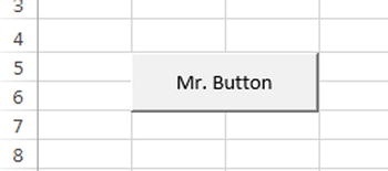
Figure 16-18. A form control Button
An alternative I would suggest is to use an autoshape text box instead. You can still add interactivity to the shape the same way you would with a form control Button by assigning a macro to the shape. The text box will give you much more flexibility in terms of changing its look. In addition, there is no inherent advantage to using the form control Button that is lost when going with an Excel shape.
The Label Control
The Label control is also similarly restrictive. The font size, style, and color of a label cannot be edited directly. Notice in Figure 16-19 that the format buttons have been disabled when the label is selected.

Figure 16-19. A Label control placed on a spreadsheet
As a matter of fact, the only way to change a label’s style is to link it to a cell with the font styles already set. Take a look at Figure 16-20 to see what I mean. In cell A2, I wrote some text and then set the font color and style in the cell itself. After that, I linked the label directly to the cell. In fact, this is a workaround I discovered accidently; officially, labels aren’t supposed to let you change their style. But in any event, a textbox shape does all of this without the hassle.

Figure 16-20. Even bright and wonderful labels can’t overcome certain limitations
The Option Button Control
Option Button controls are similar to check boxes except that they allow for only one selection. In general, I find they are more trouble than they are worth. ComboBox form controls do essentially the same thing as Option Buttons and take up less screen real estate (see Figure 16-21). For situations where I would like the user to toggle between different states, I like to use text boxes instead (see Figure 16-22). The effect is much cleaner and more visually appealing.

Figure 16-21. Option butttons laid out and linked to cell C2

Figure 16-22. My prefered method for toggling between options
Figure 16-22 simply shows a group of textboxes with some extra desired formatting. When a user clicks on a textbox, a macro is called to color the textbox a reddish color and the rest a greenish color.
The GroupBox Control
Finally, form GroupBoxes, the last control left undiscussed, are not really useful for anything except grouping components together. They exist purely for aesthetic value. They’re not ugly by any stretch, but I’d rather use cell formatting to create a border, especially because it delivers far more options. With the form control GroupBox you only get two options: 3D border or no 3D border. For the sake of an example, Figure 16-23 shows a GroupBox form control over the buttons from Figure 16-22.

Figure 16-23. The group box surrounds buttons with the group box’s border
Now that you know all the form controls, you’ll put the useful ones to good use in a few examples, starting with the Scroll Bar.
Scrollable tables are a great form of Excel form controls. They’re easy to implement and often require no VBA, assuming what you want to display isn’t complicated (and usually it isn’t). At the heart of these tables is the venerable scroll bar. Using the INDEX function and the scroll bar you can create a scrollable region from a larger table of values.
In this example, you will create a scrollable table that pulls data from a larger spreadsheet. The scrollable table will allow you to scroll through a small subset of the data a time. Figure 16-24 shows what the final product will look like. Take a look at Chapter16ScrollableTable.xlsx to grab the data and follow along.

Figure 16-24. The final product of your scrollable table
- To start, insert a new scroll bar into the empty spreadsheet tab in the example file. After that, you must assign a scroll bar to a cell that will hold it. In this example, assign it to A4. This is shown in Figure 16-25.

Figure 16-25. Assiging the scroll bar to a cell value
- When creating a scrollable table, you’ll have to decide its dimensions. In Figure 16-24, you can see ten items at a time. You’ll need to set up a series of dynamic indices, so in A4, write the formula A3 + 1 and drag down. Figure 16-26 shows this result and the formulas.
 Tip To help size the scroll bar, use the Snap to Grid feature. Choose a column where you want to house the scroll bar and size the column to the width you’d like the scroll bar to be. Next, after you insert the scroll bar, go to the Format tab and select Snap to Grid from the Align dropdown in the Arrange group. Now resize the scroll bar; you’ll see it easily fits to the column.
Figure 16-26. This dynamic will increase all the numbers in the list as changes to the scroll bar are made
If you try the scroll bar now, you’ll see the dynamic indices increase and decrease with each change in the scroll bar.
- The backend data for this exercise is on the Data tab. The series of years is named TornadoData.Year, the series of tornado totals is named TornadoData.Totals, and the data range is named TornadoData.DataRegion. By naming these regions you can more easily access them with the INDEX function.
Specifically, you can pull the first row of the data region by using the formula INDEX(TornadoData.DataRegion, $A4, ). By leaving that last parameter blank, you can drag the formula across to the desired range and then press Ctrl+Shift+Enter (see Figure 16-27). The last parameter, which takes a column index argument, isn’t necessary in this case. By telling Excel that you are using an array formula, Excel knows that the first cell in the region returns the first column index, the second returns the second column index, and so forth. However, for this to work, you must leave that final parameter blank. INDEX(TornadoData.DataRegion, $A4, ) is not the same as INDEX(TornadoData.DataRegion, $A4).

Figure 16-27. The result of using the Array formula to pull back data
- Once you have the first row, you can simply drag down to fill the entire region, as shown in Figure 16-28.

Figure 16-28. Dragging the array formula down the entire table
- You’ll also need to do the same for the Year column. You need to pull the corresponding cell for the given year from the backend data. Here, you’ll use the formula INDEX(TornadoData.Year, A4) (see Figure 16-29) and then drag down.

Figure 16-29. Use INDEX to retrieve the total tornados for a given year
- Finally, you’ll want to add more information to the table. This example includes the averages for each month over the entire year range by leaving the row index parameter of the INDEX function blank and using a static reference for the column index. This mechanism is similar to what you did above except you are pulling the entire column instead of the entire row. In addition, you are not interested in return each cell in the column; instead, you supply the entire column to an AVERAGE function to get the average for that year (see Figure 16-30).
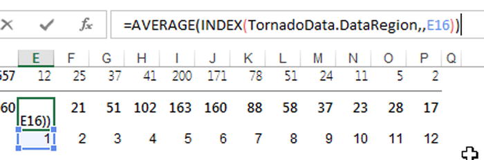
Figure 16-30. Use the AVERAGE and INDEX functions to report the average tornados for each month
- So that the dynamic indices on the left and the static reference on the bottom do not appear in the table, change those cells to a white font, which blends in with the white background.
- Finally, set the Minimum Value and Maximum Value fields of the scroll bar (see Figure 16-31).
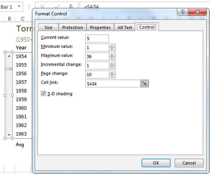
Figure 16-31. The Format Control dialog box
The minimum, of course, is 1. The maximum is 36. Why 36? Well, the entire year range is made up of 45 years. That’s the last year in the set, 1994, minus the beginning year, 1950. (Remember, you’re including 1950 in the set so it comes out to 45 years and not 44.) You show ten years in your table, and you effectively do this by adding nine years to the initial value given by the scrollbar (see Figure 16-32). So the maximum is 45 years minus 9 years, which is 36.
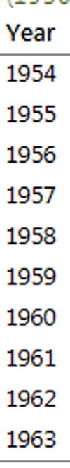
Figure 16-32. Notice that 1963 equals 1954 plus 9
Figure 16-33 shows the final table.

Figure 16-33. The final table
Highlighting Data Points on Charts
You can also use form control scrollbars to highlight a point on a chart. Figure 16-34 shows a time series of the yearly totals of tornados. Below the chart is a scroll bar that moves the black selector point left and right. As the point changes, the label changes with it.

Figure 16-34. You can highlight data points on the chart using a form control Scroll Bar
The setup for this problem is somewhat similar to the last. You can follow along in the example file Chapter16DataPoint.xlsx.
First, you start with a scroll bar. This time, however, you draw it horizontally instead of vertically. Again, for precision, it’s a good idea to use the Snap to Grid feature. Above, you’ll see that columns that border the chart, B and C, are a bit smaller than the rest. I sized these columns about the size of the scroll bar’s paddles. That way, the paddle in the scroll area lines up nicely with the selector on the chart. In addition, I was able to nicely align the plot and chart area again using the handy Snap to Grid feature.
The scroll bar is linked to a value on the side of the Excel spreadsheet. The name of the cell is Scrollbar.Value (gee, how creative…). Using the scroll bar’s value, you pull the X and Y values using the scroll bar as an index (see Figure 16-35).

Figure 16-35. As the scroll bar changes, the X and Y values also change
Now, this is where the magic happens. You’re using a simple scatterplot chart for your timeseries display. Because of this, you don’t have to add a huge series to your chart to show the selector. You only need to add the coordinates defined in Figure 16-36. In your chart, you have a series simply named selector that points to the coordinates off to the side. Remember, those coordinates are traced to the value given by the scroll bar. So, as the scroll bar changes, the coordinates update with each change. That’s how I came up with the nifty effect.

Figure 16-36. The Edit Series dialog box
The other series on the chart is simply the totals from your data worksheet tab (see Figure 16-37).

Figure 16-37. The totals from the tornado data
But wait! This mechanism isn’t complete without grabbing information about the current year. So, let’s add a small chart on the side that displays information for each month of the given year (see Figure 16-38).

Figure 16-38. An additional chart displays information for each month of the selected year
This mechanism is not different from when you looked up rows in the table before. The difference now is that you want to flip that row into a column. So you’ll wrap it in the TRANSPOSE function as shown in Figure 16-39. Once you’ve dragged that function down, you can press Ctrl+Shift+Enter because you’re directing Excel to return a range.
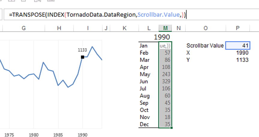
Figure 16-39. The information table relies on the scroll bar’s value to pull monthly tornado data for a selected year
The Dynamic Legend
To make a dynamic legend, you use the CheckBox form control for a series in the chart. In this case, however, you won’t use the legend Excel provides for you as a chart element. Instead, you’ll create your own from scratch! Add three check boxes (clear out the default labels). In addition, write a “minus” sign and add the label next to it, both colored manually. You can see this for yourself by looking at Chapter16DynamicLegend.xlsx with the downloads for this chapter.
Figure 16-40 shows that the legend is simply a cell.

Figure 16-40. The legends here are simply cells
Here’s how this mechanism works: there are essentially two tables that hold the data presented in this graph. The first table is simply static; you can think of it as a type of database. The second table is an intermediary between the database and chart. You can think of the chart as being the presentation layer. The dynamic is laid out in Figure 16-41.

Figure 16-41. The mechanism of a dynamic legend
Let’s take a closer look at the intermediate table. The first column of the table holds the linked cells of the three check boxes (see Figure 16-42).

Figure 16-42. A closer look at the intermediate table
The next column tests whether the link has returned a TRUE or FALSE. If it returns a TRUE, Excel returns a 1; if it’s a FALSE, Excel returns an NA() (see Figure 16-43).

Figure 16-43. If a CheckBox is deselected, you want to return an N/A error
The cool thing about using NA() is that it returns an #N/A error, which Excel won’t plot. In addition to that, anytime you multiply something by an #N/A, it also becomes an #N/A. And that’s exactly what you take advantage of in your dynamic legend. The values in the intermediate table are the product of the result of the IF function multiplied by the original values. Figure 16-44 demonstrates this mechanism.

Figure 16-44. The dynamic legend works by turning the values in a series into an #N/A error and thus removing it from the chart
WAIT…WHY AM I USING IF()? I THOUGHT YOU SAID I SHOULDN’T USE IT?
This is a case where you couldn’t get away from using IF. As you are likely familiar with by now, the CheckBox’s value could be one or zero. Ostensibly, this response would have been perfect as the multiplier. For example, you could have simply written a formula like this:
=(checkbox_response) * original_series_value – NOT(checkbox_response)
You wouldn’t require an IF in this case. If the CheckBox response is TRUE, the original series value is returned (or just multiplied by 1). If it’s FALSE, the original series value becomes a zero and NOT(FALSE) returns a 1; thus, the entire formula of =0-1 results in a -1, which is a point outside the viewing scale of the chart (the chart goes from 0 to 15,000).
Here’s the issue: the dynamic described above works perfectly in Excel 2010, but it does not work as reliably in Excel 2013, at least not as of this writing. You can test for this bug on your own if you are using Excel 2013. Create a new line chart with a series of -1 and set the axis range from 0.0 to 10.0. Chances are, you won’t see the line. Now, change the axis from 0.0 to 20,000. The line will reappear.
But like I said, you shouldn’t necessarily never use IF; rather, you should exercise discretion. In the example, you only use one IF per CheckBox and the rest of the series relies on that IF. This is the best way to do it. You could have alternatively made each datapoint in the intermediate table also be a test against the response of the CheckBox. That would have employed far too many IF statements than necessary.
The Last Word
In this chapter, you learned how truly awesome form controls are. I discussed reusability briefly in Chapter 10, and form controls are an integral part of the reusable components you find on spreadsheets. They’re flexible, don’t often require much code, and can be moved and placed rather easily. As you can probably guess, you’ll return to form controls several times through the rest of the book.