1.1 Basic Statistics

Some of my earliest work using data mining and predictive analytics on crime and criminals employed the use of relatively advanced statistical techniques that yielded very complex models. While the results were analytically sound, and even of interest to a very small group of similarly inclined criminal justice and forensic scientists, the outcomes were so complicated and arcane that they had very little utility to those who needed them most, particularly those on the job in the public safety arena. Ultimately, these results really contributed nothing in a larger sense because they could not be translated into the operational environment. My sworn colleagues in the law enforcement world would smile patiently, nodding their heads as if my information held some meaning for them, and then politely ask me what it really meant in terms of catching bad guys and getting the job done. I rarely had an answer. Clearly, advanced statistics was not the way to go.

Data mining, on the other hand, is a highly intuitive, visual process that builds on an accumulated knowledge of the subject matter, something also known as domain expertise. While training in statistics generally is not a prerequisite for data mining, understanding a few basic principles is important. To be sure, it is well beyond the scope of this book to cover statistics with anything more than a cursory overview; however, a few simple “rules of the road” are important to ensure methodologically sound analyses and the avoidance of costly errors in logic that could significantly confound or compromise analysis and interpretation of the results. Outlined below are some simple statistical terms and concepts that are relevant to data mining and analysis, as well as a few common pitfalls and errors in logic that a crime analyst might encounter. These are by no means all inclusive, but they should get analysts thinking and adjusting the way that they analyze and interpret data in their specific professional domain.

1.2 Inferential versus Descriptive Statistics and Data Mining

Descriptive statistics, as the name implies, is the process of categorizing and describing the information. Inferential statistics, on the other hand, includes the process of analyzing a sample of data and using it to draw inferences about the population from which it was drawn. With inferential statistics, we can test hypotheses and begin to explore causal relationships within data and information. In data mining, we are looking for useful relationships in the information or models, particularly those that can be used to anticipate or predict future events. Therefore, data mining more closely resembles descriptive statistics.

It was not that long ago that the process of exploring and describing data, descriptive statistics, was seen as the necessary though unglamorous prerequisite to the more important and exciting process of inferential statistics and hypothesis testing. In many ways, though, the creative exploration of data and information associated with descriptive statistical analysis is the essence of data mining, a process that, in skilled hands, can open new horizons in data and our understanding of the world.

1.3 Population versus Samples

It would be wonderful if we could know everything about everything and everybody, and have complete access to all of the data that we might need to answer a particular question about crime and criminals. If we had access to every criminal, both apprehended and actively offending, we would have access to the entire population of criminals and be able to use population-based statistics. Similarly, if we had access to all of the information of interest, such as every crime in a particular series, this also would resemble a population because it would be all inclusive. Obviously, this is not possible, particularly given the nature of the subject and the questions. It is a common joke that everything that we know about crime and criminals is based on the unsuccessful ones, those that got caught. Most criminal justice research is based on correctional populations, or offenders that have some sort of relationship with the criminal justice system. Research on the so-called “hidden” populations can be extremely difficult, even dangerous in some cases, as these hidden populations frequently include criminals who are still criminally active. Moreover, any time that we extend beyond official documents and records, we step into a gray zone of potentially unreliable information.

Similarly, we have the disadvantage of relying almost exclusively on official records or self-report information from individuals who are not very reliable in the first place. Consequently, we frequently have access to a very limited amount of the total offense history of a particular offender, because generally only a relatively small fraction of criminal behavior is ever identified, documented, and adjudicated. Criminal justice researchers often are limited in this area because offender interviews regarding nonadjudicated criminal activity approach the “third rail” in criminal justice research. For example, criminal justice researchers must obey existing laws requiring the reporting of known or suspected child abuse. Similarly, researchers should consider the ethical issues associated with uncovering or gaining knowledge of unreported, ongoing, or planned criminal activity. Because this information can cause potential harm to the offender due to legal reporting requirements and ethical considerations, research involving the deliberate collection of unreported crime frequently is prohibited when reviewed by institutional review boards and others concerned about the rights of human research subjects. Similar to drug side effects, there are those crimes and behaviors that we know about and those that we do not. Also like drug side effects, it is generally true that the ones that we do not know about will come up and strike us eventually.

What we are left with, then, is a sample of information. In other words, almost everything that we know about crime and criminals is based on a relatively small amount of information gathered from only a fraction of all criminals—generally the unsuccessful ones. Similarly, almost everything that we work with in the operational environment also is a sample, because it is exceedingly rare that we can identify every single crime in a series or every piece of evidence. In many ways, it is like working with a less than perfect puzzle. We frequently are missing pieces, and it is not unusual to encounter a few additional pieces that do not even belong and try to incorporate them. Whether this is by chance, accident, or intentional misdirection on the part of the criminal, it can significantly skew our vision of the big picture.

We can think of samples as random or nonrandom in their composition. In a random sample, individuals or information are compiled in the sample based exclusively on chance. In other words, the likelihood that a particular individual or event will be included in the sample is similar to throwing the dice. In a nonrandom sample, some other factor plays a significant role in group composition. For example, in studies on correctional samples, even if every relevant inmate were included, it still would comprise only a sample of that particular type of criminal behavior because there would be a group of offenders still active in the community. It also would be a nonrandom sample because only those criminals who had been caught, generally the unsuccessful ones, would be included in the sample. Despite what incarcerated criminals might like to believe, it generally is not up to chance that they are in a confined setting. Frequently, it was some error on their part that allowed them to be caught and incarcerated. This can have significant implications for the analytical outcomes and generalizability of the findings.

In some cases, identification and analysis of a sample of behavior can help to illuminate a larger array of activity. For example, much of what we know about surveillance activity is based on suspicious situation reports. In many cases, however, those incidents that arouse suspicion and are reported comprise only a very small fraction of the entire pattern of surveillance activity, particularly with operators highly skilled in the tradecraft of covert surveillance. In some cases, nothing is noted until after some horrific incident, and only in retrospect are the behaviors identified and linked. Clearly, this retrospective identification, characterization, and analysis is a less than efficient way of doing business and underscores the importance of using information to determine and guide surveillance detection efforts. By characterizing and modeling suspicious behavior, common trends and patterns can be identified and used to guide future surveillance detection activities. Ultimately, this nonrandom sample of suspicious situation reports can open the door to inclusion of a greater array of behavior that more closely approximates the entire sample or population of surveillance activity.

These issues will be discussed in Chapters 5 and 14; however, it always is critical to be aware of the potential bias and shortcomings of a particular data set at every step of the analytical process to ensure that the findings and outcomes are evaluated with the appropriate level of caution and skepticism.

1.4 Modeling

Throughout the data mining and modeling process, there is a fair amount of user discretion. There are some guidelines and suggestions; however, there are very few absolutes. As with data and information, some concepts in modeling are important to understand, particularly when making choices regarding accuracy, generalizability, and the nature of acceptable errors. The analyst’s domain expertise, or knowledge of crime and criminals, however, is absolutely essential to making smart choices in this process.

1.5 Errors

No model is perfect. In fact, any model even advertised as approaching perfection should be viewed with significant skepticism. It really is true with predictive analytics and modeling that if it looks too good to be true it probably is; there is almost certainly something very wrong with the sample, the analysis, or both. Errors can come from many areas; however, the following are a few common pitfalls.

Magnified or Obscured Effects

Uneven distributions also can create errors in the interpretation of link analysis results, which is discussed in Chapter 3. Briefly, link analysis can be a great way to show relationships between individuals, entities, events, or almost any variable that could be considered in crime and intelligence analysis. Some of the new software tools are particularly valuable, in that actual photos of individuals or elements of interest can be inserted directly into the chart, which results in visually powerful depictions of organizational charts, associations, or events. Beyond just demonstrating an association, however, link analysis frequently is employed in an effort to highlight the relative strength of relationships. For example, if Bob calls Joe 15 times, but Joe calls Paul 52 times, we might assume that the relationship between Joe and Paul is stronger than the relationship between Joe and Bob based on the relative difference in the amount of contact between and among these individuals (Figure 1-1).

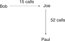
Figure 1-1 Link charts can not only depict relationships between individuals or events, but also relative strength of the relationship based on relative differences in the amount of contact.

These programs often allow the user to establish thresholds for link strength; however, this can provide a false sense of security. For example, in Figure 1-2, it appears that Paul has a stronger relationship with Pete, as compared to his relationship with Joe, based on the relative levels of contact. Bob, on the other hand, appears to have relatively similar relationships with both Joe and Pete, based on relatively equal levels of contact, as depicted in the link chart. Reviewing the related association matrix, however, indicates that this might not be true (Figure 1-3). The actual numbers of contacts indicates that both Paul and Bob had contact with Pete almost twice as much as they did with Joe. The relationship is skewed somewhat in the link analysis chart (Figure 1-1) because the relative levels of activity associated with Bob were much higher than those associated with Paul. As a result, the settings used in the link analysis skewed the visual representation of the relative strength of the relationships noted. For example, in this particular situation, it might be that weak links include 10 associations or less, while strong links require 20 associations or more. Unfortunately, unequal distributions can skew the relative importance of certain associations. In this example, both Paul and Bob had similar ratios of contact with Pete and Joe, a 2:1 relationship, but this difference was magnified in Paul because he was associated with a lower overall frequency of contact. This allowed the difference in his contact with Pete and Joe to be revealed. On the other hand, the same relative difference in the number of contacts Pete and Joe had with Bob was obscured due to the larger number of contacts overall.

Figure 1-2 Examination of this link chart suggests that Paul has a stronger relationship with Pete compared to his relationship with Joe, while Bob appears to have relatively similar relationships with both Joe and Pete, based on relatively equal levels of contact. These apparent differences in the relationships are based on differences in the strength of the association illustrated by relative differences in the lines in the link chart.

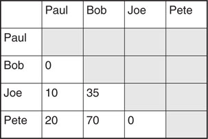
Figure 1-3 This simple association matrix depicts the number of contacts between a group of individuals, and highlights the errors in the associated link chart depicted in Figure 1-2.

Signal-to-noise issues like this can be particularly tricky for at least two reasons. First, they can magnify differences in less-frequent events. Because it takes less to show a difference, it is relatively easy to cross the arbitrary thresholds established either by the user or preset in the software. Second, they can obscure differences in the events associated with greater frequencies. This is particularly true when simultaneously comparing relationships that are associated with very different levels of activity. Again, if the thresholds are not set thoughtfully with an understanding of relative frequencies, some associations can be magnified while other relationships can be obscured. There are a variety of mechanisms available to address this potential confound, including the use of percentages or ratios, which are discussed in Chapter 5; however, the key to addressing this issue generally is awareness and caution when interpreting these types of results.

1.6 Overfitting the Model

Remember the caution: If it looks too good to be true, it probably is too good to be true. This can occur when creating models. One common pitfall is to keep tinkering with a model to the point that it is almost too accurate. Then when it is tested on an independent sample, something that is critical to creating meaningful predictive models, it falls apart. While this might seem impossible, a model that has been fitted too closely to a particular sample can lose its value of representing the population. Consider repeatedly adjusting and altering a suit of clothes for a particular individual. The tailor might hem the pants, take in the waist, and let out the shoulders to ensure that it fits that particular individual perfectly. After the alterations have been completed, the suit fits its owner like a second skin. It is unlikely that this suit will fit another individual anywhere near as well as it fits its current owner, however, because it was tailored specifically for a particular individual. Even though it is still the same size, it is now very different as a result of all of the alterations.

Statistical modeling can be similar. We might start out with a sample and a relatively good predictive model. The more that we try fit the model to that specific sample, though, the more we risk creating a model that has started to conform to and accommodate the subtle idiosyncrasies and unique features of that particular sample. The model might be highly accurate with that particular sample, but it has lost its value of predicting for similar samples or representing the characteristics of the population. It has been tailored to fit perfectly one particular sample with all of its flaws, outliers, and other unique characteristics. This can be referred to as “overfitting” a model. It is not only a common but also a tempting pitfall in model construction. After all, who would not love to create THE model of crime prediction? Because this issue is so important to good model construction, it will be discussed in greater detail in Chapter 8.

1.7 Generalizability versus Accuracy

It might seem crazy to suggest that anything but the most predictive model would be the most desirable, but sometimes this is the case. Unlike other areas in which data mining and predictive analytics are employed, many situations in law enforcement and intelligence analysis require that the models be relatively easy to interpret or actionable. For example, if a deployment model is going to have any operational value, there must be a way to interpret it and use the results to deploy personnel. We could create the most elegant model predicting crime or criminal behavior, but if nobody can understand it or use it, then it has little value for deployment. For example, we might be able to create a greater degree of specificity with a deployment model based on 30-minute time blocks, but it would be extremely difficult and very unpopular with the line staff to try and create a manageable deployment schedule based on 30-minute blocks of time. Similarly, it would be wonderful to develop a model that makes very detailed predictions regarding crime over time of day, day of week, and relatively small geographic areas; however, the challenge of conveying that information in any sort of meaningful way would be tremendous. Therefore, while we might compromise somewhat on accuracy or specificity by using larger units of measure, the resulting model will be much easier to understand and ultimately more actionable.

The previous example highlighted occasions where it is acceptable to compromise accuracy somewhat in an effort to develop a model that is relatively easy to understand and generalize. There are times, however, when the cost of an inaccurate model is more significant than the need to understand exactly what is happening. These situations frequently involve the potential for some harm, whether it is to a person’s reputation or to life itself. For example, predictive analytics can be extremely useful in fraud detection; however, an inaccurate model that erroneously identifies someone as engaging in illegal or suspicious behavior can seriously affect someone’s life. On the other hand, an inaccurate critical incident response model can cost lives and/or property, depending on the nature of the incident. Again, it is just common sense, but any time that a less-than-accurate model would compromise safety, the analyst must consider some sort of alternative. This could include the use of very accurate, although relatively difficult to interpret, models. Attesting to their complexity, these models can be referred to as a “black box” or opaque models because we cannot “see” what happens inside them. As will be discussed in subsequent chapters, though, there are creative ways to deploy the results of relatively opaque algorithms in an effort to create actionable models while maintaining an acceptable level of accuracy.

Deciding between accuracy and generalizability in a model generally involves some compromise. In many ways, it often comes down to a question of public safety. Using this metric, the best solution is often easy to choose. In situations where public safety is at stake and a model needs to be interpretable to have value, accuracy might be compromised somewhat to ensure that the outcomes are actionable. In these situations, any increase in public safety that can be obtained with a model that increases predictability even slightly over what would occur by flipping a coin could save lives. Deployment decisions provide a good example for these situations. If current deployment practices are based almost exclusively on historical precedent and citizen demands for increased visibility, then any increase over chance that can be gained through the use of an information-based deployment model generally represents an improvement.

When an inaccurate model could jeopardize public safety, though, it is generally better to go without than risk making a situation worse. For example, automated motive determination algorithms require a relatively high degree of accuracy to have any value because the potential cost associated with misdirecting or derailing an investigation is significant, both in terms of personnel resources and in terms of the likelihood that the crime will go unsolved. Investigative delays or lack of progress tend to be associated with an ultimate failure to solve the crime. Therefore, any model that will be used in time-sensitive investigations must be very accurate to minimize the likelihood of hampering an investigation. As always, domain expertise and operational input is essential to fully understanding the options and possible consequences. Without a good understanding of the end user requirements, it can be very difficult to balance the often mutually exclusive choice between accuracy and generalizability.

Analytically, the generalizability versus accuracy issue can be balanced in a couple of different ways. First, as mentioned previously, some modeling tools are inherently more transparent and easier to interpret than others. For example, link analysis and some relatively simple decision rule models can be reviewed and understood with relative ease. Conversely, other modeling tools like neural nets truly are opaque by nature and require skill to interpret outcomes. In many ways, this somewhat limits their utility in most public safety applications, although they can be extremely powerful. Therefore, selection of a particular modeling tool or algorithm frequently will shift the balance between a highly accurate model and one that can be interpreted with relative ease. Another option for adjusting the generalizability of a model can be in the creation of the model itself. For example, some software tools actually include expert settings that allow the user to shift this balance in favor of a more accurate or transparent model. By using these tools, the analyst can adjust the settings to achieve the best balance between accuracy and interpretability of a model for a specific need and situation.

1.8 Input/Output

Similarly, it is important to consider what data are available, when they are available, and what outputs have value. While this concept might seem simple, it can be extremely elusive in practice. In one of our first forays into computer modeling of violent crime, we elected to use all of the information available to us because the primary question at that point was: Is it possible to model violent crime? Therefore, all available information pertaining to the victims, suspects, scene characteristics, and injury patterns were used in the modeling process. Ultimately, the information determined to have the most value for determining whether a particular homicide was drug-related was victim and suspect substance use patterns.⁵ In fact, evidence of recent victim drug use was extremely predictive in and of itself.

The results of this study were rewarding in that they supported the idea that expert systems could be used to model violent crime. They also increased our knowledge about the relative degree of heterogeneity among drug-involved offenders, as well as the division of labor within illegal drug markets. Unfortunately, the findings were somewhat limited from an investigative standpoint. Generally, the motive helps determine a likely suspect; the “why” of a homicide often provides some insight into the “who” of a homicide. Although a particular model might be very accurate, requiring suspect information in a motive determination algorithm is somewhat circular. In other words, if we knew who did it, we could just ask them; what we really want to know is why it happened so we can identify who did it. While this is somewhat simplistic, it highlights the importance of thinking about what information is likely to be available, in what form, and when, and how all of this relates to the desired outcome.

In a subsequent analysis of drug-related homicides, the model was confined exclusively to information that would be available early in an investigation, primarily victim and scene characteristics.⁶ Supporting lifestyle factors in violent crime, we found that victim characteristics played a role, as did the general location. The resulting model had much more value from an investigative standpoint because it utilized information that would be readily available relatively early in the investigation. An added benefit to the model was that victim characteristics appear to interact with geography. For example, employed victims were more likely to have been killed in drug markets primarily serving users from the suburbs, while unemployed victims tended to be killed in locations associated with a greater degree of poverty and open-air drug markets. Not only was this an interesting finding, but it also had implications for proactive enforcement strategies that could be targeted specifically to each type of location (see Chapter 13 for additional discussion).

In the drug-related homicides example, the model had both investigative and prevention value. The importance of reviewing the value of a model in light of whether it results in actionable end products cannot be understated in the public safety arena. A model can be elegant and highly predictive, but if it does not predict something that operational personnel or policy makers have a need for, then it really has no value. In certain environments, knowledge for knowledge’s sake is a worthy endeavor. In the public safety community, however, there is rarely enough time to address even the most pressing issues. The amount of extra time available to pursue analytical products that have no immediate utility for the end users is limited at best. Similarly, analysts who frequently present the operational personnel or command staff with some esoteric analysis that has no actionable value will quickly jeopardize their relationship with the operational personnel. Ultimately, this will significantly limit their ability to function effectively as an analyst. On the other hand, this is not to say that everything should have an immediate operational or policy outcome. Certainly, some of my early work caused many eyes to roll. It is important, though, to always keep our eyes on the prize: increased public safety and safer neighborhoods.