
8
Public Safety–Specific Evaluation
One question that comes up with increasing frequency is: How effective is a particular deployment strategy or operational plan at reducing crime? What works? More and more, funding agencies, government organizations, even citizen groups are expecting outcome information demonstrating the efficacy of a particular crime fighting or prevention program. This is particularly true with novel, innovative, or costly approaches. And, in many cases, the challenge involves the documentation of the absence of crime. So, if nothing happened, how do we show that nothing happened? The same creativity and domain expertise necessary for the use of data mining and predictive analytics in operational planning can be a huge asset during the evaluation process.
Evaluating the predictive efficacy of a particular model or scoring algorithm has been addressed throughout this text; if the model cannot be used in the applied setting, it does not matter if it is elegant and highly predictive. On the other hand, if the model is transparent enough to be understood in the operational environment, its only value may be with regard to post hoc descriptions of what happened. In other words, it can be used to “connect the dots” only after something happened; it cannot predict and thereby prevent. Similarly, some enhancements are extremely difficult to measure. For example, enhanced investigative efficacy can be as difficult to document as it is to measure.
Outcome evaluation can be an extremely challenging proposition in the public safety arena. In a perfect world, our particular operation or intervention would be the only public safety-related program being implemented and there would be no other variables outside of our control. We would have a perfectly matched comparison group or location with all factors, except the variables of interest, held constant. In the real world, however, it is very likely that a new deployment strategy will be implemented at the same time as a variety of other crime prevention strategies are being considered and/or implemented. At this very moment, there are multiple crime prevention strategies and programs running simultaneously in almost every community throughout this country, very few of which have been coordinated to ensure that they are complementary or at least not conflicting.
In reality, very little can be held constant, including crime trends and patterns, criminals, and local citizens. One major event such as a hurricane, local fluctuations in illegal narcotics markets, or a factory closing can ruin the most well-planned crime prevention strategy. One example of a completely unexpected event that skewed local crime trends and patterns was the attacks of September 11. This event and the changes related to the subsequent war on terrorism have been associated with wide-ranging effects, including everything from the immediate psychological impact of the event to radical changes in deployment in response to heightened alert status, travel restrictions, and military activations. Entire agencies have been created and added to the public safety community. Even now, ongoing homeland security issues, as well as the periodic changes in the alert status, tax law enforcement organizations.
Similarly, the impact of Hurricane Katrina on public safety in New Orleans has been almost unimaginable. Rampant looting and intermittent violence plagued the days following the hurricane, while the evacuation centers themselves, most notably the Superdome, became mini communities that experienced their own crime trends and patterns. Although extreme, these examples highlight the reality that the only constant in public safety is that everything that can change probably will, and those things that we see as being constants probably also will change, most likely when we least expect it.
8.1 Outcome Measures
The time to consider outcome measures is before the plan is implemented, in fact, preferably while the operational plan is being developed. Briefly, an outcome measure is something that can be quantified and is expected to change as a direct result of the operational plan or intervention. The outcome measures should be relatively specific in time, space, and nature, and relatively easy to assess.
Time
It is important to ensure that the measured change coincides with the implementation of the operation or intervention. For example, in the New Year’s Eve initiative1 first discussed in Chapter 6, one additional piece of the evaluation was to measure the number of random gunfire complaints in the time period immediately preceding the initiative in an effort to document the specificity of the operational plan. While the comparison between the two time periods indicated marked reductions in random gunfire associated with the initiative, it was important to ensure that this was not merely the result of a generalized decrease in illegal weapons use that began before the operational plan was implemented.
There are some situations in which advance publicity might impact crime rates prior to deployment of the intervention of interest. The Project Exile program in Richmond, Virginia, exploited this to the benefit of the program. Using the reasoning that law enforcement could enhance the initiative by telling the bad guys that they were going to crack down on weapons violations, Project Exile effectively used advertising outlets to enhance the aggressive prosecutorial and law enforcement strategies that formed the core of this program. While this innovative approach resulted in a very successful gun violence reduction program, unintended consequences can be associated with advanced notice highlighting an impending program. Some programs might be associated with a lag. In other cases, the implementation of a new program might result in the exact opposite of what was predicted, hoped for, and expected.
Project Exile initially was associated with a huge increase in the recovery of illegal firearms, which later slowed to a trickle. In this example, there was confusion about what was the expected and more desirable outcome: a significant increase in the weapon recovery rate, which illustrated directly that illegal firearms were being taken off of the street; or lower recovery rates, which reflected a reduced number of guns on the streets. Consideration of the goals of the program suggested that everything was going according to plan, although many researchers and policy makers were mildly confused. This was because the real goal of the program was to reduce the carry rate of illegal firearms. In many ways, accomplishing this goal involved changing the decision-making process for the criminals. The program was designed to increase the penalty associated with carrying an illegal firearm, so that the criminals would elect to leave them at home rather than face the consequences. It took a little while for this message to trickle down to the streets. Prosecutors knew that the new program was going to be rough for the criminals, but the criminals did not realize it until their colleagues started doing long, hard time in the federal system. Thoughtful analysis and abundant domain expertise frequently can be used to identify and evaluate these possibilities.
Space
It is important to consider where the particular operational strategy has been deployed and to measure the outcome accordingly. Looking at the New Year’s Eve initiative, certain areas expected to be associated with an increased prevalence of random gunfire complaints were identified and targeted for heavy deployment. Although the citizen complaints of random gunfire were reduced citywide, it is important to note that the intervention specifically targeted only a portion of the city. If the data only had been analyzed at the aggregate level, it would have been entirely possible that any differences associated with the specific intervention areas would have been lost in the noise of the other areas.
Focusing the analysis on the targeted location can be particularly important if crime displacement is a possibility. Some patterns of criminal offending resemble a bubble under the carpet. When particular areas become inhospitable to crime due to a specific intervention, crime might just move over to the next block. For example, illegal narcotics markets can be extremely fluid. If a particular corner becomes the subject of aggressive enforcement strategies, the dealers are very likely to move over to another area and resume business. Therefore, if the outcome is measured based on aggregate, citywide measures, this type of displacement could potentially offset any benefits that might otherwise have been realized.
Another way of looking at this issue would be if a wonderful, very effective violence reduction strategy was developed and deployed in Chicago, but statistics for the whole nation were used to evaluate the efficacy of the program. It would be unlikely that an initiative in Chicago would confer a benefit to the entire nation, but this is similar to how many localities approach evaluation at the community level. An intervention is deployed in a specific location, but crime statistics are collected regionally. By using the wrong measures, promising interventions could be abandoned due to a failure in the evaluation, not the program. Therefore, it is important to drill down and evaluate specifically what worked and where.
Nature
Most communities are heterogeneous. There is some variance to how the population is distributed. Generally speaking, there are areas associated with lower crime rates, better schools, and greater affluence. Conversely, other areas might be challenged with open-air drug markets, poverty, unemployment, and elevated school dropout rates. Crime control strategies for these two different localities are going to be very different. Just as it would be inappropriate to schedule a series of aggressive, highly visible approaches including jump-outs or reversals in an area with relatively low crime rates, it would be irresponsible to rely on community meetings and personal safety lectures for crime prevention in higher risk areas. While this makes sense from an operational standpoint, it is important not to sabotage the evaluation by utilizing aggregate crime rates to measure the efficacy of a specific, targeted crime prevention strategy.
Specific Measure
It is very important to select the specific outcome measure with thoughtful consideration. One of the most popular violence prevention outcome measures is homicide rate. While focus on the homicide rate frequently reflects a significant concern over needless loss of life associated with a violent crime problem in a community, it can be a terrible outcome measure. These numbers tend to be relatively low, which is a good thing for the community, but a challenge from an evaluation standpoint. A homicide also can reflect other factors, including access to timely, competent medical care. Aggravated assaults, on the other hand, are more frequent and often represent incomplete or poorly planned homicides. As such, they represent a good proxy for homicides and are a more effective measure of violent crime.
Similar situations can occur with a variety of measures. For example, arrest-based crime reporting can incorrectly make it look as if crime is increasing in response to a particular initiative. For example, aggressive drug enforcement strategies generally are associated with an increased arrest rate for narcotics offenses. Because arrests are used as the measure of crime, an increased arrest rate can suggest that the problem is getting worse. The truth actually might be that the aggressive enforcement strategy is getting drug dealers off of the street and making the community inhospitable to illegal drug markets, which by almost any standard would be a measure of success. The arrest rate also can be a good process measure, as it definitely shows that folks are out there doing something. Unfortunately, arrest rates can create particular challenges when used as outcome measures. This is not necessarily bad, but it is important to understand what might impact this to ensure that the information is interpreted appropriately and within the proper context.
Consider how particular measures might change over time. For example, the Project Exile weapon recovery rate rose initially and then fell off as criminals got the message. Similarly, complaint data can change during an intervention. A community experiencing regular drive-by shootings might be somewhat less motivated to report gang-related tagging or graffiti in the area; graffiti might be bothersome, but it pales in comparison to the amount of lead flying through the air each night. As the violent crime rate is addressed, however, and the community becomes reengaged, residents might be more motivated to begin reporting some lesser crimes, which could appear to be an increase in these crimes. Citizens also might be more likely to report random gunfire after an initiative has been established and shown some promise. Prior to deployment of the initiative, there might have been a sense that nothing would change or that there was danger associated with becoming involved. However, as improvements are noticed following the initiative, crime reporting might increase as neighborhoods become revitalized and the residents begin to reengage and participate in the enforcement efforts.
This point is related to a similar issue: All crime is not created equally. How many aggravated assaults equal a homicide? Is an armed robbery equal to a sexual assault? How about a drug-related murder? While these might seem like absurd questions, law enforcement agencies frequently compile and aggregate these numbers and create a composite “violent crime index.” Formerly referred to as “Part I” crimes, these various measures generally are lumped together and used as a generic measure of violent crime in a community. This is unfortunate because combining all this information together increases the likelihood that something important will be obscured.
Many of the crimes frequently included in composite violent crime indices occur with differential frequency. Generally, there are far more aggravated assaults in a community than murders, and far more robberies than sexual assaults. A decrease in a relatively low-frequency crime might be lost when it is considered within the context of all of that additional information. Moreover, these crimes are not equivalent in terms of their impact on a community. Few would argue that homicide is far more serious than an aggravated assault. Why throw them together in a composite violent crime index that weights them equally?
This probably makes sense to most, but an important extension of this issue arises with the use of generic offense categories to evaluate an initiative targeting a specific pattern of offenses. For example, why create a specific model of drug-related homicide if you are going to base the outcome evaluation on the entire murder rate? It is very rare to develop and deploy a crime prevention strategy that addresses everything, even all the crime within a general category. A particular robbery initiative might target street robberies, but the entire robbery rate traditionally is used to evaluate the efficacy of the initiative. Similarly, an initiative targeting commercial robberies is not likely to affect carjackings, but it is very likely that carjackings will be included in the “robbery” outcome measure.
Another point to consider is whether it is even possible to measure what the program is designed to impact. An interesting question emerged out of the Project Exile work: How do we measure the firearms carry rate? This is a very important question, because the stated goal of Project Exile was to reduce the carry rate of illegal firearms. The illegal carry rate, however, would be very difficult, if not impossible, to measure. As a result, additional proxy measures were selected in an effort to measure the efficacy of the program. The proxy measures included the number of illegal firearms recovered, as well as other measures of gun-related violent crime. While it was not possible to accurately measure the true carry rate of illegal firearms, these other measures turned out to be just as important in terms of quantifying community public safety and were linked intrinsically to the original measure of interest.
So, while it might not be possible to directly measure the outcome of interest, there generally are other indicators linked to the original measure that can be documented in its place. For example, investigative efficacy as a measure is likely to be elusive. Case clearance rates, however, can be documented and used as a reflection of an improved investigative process. Serious thought to the specific goals of the operational plan and some creativity in the selection of outcome measures can address these challenges, particularly if these decisions are made as part of the operational planning process.
8.2 Think Big
It is unfortunate, but violent crime often is evaluated based on one measure: the homicide rate. Generally, these tend to be low-frequency events compared to other types of violent crime. While this is not a bad thing, it can seriously hamper evaluation efforts. Murders are committed for a variety of reasons, and it is unlikely that a single violence prevention effort will address the entire range of motives. For example, an initiative targeting domestic violence is unlikely to address drug-related violence. Moreover, the provision of skilled medical services in a timely manner can make the difference between an aggravated assault and a murder, and therefore greatly affect the homicide rate.
It is important not to start making broad, general claims based on differences among low-frequency events. For example, while it is tempting to report a 50% reduction in the homicide rate when the numbers drop from four murders to two, you must also be prepared to assume a 100% increase when the numbers change from two to four—again, a difference of two. Clearly, each murder is important, but it can be a very tough measure to use given the mathematical limitations associated with the evaluation of low-frequency events. On the other hand, all assaults can be thought of as incomplete or poorly planned homicides. As such, they are very similar to murders. They also tend to occur with greater frequency and tend to be a better outcome measure.
What does all of this have to do with data mining? Some things work, others do not, and some things make the problem worse. Those programs that work should be identified and replicated, while those that do not should be modified or discarded. There is no place for programs that make things worse within the public safety arena. Outcome evaluation is critical for identifying programs that exacerbate problems so they can be addressed quickly. But what happens when a particular initiative does all three? Figure 8-1 illustrates just such an intervention. The first panel depicts hypothetical random gunfire complaints in several distinct geographic locations within a particular community. Note that the distribution of complaints varies greatly among the individual districts. The lighter portion of the bars, which is on the left, indicates the number of complaints during the period immediately preceding the intervention, while the darker bars on the right depict the number of complaints after the intervention has been implemented. The panel on the right depicts exactly the same information as the one on the left, with one exception: The data have been normalized to facilitate comparison of the differences. The raw numbers have been transformed into percentages, which assist review of the intervention despite the differences in overall numbers.

Figure 8-1 This figure illustrates hypothetical random gunfire complaints in several distinct geographic locations within a particular community.
As can be seen, some areas showed improvement after the initiative while others appeared to show an increase in random gunfire. The encouraging finding was that there was an overall reduction—things generally got better after the initiative. But what about areas that got worse? A potential first approach would be to map those areas in an effort to evaluate whether the reduction represented crime displacement. If the areas that showed increases were geographically contiguous with the specific target areas that showed improvement, we might continue to explore this as a possible explanation for our findings. Drilling down in an attempt to further evaluate this hypothesis might be warranted.
On the other hand, if crime displacement does not seem to provide a worthy explanation for the findings, then additional data exploration and evaluation definitely is necessary. Drilling down from the aggregate level statistics is an essential component of this evaluation process. The ratio between random gunfire complaints pre- and post-intervention must be conducted at the specific district level in an effort to gain a complete understanding of how the intervention worked. Confining the analysis to aggregate or overall numbers would give a somewhat skewed perception of the effectiveness of the strategy. By drilling down, it is possible to determine specifically where this particular program worked. Fortunately, in this case, it happened to be in the districts specifically targeted by the intervention. Increases were also noted in other areas, which need to be explored further to address them in future strategies.
ROI
One concept in the business world is “return on investment,” or ROI. In other words, if I spend money upgrading my analytical capacity, what type of return can I expect? In these times of diminishing economic resources, it is difficult to justify big ticket purchases, particularly when there is no direct and tangible public safety-related increase. For example, how can a public safety organization justify investing in expensive software resources when the fleet needs maintenance, when there are ongoing training requirements, and when law enforcement professionals are so poorly compensated for their time? Put another way, how many ballistic vests could this same amount of money purchase? These are difficult questions, but they certainly are fair, given the ongoing decreases in public safety resources.
ROI is not an easy concept to measure in public safety. For example, how do we measure fear, lost revenues, and lost opportunities in a community inundated with violence? Although many have tried, can we really put a price tag on human lives? How do you measure enhanced investigative efficacy? More and more, public safety agencies are encountering calls for accountability. Communities and funding agencies alike now expect outcome measures and demonstrable effects. Yet increases in public safety can be very difficult to quantify and measure.
Some frequently asked questions about the use of data mining and predictive analytics in law enforcement and intelligence analysis are: How do you know it works? What have you improved? Can you clear cases faster? How many lives have been saved? In response to these questions, specific outcome measures were documented during the Richmond, Virginia, New Year’s Eve initiative2 discussed previously.
In some ways, identifying the specific outcome measures was relatively easy for this initiative. The deployment strategy was based largely on citizen complaints of random gunfire for the previous year. The primary goal of the initiative was to reduce the number of random gunfire complaints in these locations through the use of targeted deployment. It was anticipated that using heavy deployment in the specific areas previously associated with random gunfire would serve to suppress that activity. Therefore, the number of random gunfire complaints represented one outcome measure. A second expectation of this initiative was that by proactively deploying police units in the locations expected to have an increased prevalence of random gunfire, officers would be able to respond quickly to complaints and make rapid apprehensions. Therefore, a second outcome measure was the number of weapons recovered during the initiative.
Both of these measures documented the success associated with this type of risk-based deployment strategy. Two other benefits also were achieved that night. First, while the original deployment plan called for complete staffing, the risk-based deployment strategy required fewer personnel on the streets. Because personnel resources were used more efficiently, fewer were needed. This resulted in the release of approximately 50 sworn employees that night and a savings of approximately $15,000 in personnel costs during the eight hours associated with the initiative. This figure does not include the fact that data mining was used to confine the initiative to an eight-hour time period. Above and beyond the quantified cost savings, the intangible benefit of being able to allow that many sworn personnel the opportunity to take leave on a major holiday was enormous.
Ultimately, data mining and risk-based deployment provided a significant return by several measures. Random gunfire in the community was decreased with fewer personnel resources. This yielded an increase in public safety, at a lower cost, with a concomitant increase in employee satisfaction. By any measure this was an effective outcome.
This example highlights an important issue for analysts, managers, and command staff alike. The ability to incorporate new technology such as data mining and predictive analytics into the public safety community will not only be based on a willingness to interact with data and information in novel and creative ways. At some level, the organizations choosing to incorporate these exciting new technologies also will be required to justify their acquisition and use. Being able to proactively identify measurable outcomes and use staged deployment of these powerful tools might be as related to their successful incorporation and implementation as the associated analytical training.
The New Year’s Eve initiative represents only one approach to documenting the value of data mining in a law enforcement environment. Each locality is different; therefore, specific deployment and evaluation plans will likely differ as well. There are, however, a few elements in this example that were directly linked to the successful evaluation of this strategy and are worth highlighting. First, the outcome measures could be counted with relative ease. While this sounds very simple, it is not. Think about some of the public safety-related “measures” that are often tossed around in casual conversation and speeches. For example, fear in a community and investigative efficacy can be very difficult to measure. Even decreases in “crime” can be difficult to define and measure. Identifying a readily quantifiable outcome measure can have a significant impact on the success of the evaluation, as well as on the initiative being measured. Second, the outcome measures were relatively high-frequency events, which provided greater opportunities for change. As mentioned, homicide rates, although a popular outcome measure, can be extremely unforgiving. They tend to be relatively infrequent, which is a good thing but which means that it will take longer to achieve a meaningful difference in the rates. Moreover, many aspects of this measure are completely outside of the control of law enforcement, such as timely medical intervention.
One additional feature of this New Year’s Eve initiative evaluation is that the data were analyzed in aggregate form, and then parsed to identify specific areas of improvement. This was extremely important because only a few areas were targeted. The target areas were evaluated specifically to ensure that they were consistent with the overall pattern of reduced random gunfire complaints observed globally, which they were. In this case, the overall numbers for the entire city improved so significantly that it highlights further that the appropriate choices were made in selection of the target areas.
Public safety professionals are told repeatedly that crime prevention is economical. Crime, particularly violent crime, can be extraordinarily expensive when the associated medical costs, pain and suffering, and lost productivity are tallied. Aggressive law enforcement strategies and incarceration can be similarly expensive. One strategy to consider when determining the value of data mining in your organization is the return on investment (ROI) of data mining-based operational or deployment strategies. Although expensive, data mining software often can pay for itself by preventing even a single firearms-related aggravated assault. In addition, effective use of investigative or patrol resources can represent a unique approach to the evaluation of a particular strategy or operation. Ultimately, the savings of human lives and suffering is priceless.
As with program results, it is important to evaluate results related to ROI, particularly in the public safety arena. Now matter how great the software or deployment plan, if it is not making a difference, then changes need to be made. Radical changes in deployment, large operational plans, and data mining software can be expensive. Justification for the cost associated with these endeavors frequently is, and should be, required. Some things work, others do not, and some things make crime worse. Data mining and predictive analytics can be used to enhance and guide the evaluation process by helping us identify what works—for whom, when, and under what circumstances.
8.3 Training and Test Samples
If we work long enough and hard enough, we frequently can generate a model so specific that we get almost complete accuracy when testing it on the original sample; but that is not why we generate models. Ultimately, models are created with the expectation that they will facilitate the accurate classification or prediction of future incidents, subjects, or events. Ideally, the sample data used to create the model truly will be representative of the larger population. What happens, though, if you have something unique or weird in the sample data? Perhaps the sample includes a couple of odd or unusual events that skews the results. When a model is over-trained, it might describe the sample well, but it will not make accurate or reliable future predictions because it is based, at least in part, on the specific features of the sample data, including outliers and other idiosyncrasies. In other words, if a model is modified and refined repeatedly to the point where it has been fit perfectly to the original training sample, then it probably has limited utility beyond that initial sample.
The impact of outliers on the overall results is a particular challenge with smaller samples. When there are a large number of data points, a couple of unusual events or outliers probably will not have a tremendous impact on the outcome. This is similar to baseball; a pitcher can have an off day without significantly impacting his career performance statistics. When the data are confined to a relatively small number of observations, however, anything unusual or out of range can greatly affect the analysis and outcomes. Similarly, a kicker who misses several field goals, even during a single game, can compromise his statistics for the entire season.
One way to address this issue is through the use of training and test samples. If the sample is sufficiently large, it can be divided into two smaller samples: one for the development of the model, the “training” sample, and a second one that is reserved and used to evaluate the model, the “test” sample. Generally, revising and adjusting a model will continue to increase its accuracy up to a certain point, at which time further modifications to the model result either in no change to the accuracy of the model or actually decreases the accuracy on the test sample. At this point it is wise to stop or back off somewhat in the effort to select the model with the greatest predictive value for the population as a whole, rather than just the training sample. Through the use of training and test samples, a model can be developed, tested, and altered while managing the risk of over-training the model. When a model works equally well on independent test data, we call this property “generalizability.”
The best way to divide a sample into training and test samples is by using some sort of random selection process. By using random selection, the likelihood that a particular record will be included in either the training or test sample is 50%, or approximately chance. As illustrated in Figure 8-2, some software programs will do this automatically; however, it is possible to split a sample manually as long as there is some assurance that the data have been entered and are selected in a way that maximizes the possibility that the training and test samples will be selected randomly and are as similar as possible. For example, dividing subjects based on the final digit of their social security number, even or odd, generally results in a random assignment to two different groups. Using the first digit, however, would not achieve the goal of random assignment, as the first three digits in a social security number are associated with the location in which the number was issued initially. Therefore, these numbers are not random and could skew the selection of the samples.
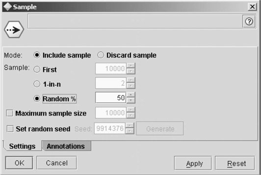
Figure 8-2 This dialog box illustrates the random assignment of data into training and test samples. (Screenshot taken by the author is from Clementine 8.5.)
Another consideration is when and how frequently to conduct the random assignment to the groups. In a perfect world, it would not matter. The sample could be split each and every time the model is adjusted, modified, and tested because the samples would be similar each time and the model would be robust enough to accommodate any slight differences. In fact, this is how some random assignment software procedures function. In reality, however, it can happen that the samples are comparable, the model development is progressing nicely, and on the next iteration something happens, the training sample differs significantly from the test sample, and everything falls apart. When this occurs, the analyst might be perplexed and goes back and refines the model in an effort to accommodate this new development, but on the next iteration nothing works again. This can go on almost indefinitely. Because of this possibility, it is generally best to split the sample, ensure that they are comparable, particularly on the dimensions of interest, and then move forward into model development and testing with a confidence that the training and test samples are similar, yet randomly divided.
In modeling a particularly low-frequency event, it is important to ensure that the factors of potential interest are distributed evenly. Because they are assigned randomly to the training and test samples, it is possible that the analyst could end up with an uneven distribution that would skew the model based on certain features or attributes that are associated with a few, unique cases. For example, Table 8-1 depicts a small sample of ages that were entered randomly into a database. The data shown is confined to the portion of the sample of interest, or the cases that we would like to model and predict. A quick check reveals that the average age of the entire list of cases is 31 years; however, the average age of the training sample is 24 years, while the average age of the test sample is 39 years. Is this a problem? It depends. If age was included as a discriminating or predictive variable in the model because of these artificial differences in the averages then, yes, this nonrandom selection could have a significant impact on the created model. It could be that age makes no difference, that the comparison sample, which has not been shown here, also has an average age of 31 years. The uneven selection of the training sample, however, generated an average age of 24 years, which might be different enough to be included as a predictive factor in the model. When we come back with the test sample, however, the average age is 39 years. With differences like these, it is relatively easy to see how the performance of the model might suffer when tested with a sample that differs so significantly on a relevant variable. Similarly, if an average age of 24 was included in the model as a predictive variable, it would perform very poorly when deployed in an operational setting. This highlights further the importance of using training and test samples during the development process. Therefore, running a few quick comparisons between the training and test samples on variables of interest can be helpful in ensuring that they are as similar as possible and ultimately in protecting the outcomes.
Table 8-1 A small sample of age data that has been divided into training and test samples. It is important to ensure that training and test samples are similar, particularly when they are relatively small.
| Age | Sample |
| 25 | Train |
| 45 | Test |
| 24 | Train |
| 38 | Test |
| 23 | Train |
| 32 | Test |
| 21 | Train |
| 45 | Test |
| 24 | Train |
| 35 | Test |
| 27 | Train |
| 39 | Test |
| 24 | Train |
| 37 | Test |
Remember that it also is important to consider the distribution of the outcome of interest between the training and test samples. For example, if the model being created is to predict which robberies are likely to escalate into aggravated assaults, there might be hundreds of robberies available for the generation of the model but only a small fraction that actually escalated into an aggravated assault. In an effort to ensure that the model has access to a sufficient number of cases and that the created model accurately predicts the same or a very similar ratio of incidents, it is important to ensure that these low-frequency events are adequately represented in the modeling process. When working with very small numbers, training and test sample differences of even a few cases can really skew the outcomes, both in terms of predictive factors and predicted probabilities.
Sometimes, the events of interest are so rare that splitting them into training and test samples reduces the number to the point where it seriously compromises the ability to generate a valid model. Techniques such as boosting, which increases the representation of low-frequency events in the sample, can be used, but they should be employed and interpreted cautiously, as they also increase the likelihood that unusual or unique attributes will be magnified. It is important to monitor the prior probabilities when boosting is used to ensure that the predicted probabilities reflect the prior, not boosted, probabilities. In addition, other methods of testing the model should be considered, such as bootstrapping, in which each case is tested individually against a model generated using the remainder of the sample. These techniques are beyond the scope of this text, but interested readers can refer to their particular software support for additional information and guidance.
8.4 Evaluating the Model
While overall accuracy would appear to be the best method for evaluating a model, it tends to be somewhat limited in the applied public safety and security setting given the relative infrequency of the events studied. As mentioned previously, it is possible to attain a high, overall level of accuracy in a model created to predict infrequent events by predicting that they would never happen. Moreover, it is often the case that the behavior of interest is not only infrequent but also heterogeneous, because criminals tend to commit crime in slightly different, individual ways. Increasing the fidelity of the models in an effort to overcome the rarity of these events and accurately discriminating the cases or incidents of interest may include accurate measurement and use of the expected or prior probabilities and subtle adjustment of the costs to shift the nature and distribution of errors into an acceptable range. Prior probabilities are used in the modeling process to ensure that the models constructed reflect the relative probability of incidents or cases observed during training, while adjusting the costs can shift the distribution and nature of the errors to better match the overall requirements of the analytical task. The following section details the use of confusion matrices in the evaluation of model accuracy, as well as the nature and distribution of errors.
Confusion matrices were introduced in Chapter 1. A confusion matrix can help determine the specific nature of errors when testing a model. While the overall accuracy of the model has value, it generally should be used only as an initial screening tool. A final decision regarding whether the model is actionable should be postponed until it can be evaluated in light of the specific distribution and nature of the errors within the context of its ultimate use. Under the harsh light of this type of thoughtful review, many “perfect” models have been discarded in favor of additional analysis because the nature of the errors was unacceptable.
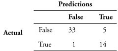
Table 8-2 provides an example of a typical confusion matrix. In this example, a total of 53 cases were classified with 47 of them, or almost 89%, being classified correctly. The overall accuracy of this model is good, but it is important to determine the exact nature of the errors. By drilling down and reviewing the specific errors, we see that 33 of 38 “false” predictions, or 87%, were classified correctly. Further review indicates that 14 of 15 “true” predictions, or 93%, also were classified correctly. In public safety and intelligence modeling, these results would be extremely impressive, so much so that additional review probably would be required to ensure that there were no errors in logic that could have contributed to such an accurate model.
The confusion matrix for a second model with the same sample is depicted in Table 8-3. The overall accuracy of this model is much lower, 70%, but there has been no degradation in the accuracy of predicting “true” events, which is still 93%. Most of the errors with this model occur when the model incorrectly predicts that something will happen. In other words, most of the decrease in overall accuracy of the model is associated with false positives.
Table 8-3 The overall accuracy of this model is much lower than that seen in Table 8-2, but there has been no degradation in the accuracy of predicting “true” events. Most of the decrease in overall accuracy of this model is associated with false positives.

Clearly, if we had to choose between the two models, the first model with its greater overall accuracy would be the obvious choice. What happens, however, if we are developing a deployment model and the first model is too complicated to be actionable? Can we use the second model with any confidence? It is important to think through the consequences to determine whether this model will suffice.
The second model accurately predicts that something will occur 93% of the time. As a deployment model, this means that by using this model we are likely to have an officer present when needed 93% of the time, which is excellent. As compared to many traditional methods of deployment, which include historical precedence, gut feelings, and citizen demands for increased police presence, this model almost certainly represents a significant increase over chance that our officers will be deployed when and where they are likely to be needed.
Conversely, most of the errors in this model are associated with false positives, which means that the model predicts deployment for a particular time or place where 39% of the time nothing will occur. From a resource management standpoint, this means that those resources were deployed when they were not needed and were wasted. But were they? When dealing with public safety, it is almost always better to err on the side of caution. Moreover, in all reality, it is highly unlikely that the officers deployed to locations or times that were not associated with an increased risk wasted their time. Opportunities for increased citizen contact and self-initiated patrol activities abound. Therefore, although the model was overly generous in terms of resource deployment, it performed better than traditional methods. Thoughtful consideration of the results still supports the use of a model with this pattern of accuracy and errors for deployment.
In the next confusion matrix (Table 8-4), we see an overall classification accuracy of 78%. While this is not bad for a model that will be used in policing, a potential problem occurs when we examine the “true” predictions. In this example, the “true” classifications are accurate only about 50% of the time. In other words, we could attain the same level of accuracy by flipping a coin; the model performs no better than chance in predicting true occurrences. If this performance is so low, then why is the overall level of accuracy relatively high, particularly in comparison? Like many examples in law enforcement and intelligence analysis, we are trying to predict relatively low-frequency events. Because they are so infrequent, the diminished accuracy associated with predicting these events contributes less to the overall accuracy of the model.
Table 8-4 The overall classification accuracy of this model is not terrible; however, the “true” classifications are accurate only about 50% of the time. This poor performance does not significantly degrade the overall accuracy because it is associated with a low-frequency event.

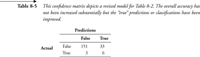
As can be seen in the confusion matrix in Table 8-5, which is associated with a revised model for the previous example, the overall accuracy has not been increased substantially, but the “true” predictions or classifications have been improved to an accuracy of 67%. Additional thought will be required to determine whether this level of accuracy is acceptable. For deployment purposes, almost anything above chance has the potential to increase public safety; however, it must be determined whether failing to place resources one-third of the time when they are likely to be needed is acceptable. On the other hand, if this model was associated with automated motive determination or some sort of relatively inconsequential anomaly detection, then the comparatively low false positive rate might be of some benefit. A good understanding of the limitations of this model in determining actual events is imperative to ensuring that it is used properly.
Table 8-5 This confidence matrix depicts a revised model for Table 8-2. The overall accuracy has not been increased substantially but the “true” predictions or classifications have been improved.
8.5 Updating or Refreshing the Model
In our experience, models need to be refreshed on a relatively regular basis. In some ways, this is a measure of success. Many features, particularly behavioral characteristics, are unique to particular offenders. As these suspects are identified and apprehended, new criminals take their places, and the patterns and trends change. In most situations, the changes are minimal, although they still frequently warrant a revised model.
Seasonal changes can have an effect on some patterns of offending. As mentioned, during the colder months, people often heat their vehicles in the mornings before they leave the house. Therefore, lower temperatures would be associated with an increased prevalence of vehicles stolen from residential areas, with an increased frequency in the mornings when both the weather and vehicles are colder. When temperatures climb, people often leave their vehicles running while they make quick stops, in an effort to keep their cars cool. A model tracking these incidents might predict an increase in motor vehicle thefts near convenience stores and day care centers, possibly later in the day, when temperatures are higher. Therefore, a motor vehicle theft model that takes into account these trends might need to be refreshed or rotated seasonally. It also might require a greater sampling frame, or time span of data, to ensure that all of the trends and patterns have been captured.
8.6 Caveat Emptor
There is one area in which to be particularly cautious when using some outside consultants. As mentioned earlier, it is relatively easy to develop a model that describes existing data very well but that is over-trained and therefore relatively inaccurate with new data. In other words, the model has been refined to the point where it describes all of the little flaws and idiosyncrasies associated with that particular sample. It is highly predictive of the training data, but when checked against an independent sample of test data, the flaws are revealed through compromised accuracy. Unfortunately when this happens, the outside “expert” generally is gone, and the locals left behind might mistakenly assume the blame for the poor outcome. This can be particularly troubling in situations where accurately evaluating the performance of the model is beyond the technical expertise of the customer. In this situation, the same consultant is rehired and then “fixes” the model, generally by overfitting it to a new set of sample data.
The best way to evaluate the performance of a model is to see how well it can predict or classify a second sample, whether a “test” sample or future data. Be particularly leery of any consultant who advises you that he or she will “adjust” the model until it reaches a certain level of performance, which frequently is very high, but warns you that in your hands the accuracy of the model is likely to decrease significantly. Generally, what these folks are doing is “overfitting” the model to increase the apparent accuracy. The performance of these models often will decrease significantly when used on new data, and frequently will perform far worse than a more general, less accurate model. At a minimum, the informed consumer will require that any outside consultant employ both training and test samples to ensure a minimal level of stability in the performance of the model. An even better scenario results when the agency analyzes its own data and creates its own models, perhaps with some outside assistance or analytical support and guidance. It is the folks on the inside that have the best understanding of where the data came from and how the model will be used. These individuals also have the requisite domain expertise, or knowledge of crime and criminals, that is necessary to generate meaningful data mining solutions. Generally, for law enforcement personnel to use predictive analytics effectively, some guidance is required regarding a few “rules of the road” and best practices, like the use of training and test samples, and perhaps some analytical support. But in my experience, this is not an overwhelming challenge.
Finally, it is important to remember that the cost of errors in the applied public safety setting frequently is life itself. Therefore, specific attention to errors and the nature of errors is required. In some situations, anything that brings decision accuracy above chance is adequate. In other situations, however, errors in analysis or interpretation can result in misallocated resources, wasted time, and even loss of life.