The method used in the layer-wise training of DBN, pre-training, is called Restricted Boltzmann Machines (RBM). To begin with, let's take a look at the RBM that forms the basis of DBN. As RBM stands for Restricted Boltzmann Machines, of course there's a method called Boltzmann Machines (BMs). Or rather, BMs are a more standard form and RBM is the special case of them. Both are one of the neural networks and both were proposed by Professor Hinton.

The implementation of RBM and DBNs can be done without understanding the detailed theory of BMs, but in order to understand these concepts, we'll briefly look at the idea BMs are based on. First of all, let's look at the following figure, which shows a graphical model of BMs:

BMs look intricate because they are fully connected, but they are actually just simple neural networks with two layers. By rearranging all the units in the networks to get a better understanding, BMs can be shown as follows:

Please bear in mind that normally the input/output layer is called the visible layer in BMs and RBMs (a hidden layer is commonly used as it is), for it is the networks that presume the hidden condition (unobservable condition) from the observable condition. Also, the neurons of the visible layer are called visible units and the neurons of the hidden layer are called hidden units. Signs in the previous figure are described to match the given names.

As you can see in the diagram, the structure of BMs is not that different from standard neural networks. However, its way of thinking has a big feature. The feature is to adopt the concept of energy in neural networks. Each unit has a stochastic state respectively and the whole of the networks' energy is determined depending on what state each unit takes. (The first model that adopted the concept of energy in networks is called the Hopfield network, and BMs are the developed version of it. Since details of the Hopfield network are not totally relevant to deep learning, it is not explained in this book.) The condition that memorizes the correct data is the steady state of networks and the least amount of energy these networks have. On the other hand, if data with noise is provided to the network, each unit has a different state, but not a steady state, hence its condition makes the transition to stabilize the whole network, in other words, to transform it into a steady state.

This means that the weights of the model are adjusted and the state of each unit is transferred to minimize the energy function the networks have. These operations can remove the noise and extract the feature from inputs as a whole. Although the energy of networks sounds enormous, it's not too difficult to imagine because minimizing the energy function has the same effect as minimizing the error function.

The concept of BMs was wonderful, but various problems occurred when BMs were actually applied to practical problems. The biggest problem was that BMs are fully connected networks and take an enormous amount of calculation time. Therefore, RBM was devised. RBM is the algorithm that can solve various problems in a realistic time frame by making BMs restricted. Just as in BM, RBM is a model based on the energy of a network. Let's look at RBM in the diagram below:

Here, is the number of units in the visible layer and the number of units in the hidden layer. denotes the value of a visible unit, the value of a hidden unit, and the weight between these two units. As you can see, the difference between BM and RBM is that RBM doesn't have connections between the same layer. Because of this restriction, the amount of calculation decreases and it can be applied to realistic problems.

Now, let's look through the theory.

If we expand the theory, it can also handle continuous values. However, this could make equations complex, where it's not the core of the theory and where it's implemented with binary in the original DBN proposed by Professor Hinton. Therefore, we'll also implement binary RBM in this book. RBM with binary inputs is sometimes called Bernoulli RBM.

RBM is the energy-based model, and the status of a visible layer or hidden layer is treated as a stochastic variable. We'll look at the equations in order. First of all, each visible unit is propagated to the hidden units throughout a network. At this time, each hidden unit takes a binary value based on the probability distribution generated in accordance with its propagated inputs:

Here, is the bias in a hidden layer and denotes the sigmoid function.

This time, it was conversely propagated from a hidden layer to a visible layer through the same network. As in the previous case, each visible unit takes a binary value based on probability distribution generated in accordance with propagated values.

Here, is the bias of the visible layer. This value of visible units is expected to match the original input values. This means if , the weight of the network as a model parameter, and , , the bias of a visible layer and a hidden layer, are shown as a vector parameter, , it leans in order for the probability that can be obtained above to get close to the distribution of .

For this learning, the energy function, that is, the evaluation function, needs to be defined. The energy function is shown as follows:

Also, the joint probability density function showing the demeanor of a network can be shown as follows:

From the preceding formulas, the equations for the training of parameters will be determined. We can get the following equation:

Hence, the log likelihood can be shown as follows:

Then, we'll calculate each gradient against the model parameter. The derivative can be calculated as follows:

Some equations in the middle are complicated, but it turns out to be simple with the term of the probability distribution of the model and the original data.

Therefore, the gradient of each parameter is shown as follows:

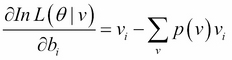
Now then, we could find the equation of the gradient, but a problem occurs when we try to apply this equation as it is. Think about the term of . This term implies that we have to calculate the probability distribution for all the {0, 1} patterns, which can be assumed as input data that includes patterns that don't actually exist in the data.

We can easily imagine how this term can cause a combinatorial explosion, meaning we can't solve it within a realistic time frame. To solve this problem, the method for approximating data using Gibbs sampling, called Contrastive Divergence (CD), was introduced. Let's look at this method now.

Here, is an input vector. Also, is an input (output) vector that can be obtained by sampling for k-times using this input vector.

Then, we get:

Hence, when approximating after reiterating Gibbs sampling, the derivative of the log likelihood function can be represented as follows:

Therefore, the model parameter can be shown as follows:

Here, is the number of iterations and is the learning rate. As shown in the preceding formulas, generally, CD that performs sampling k-times is shown as CD-k. It's known that CD-1 is sufficient when applying the algorithm to realistic problems.

Now, let's go through the implementation of RMB. The package structure is as shown in the following screenshot:

Let's look through the RestrictedBoltzmannMachines.java file. Because the first part of the main method just defines the variables needed for a model and generates demo data, we won't look at it here.

So, in the part where we generate an instance of a model, you may notice there are many null values in arguments:

// construct RBM
RestrictedBoltzmannMachines nn = new RestrictedBoltzmannMachines(nVisible, nHidden, null, null, null, rng);

When you look at the constructor, you might know that these null values are the RBM's weight matrix, bias of hidden units, and bias of visible units. We define arguments as null here because they are for DBN's implementation. In the constructor, these are initialized as follows:

   if (W == null) {

       W = new double[nHidden][nVisible];
       double w_ = 1. / nVisible;

       for (int j = 0; j < nHidden; j++) {
           for (int i = 0; i < nVisible; i++) {
               W[j][i] = uniform(-w_, w_, rng);
           }
       }
   }

   if (hbias == null) {
       hbias = new double[nHidden];

       for (int j = 0; j < nHidden; j++) {
           hbias[j] = 0.;
       }
   }

   if (vbias == null) {
       vbias = new double[nVisible];

       for (int i = 0; i < nVisible; i++) {
           vbias[i] = 0.;
       }
   }

The next step is training. CD-1 is applied for each mini-batch:

// train with contrastive divergence
for (int epoch = 0; epoch < epochs; epoch++) {
   for (int batch = 0; batch < minibatch_N; batch++) {
       nn.contrastiveDivergence(train_X_minibatch[batch], minibatchSize, learningRate, 1);
   }
   learningRate *= 0.995;
}

Now, let's look into the essential point of RBM, the contrastiveDivergence method. CD-1 can obtain a sufficient solution when we actually run this program (and so we have k = 1 in the demo), but this method is defined to deal with CD-k as well:

// CD-k : CD-1 is enough for sampling (i.e. k = 1)
sampleHgivenV(X[n], phMean_, phSample_);

for (int step = 0; step < k; step++) {

   // Gibbs sampling
   if (step == 0) {
       gibbsHVH(phSample_, nvMeans_, nvSamples_, nhMeans_, nhSamples_);
   } else {
       gibbsHVH(nhSamples_, nvMeans_, nvSamples_, nhMeans_, nhSamples_);
   }

}

It appears that two different types of method, sampleHgivenV and gibbsHVH, are used in CD-k, but when you look into gibbsHVH, you can see:

public void gibbsHVH(int[] h0Sample, double[] nvMeans, int[] nvSamples, double[] nhMeans, int[] nhSamples) {
   sampleVgivenH(h0Sample, nvMeans, nvSamples);
   sampleHgivenV(nvSamples, nhMeans, nhSamples);
}

So, CD-k consists of only two methods for sampling, sampleVgivenH and sampleHgivenV.

As the name of the method indicates, sampleHgivenV is the method that sets the probability distribution and sampling data generated in a hidden layer based on the given value of visible units and vice versa:

public void sampleHgivenV(int[] v0Sample, double[] mean, int[] sample) {

   for (int j = 0; j < nHidden; j++) {
       mean[j] = propup(v0Sample, W[j], hbias[j]);
       sample[j] = binomial(1, mean[j], rng);
   }

}

public void sampleVgivenH(int[] h0Sample, double[] mean, int[] sample) {

   for(int i = 0; i < nVisible; i++) {
       mean[i] = propdown(h0Sample, i, vbias[i]);
       sample[i] = binomial(1, mean[i], rng);
   }
}

The propup and propdown tags that set values to respective means are the method that activates values of each unit by the sigmoid function:

public double propup(int[] v, double[] w, double bias) {

   double preActivation = 0.;

   for (int i = 0; i < nVisible; i++) {
       preActivation += w[i] * v[i];
   }
   preActivation += bias;

   return sigmoid(preActivation);
}

public double propdown(int[] h, int i, double bias) {

   double preActivation = 0.;

   for (int j = 0; j < nHidden; j++) {
       preActivation += W[j][i] * h[j];
   }
   preActivation += bias;

   return sigmoid(preActivation);
}

The binomial method that sets a value to a sample is defined in RandomGenerator.java. The method returns 0 or 1 based on the binomial distribution. With this method, a value of each unit becomes binary:

public static int binomial(int n, double p, Random rng) {
   if(p < 0 || p > 1) return 0;

   int c = 0;
   double r;

   for(int i=0; i<n; i++) {
       r = rng.nextDouble();
       if (r < p) c++;
   }

   return c;
}

Once approximated values are obtained by sampling, what we need to do is just calculate the gradient of a model parameter and renew a parameter using a mini-batch. There's nothing special here:

// calculate gradients
for (int j = 0; j < nHidden; j++) {
   for (int i = 0; i < nVisible; i++) {
       grad_W[j][i] += phMean_[j] * X[n][i] - nhMeans_[j] * nvSamples_[i];
   }

   grad_hbias[j] += phMean_[j] - nhMeans_[j];
}

for (int i = 0; i < nVisible; i++) {
   grad_vbias[i] += X[n][i] - nvSamples_[i];
}


// update params
for (int j = 0; j < nHidden; j++) {
   for (int i = 0; i < nVisible; i++) {
       W[j][i] += learningRate * grad_W[j][i] / minibatchSize;
   }

   hbias[j] += learningRate * grad_hbias[j] / minibatchSize;
}

for (int i = 0; i < nVisible; i++) {
   vbias[i] += learningRate * grad_vbias[i] / minibatchSize;
}

Now we're done with the model training. Next comes the test and evaluation in general cases, but note that the model cannot be evaluated with barometers such as accuracy because RBM is a generative model. Instead, let's briefly look at how noisy data is changed by RBM here. Since RBM after training can be seen as a neural network, the weights of which are adjusted, the model can obtain reconstructed data by simply propagating input data (that is, noisy data) through a network:

public double[] reconstruct(int[] v) {

   double[] x = new double[nVisible];
   double[] h = new double[nHidden];

   for (int j = 0; j < nHidden; j++) {
       h[j] = propup(v, W[j], hbias[j]);
   }

   for (int i = 0; i < nVisible; i++) {
       double preActivation_ = 0.;

       for (int j = 0; j < nHidden; j++) {
           preActivation_ += W[j][i] * h[j];
       }
       preActivation_ += vbias[i];

       x[i] = sigmoid(preActivation_);
   }

   return x;
}

DBNs are deep neural networks where logistic regression is added to RBMS as the output layer. Since the theory necessary for implementation has already been explained, we can go directly to the implementation. The package structure is as follows:

The flow of the program is very simple. The order is as follows:

Just as in RBM, the first step in setting up the main method is the declaration of variables and the code for creating demo data (the explanation is omitted here).

Please check that in the demo data, the number of units for an input layer is 60, a hidden layer has 2 layers, their combined number of units is 20, and the number of units for an output layer is 3. Now, let's look through the code from the Building the Model section:

// construct DBN
System.out.print("Building the model...");
DeepBeliefNets classifier = new DeepBeliefNets(nIn, hiddenLayerSizes, nOut, rng);
Sy
stem.out.println("done.");

The variable of hiddenLayerSizes is an array and its length represents the number of hidden layers in deep neural networks. The deep learning algorithm takes a huge amount of calculation, hence the program gives us an output of the current status so that we can see which process is proceeding. The variable of hiddenLayerSizes is an array and its length represents the number of hidden layers in deep neural networks. Each layer is constructed in the constructor.

This is because, as explained in the theory section, pre-training performs layer-wise training, whereas the whole model can be regarded as one neural network:

// construct multi-layer
for (int i = 0; i < nLayers; i++) {
   int nIn_;
   if (i == 0) nIn_ = nIn;
   else nIn_ = hiddenLayerSizes[i-1];

   // construct hidden layers with sigmoid function
   //   weight matrices and bias vectors will be shared with RBM layers
   sigmoidLayers[i] = new HiddenLayer(nIn_, hiddenLayerSizes[i], null, null, rng, "sigmoid");

   // construct RBM layers
   rbmLayers[i] = new RestrictedBoltzmannMachines(nIn_, hiddenLayerSizes[i], sigmoidLayers[i].W, sigmoidLayers[i].b, null, rng);
}

// logistic regression layer for output
logisticLayer = new LogisticRegression(hiddenLayerSizes[nLayers-1], nOut);

The first thing to do after building the model is pre-training:

// pre-training the model
System.out.print("Pre-training the model...");
classifier.pretrain(train_X_minibatch, minibatchSize, train_minibatch_N, pretrainEpochs, pretrainLearningRate, k);
System.out.println("done.");

Pre-training needs to be processed with each minibatch but, at the same time, with each layer. Therefore, all training data is given to the pretrain method first, and then the data of each mini-batch is processed in the method:

public void pretrain(int[][][] X, int minibatchSize, int minibatch_N, int epochs, double learningRate, int k) {

   for (int layer = 0; layer < nLayers; layer++) {  // pre-train layer-wise
       for (int epoch = 0; epoch < epochs; epoch++) {
           for (int batch = 0; batch < minibatch_N; batch++) {

               int[][] X_ = new int[minibatchSize][nIn];
               int[][] prevLayerX_;

               // Set input data for current layer
               if (layer == 0) {
                   X_ = X[batch];
               } else {

                   prevLayerX_ = X_;
                   X_ = new int[minibatchSize][hiddenLayerSizes[layer-1]];

                   for (int i = 0; i < minibatchSize; i++) {
                       X_[i] = sigmoidLayers[layer-1].outputBinomial(prevLayerX_[i], rng);
                   }
               }

               rbmLayers[layer].contrastiveDivergence(X_, minibatchSize, learningRate, k);
           }
       }
   }

}

Since the actual learning is done through CD-1 of RBM, the description of DBN within the code is very simple. In DBN (RBM), units of each layer have binary values, so the output method of HiddenLayer cannot be used because it returns double. Hence, the outputBinomial method is added to the class, which returns the int type (the code is omitted here). Once the pre-training is complete, the next step is fine-tuning.

We can easily fall into overfitting if we use the whole data set for both pre-training and fine-tuning. Therefore, the validation data set is prepared separately from the training dataset and is used for fine-tuning:

// fine-tuning the model
System.out.print("Fine-tuning the model...");
for (int epoch = 0; epoch < finetuneEpochs; epoch++) {
   for (int batch = 0; batch < validation_minibatch_N; batch++) {
       classifier.finetune(validation_X_minibatch[batch], validation_T_minibatch[batch], minibatchSize, finetuneLearningRate);
   }
   finetuneLearningRate *= 0.98;
}
System.out.println("done.");

In the finetune method, the backpropagation algorithm in multi-layer neural networks is applied where the logistic regression is used for the output layer. To backpropagate unit values among multiple hidden layers, we define variables to maintain each layer's inputs:

public void finetune(double[][] X, int[][] T, int minibatchSize, double learningRate) {

   List<double[][]> layerInputs = new ArrayList<>(nLayers + 1);
   layerInputs.add(X);

   double[][] Z = new double[0][0];
   double[][] dY;

   // forward hidden layers
   for (int layer = 0; layer < nLayers; layer++) {

       double[] x_;  // layer input
       double[][] Z_ = new double[minibatchSize][hiddenLayerSizes[layer]];

       for (int n = 0; n < minibatchSize; n++) {

           if (layer == 0) {
               x_ = X[n];
           } else {
               x_ = Z[n];
           }

           Z_[n] = sigmoidLayers[layer].forward(x_);
       }

       Z = Z_.clone();
       layerInputs.add(Z.clone());
   }

   // forward & backward output layer
   dY = logisticLayer.train(Z, T, minibatchSize, learningRate);

   // backward hidden layers
   double[][] Wprev;
   double[][] dZ = new double[0][0];

   for (int layer = nLayers - 1; layer >= 0; layer--) {

       if (layer == nLayers - 1) {
           Wprev = logisticLayer.W;
       } else {
           Wprev = sigmoidLayers[layer+1].W;
           dY = dZ.clone();
       }

       dZ = sigmoidLayers[layer].backward(layerInputs.get(layer), layerInputs.get(layer+1), dY, Wprev, minibatchSize, learningRate);
   }
}

The training part of DBN is just how it is seen in the preceding code. The hard part is probably the theory and implementation of RBM, so you might think it's not too hard when you just look at the code of DBN.

Since DBN after the training can be regarded as one (deep) neural network, you simply need to forward propagate data in each layer when you try to predict which class the unknown data belongs to:

public Integer[] predict(double[] x) {

   double[] z = new double[0];

   for (int layer = 0; layer < nLayers; layer++) {

       double[] x_;

       if (layer == 0) {
           x_ = x;
       } else {
           x_ = z.clone();
       }

       z = sigmoidLayers[layer].forward(x_);
   }

   return logisticLayer.predict(z);
}

As for evaluation, no explanation should be needed because it's not much different from the previous classifier model.

Congratulations! You have now acquired knowledge of one of the deep learning algorithms. You might be able to understand it more easily than expected. However, the difficult part of deep learning is actually setting up the parameters, such as setting how many hidden layers there are, how many units there are in each hidden layer, the learning rate, the iteration numbers, and so on. There are way more parameters to set than in the method of machine learning. Please remember that you might find this point difficult when you apply this to a realistic problem.

The method used in pre-training for SDA is called Denoising Autoencoders (DA). It can be said that DA is the method that emphasizes the role of equating inputs and outputs. What does this mean? The processing content of DA is as follows: DA adds some noise to input data intentionally and partially damages the data, and then DA performs learning as it restores corrupted data to the original input data. This intentional noise can be easily substantiated if the input data value is [0, 1]; by turning the value of the relevant part into 0 compulsorily. If a data value is out of this range, it can be realized, for example, by adding Gaussian noise, but in this book, we'll think about the former [0, 1] case to understand the core part of the algorithm.

In DA as well, an input/output layer is called a visible layer. DA's graphical model can be shown to be the same shape of RBM, but to get a better understanding, let's follow this diagram:

Here, is the corrupted data, the input data with noise. Then, forward propagation to the hidden layer and the output layer can be represented as follows:

Here, denotes the bias of the hidden layer and the bias of the visible layer. Also, denotes the sigmoid function. As seen in the preceding diagram, corrupting input data and mapping to a hidden layer is called Encode and mapping to restore the encoded data to the original input data is called Decode. Then, DA's evaluation function can be denoted with a negative log likelihood function of the original input data and decoded data:

Here, is the model parameter, the weight and the bias of the visible layer and the hidden layer. What we need to do is just find the gradients of these parameters against the evaluation function. To deform equations easily, we define the functions here:

Then, we get:

Using these functions, each gradient of a parameter can be shown as follows:

Therefore, only two terms are required. Let's derive them one by one:

Here, we utilized the derivative of the sigmoid function:

Also, we get:

Therefore, the following equation can be obtained:

On the other hand, we can also get the following:

Hence, the renewed equation for each parameter will be as follows:

Here, is the number of iterations and is the learning rate. Although DA requires a bit of technique for deformation, you can see that the theory itself is very simple compared to RBM.

Now, let's proceed with the implementation. The package structure is the same as the one for RBM.

As for model parameters, in addition to the number of units in a hidden layer, the amount of noise being added to the input data is also a parameter in DA. Here, the corruption level is set at 0.3. Generally, this value is often set at 0.1 ~ 0.3:

double corruptionLevel = 0.3;

The flow from the building model to training is the same as RBM. Although this method of training is called contrastiveDivergence in RBM, it's simply set as train in DA:

// construct DA
DenoisingAutoencoders nn = new DenoisingAutoencoders(nVisible, nHidden, null, null, null, rng);

// train
for (int epoch = 0; epoch < epochs; epoch++) {
   for (int batch = 0; batch < minibatch_N; batch++) {
       nn.train(train_X_minibatch[batch], minibatchSize, learningRate, corruptionLevel);
   }
}

The content of train is as explained in the theory section. First of all, add noise to the input data, then encode and decode it:

// add noise to original inputs
double[] corruptedInput = getCorruptedInput(X[n], corruptionLevel);

// encode
double[] z = getHiddenValues(corruptedInput);

// decode
double[] y = getReconstructedInput(z);

The process of adding noise is, as previously explained, the compulsory turning of the value of the corresponding part of the data into 0:

public double[] getCorruptedInput(double[] x, double corruptionLevel) {

   double[] corruptedInput = new double[x.length];

   // add masking noise
   for (int i = 0; i < x.length; i++) {
       double rand_ = rng.nextDouble();

       if (rand_ < corruptionLevel) {
           corruptedInput[i] = 0.;
       } else {
           corruptedInput[i] = x[i];
       }
   }

   return corruptedInput;
}

The other processes are just simple activation and propagation, so we won't go through them here. The calculation of the gradients follows math equations:

// calculate gradients

// vbias
double[] v_ = new double[nVisible];

for (int i = 0; i < nVisible; i++) {
   v_[i] = X[n][i] - y[i];
   grad_vbias[i] += v_[i];
}

// hbias
double[] h_ = new double[nHidden];

for (int j = 0; j < nHidden; j++) {

   for (int i = 0; i < nVisible; i++) {
       h_[j] = W[j][i] * (X[n][i] - y[i]);
   }

   h_[j] *= z[j] * (1 - z[j]);
   grad_hbias[j] += h_[j];
}

// W
for (int j = 0; j < nHidden; j++) {
   for (int i = 0; i < nVisible; i++) {
       grad_W[j][i] += h_[j] * corruptedInput[i] + v_[i] * z[j];
   }
}

Compared to RBM, the implementation of DA is also quite simple. When you test (reconstruct) the model, you don't need to corrupt the data. As in standard neural networks, you just need to forward propagate the given inputs based on the weights of the networks:

public double[] reconstruct(double[] x) {

   double[] z = getHiddenValues(x);
   double[] y = getReconstructedInput(z);

   return y;
}

SDA is deep neural networks with piled up DA layers. In the same way that DBN consists of RBMs and logistic regression, SDA consists of DAs and logistic regression:

The flow of implementation is not that different between DBN and SDA. Even though there is a difference between RBM and DA in pre-training, the content of fine-tuning is exactly the same. Therefore, not much explanation might be needed.

The method for pre-training is not that different, but please note that the point where the int type was used for DBN is changed to double type, as DA can handle [0, 1], not binary:

public void pretrain(double[][][] X, int minibatchSize, int minibatch_N, int epochs, double learningRate, double corruptionLevel) {

   for (int layer = 0; layer < nLayers; layer++) {
       for (int epoch = 0; epoch < epochs; epoch++) {
           for (int batch = 0; batch < minibatch_N; batch++) {

               double[][] X_ = new double[minibatchSize][nIn];
               double[][] prevLayerX_;

               // Set input data for current layer
               if (layer == 0) {
                   X_ = X[batch];
               } else {

                 prevLayerX_ = X_;
                 X_ = new double[minibatchSize][hiddenLayerSizes[layer-1]];

                   for (int i = 0; i < minibatchSize; i++) {
                       X_[i] = sigmoidLayers[layer-1].output(prevLayerX_[i]);
                   }
               }

               daLayers[layer].train(X_, minibatchSize, learningRate, corruptionLevel);
           }
       }
   }

}

The predict method after learning is also exactly the same as in DBN. Considering that both DBN and SDA can be treated as one multi-layer neural network after learning (that is, the pre-training and fine-tuning), it's natural that most of the processes are common.

Overall, SDA can be implemented more easily than DBN, but the precision to be obtained is almost the same. This is the merit of SDA.